Working Group 3 - Chapter 3: Issues related to mitigation in the long-term context - (AR4-WG3-3)
Original at: http://www.ipcc.ch/publications_and_data/ar4/wg3/en/ch3.html
Main AR4 Index | Working Group WG3 Index | Table of Contents | Authors | Executive Summary | Annotated Text | References | Reviewer Comments
With the exception of Chapter and Section headings, all coloured text has been inserted by AccessIPCC. The non-coloured text is the IPCC original.
A number of emails from the Climate Research Unit (CRU) of the University of East Anglia were published on the Internet in November 2009. This has provided a window into the world of climate science.
We have identified a number of key individuals involved in the emails whom we have designated as Persons of Concern [PoC]; a Journal in which a PoC has published has been designated as a Journal of Concern [JoC].
This is not to suggest that we believe such papers are necessarily flawed, but rather that, as Joseph Alcamo noted at Bali in October 2009, "as policymakers and the public begin to grasp the multi-billion dollar price tag for mitigating and adapting to climate change, we should expect a sharper questioning of the science behind climate policy".
References occur in a list at the end of each chapter. Citations are within the normal text of sections and paragraphs.
| Tag | Explanation | Where Used | References | Citations |
|---|---|---|---|---|
| PoC |
Person of Concern Key individual involved in CRU emails as defined in this spreadsheet. |
References, Citations, IPCC Roles | 11 | 14 |
| JoC |
Journal of Concern A Journal which has published articles by one or more PoCs (Person of Concern) |
References, Citations | 69 | 107 |
| MoS |
Model or Simulation Reference appears to be a model or simulation, not observation or experiment |
References, Citations | 85 | 142 |
| NPR |
Non Peer Reviewed Reference has no Journal or no Volume or no Pages or it has Editors. |
References, Citations | 175 | 339 |
| SRC |
Self Reference Concern Author of a chapter containing references to own work. |
References, Citations, IPCC Roles | 83 | 241 |
| ARC |
Paper authored or co-authored by person who is also in list of Authors of another chapter. |
References, Citations | 46 | 71 |
| 2007 |
Paper dated 2007, when IPCC policy stated cutoff was December 2005 |
References, Citations | 9 | 60 |
| Ambiguous |
The short inline citation matched with more than one reference; however, AccessIPCC will link to the first reference found. |
Citations | - | 8 |
| NotFound |
The short inline citation was not matched with any reference. Believed to be caused by typing errors. |
Citations | - | 3 |
| Clean |
The reference was probably peer reviewed. |
References, Citations | 52 | 54 |
Coordinating Lead Authors:
Brian Fisher (Australia) [SRC:5], Nebojsa Nakicenovic (Austria/Montenegro) [SRC:11],
| Concern | Occurrence |
|---|---|
| SRC >= 5 | 2 |
| Potentially Biased Authors | 2 |
Lead Authors:
Knut Alfsen (Norway) [SRC:3], Jan Corfee Morlot (France/USA), Francisco de la Chesnaye (USA) [SRC:4], Jean-Charles Hourcade (France) [SRC:1], Kejun Jiang (China) [SRC:3], Mikiko Kainuma (Japan) [SRC:4], Emilio La Rovere (Brazil) [SRC:5], Anna Matysek (Australia) [SRC:1], Ashish Rana (India) [SRC:2], Keywan Riahi (Austria) [SRC:14], Richard Richels (USA) [SRC:6], Steven Rose (USA) [SRC:1], Detlef Van Vuuren (The Netherlands) [SRC:19], Rachel Warren (UK) [SRC:1],
| Concern | Occurrence |
|---|---|
| SRC >= 5 | 4 |
| SRC 1-4 | 9 |
| Potentially Biased Authors | 13 |
| Impartial Authors | 1 |
Contributing Authors:
Phillipe Ambrosi (France) [SRC:2], Fatih Birol (Turkey), Daniel Bouille (Argentina), Christa Clapp (USA), Bas Eickhout (The Netherlands) [SRC:8], Tatsuya Hanaoka (Japan) [SRC:2], Michael D. Mastrandrea (USA) [SRC:3], Yuzuru Matsuoko (Japan), Brian O’Neill (USA) [SRC:7], Hugh Pitcher (USA) [SRC:6], Shilpa Rao (India) [SRC:3], Ferenc Toth (Hungary) [SRC:4],
| Concern | Occurrence |
|---|---|
| SRC >= 5 | 3 |
| SRC 1-4 | 5 |
| Potentially Biased Authors | 8 |
| Impartial Authors | 4 |
Review Editors:
John Weyant (USA) [SRC:5], Mustafa Babiker (Kuwait) [SRC:3],
| Concern | Occurrence |
|---|---|
| SRC >= 5 | 1 |
| SRC 1-4 | 1 |
| Potentially Biased Authors | 2 |
This chapter should be cited as:
Fisher, B.S., N. Nakicenovic, K. Alfsen, J. Corfee Morlot, F. de la Chesnaye, J.-Ch. Hourcade, K. Jiang, M. Kainuma, E. La Rovere, A. Matysek, A. Rana, K. Riahi, R. Richels, S. Rose, D. van Vuuren, R. Warren, 2007: Issues related to mitigation in the long term context, In Climate Change 2007: Mitigation. Contribution of Working Group III to the Fourth Assessment Report of the Inter-governmental Panel on Climate Change [B. Metz, O.R. Davidson, P.R. Bosch, R. Dave, L.A. Meyer (eds)], Cambridge University Press, Cambridge, United Kingdom and New York, NY, USA.
EXECUTIVE SUMMARY
This chapter documents baseline and stabilization scenarios in the literature since the publication of the IPCC Special Report on Emissions Scenarios SRES ( Nakicenovic et al., 2000 [NPR, SRC] ) and Third Assessment Report (TAR, Morita et al., 2001 [NPR, SRC] ). It reviews the use of the SRES reference and TAR stabilization scenarios and compares them with new scenarios that have been developed during the past five years. Of special relevance is how ranges published for driving forces and emissions in the newer literature compare with those used in the TAR, SRES and pre-SRES scenarios. This chapter focuses particularly on the scenarios that stabilize atmospheric concentrations of greenhouse gases (GHGs). The multi-gas stabilization scenarios represent a significant change in the new literature compared to the TAR, which focused mostly on carbon dioxide (CO2) emissions. They also explore lower levels and a wider range of stabilization than in the TAR.
The foremost finding from the comparison of the SRES and new scenarios in the literature is that the ranges of main driving forces and emissions have not changed very much (high agreement, much evidence). Overall, the emission ranges from scenarios without climate policy reported before and after the SRES have not changed appreciably. Some changes are noted for population and economic growth assumptions. Population scenarios from major demographic institutions are lower than they were at the time of the SRES, but so far they have not been fully implemented in the emissions scenarios in the literature. All other factors being equal, lower population projections are likely to result in lower emissions. However, in the scenarios that used lower projections, changes in other drivers of emissions have offset their impact. Regional medium-term ( 2030 ) economic projections for some developing country regions are currently lower than the highest scenarios used in the SRES. Otherwise, economic growth perspectives have not changed much, even though they are among the most intensely debated aspects of the SRES scenarios. In terms of emissions, the most noticeable changes occurred for projections of SOx and NOx emissions. As short-term trends have moved down, the range of projections for both is currently lower than the range published before the SRES. A small number of new scenarios have begun to explore emission pathways for black and organic carbon.
Baseline land-related CO2 and non-CO2 GHG emissions remain significant, with continued but slowing land conversion and increased use of high-emitting agricultural intensification practices due to rising global food demand and shifts in dietary preferences towards meat consumption. The post-SRES scenarios suggest a degree of agreement that the decline in annual land-use change carbon emissions will, over time, be less dramatic (slower) than those suggested by many of the SRES scenarios. Global long-term land-use scenarios are scarce in numbers but growing, with the majority of the new literature since the SRES contributing new forestry and biomass scenarios. However, the explicit modelling of land-use in long-term global scenarios is still relatively immature, with significant opportunities for improvement.
In the debate on the use of exchange rates, market exchange rates (MER) or purchasing power parities (PPP), evidence from the limited number of new PPP-based studies indicates that the choice of metric for gross domestic product (GDP), MER or PPP, does not appreciably affect the projected emissions, when metrics are used consistently. The differences, if any, are small compared to the uncertainties caused by assumptions on other parameters, e.g. technological change (high agreement, much evidence).
The numerical expression of GDP clearly depends on conversion measures; thus GDP expressed in PPP will deviate from GDP expressed in MER, more so for developing countries. The choice of conversion factor (MER or PPP) depends on the type of analysis or comparison being undertaken. However, when it comes to calculating emissions (or other physical measures, such as energy), the choice between MER-based or PPP-based representations of GDP should not matter, since emission intensities will change (in a compensating manner) when the GDP numbers change. Thus, if a consistent set of metrics is employed, the choice of MER or PPP should not appreciably affect the final emission levels (high agreement, medium evidence). This supports the SRES in the sense that the use of MER or PPP does not, in itself, lead to significantly different emission projections outside the range of the literature (high agreement, much evidence). In the case of the SRES, the emissions trajectories were the same whether economic activities in the four scenario families were measured in MER or PPP.
Some studies find differences in emission levels between using PPP-based and MER-based estimates. These results critically depend on, among other things, convergence assumptions (high agreement, medium evidence). In some of the short-term scenarios (with a horizon to 2030 ) a ‘bottom-up’ approach is taken, where assumptions about productivity growth and investment and saving decisions are the main drivers of growth in the models. In long-term scenario models, a ‘top-down’ approach is more commonly used, where the actual growth rates are more directly prescribed based on convergence or other assumptions about long-term growth potentials. Different results can also be due to inconsistencies in adjusting the metrics of energy efficiency improvement when moving from MER-based to PPP-based calculations.
There is a clear and strong correlation between the CO2-equivalent concentrations (or radiative forcing) of the published studies and the CO2-only concentrations by 2100, because CO2 is the most important contributor to radiative forcing. Based on this relationship, to facilitate scenario comparison and assessment, stabilization scenarios (both multi-gas and CO2-only studies) have been grouped in this chapter into different categories that vary in the stringency of the targets, from low to high radiative forcing, CO2-equivalent concentrations and CO2-only concentrations by 2100, respectively.
Essentially, any specific concentration or radiative forcing target, from the lowest to the highest, requires emissions to eventually fall to very low levels as the removal processes of the ocean and terrestrial systems saturate. For low to medium targets, this would need to occur during this century, but higher stabilization targets can push back the timing of such reductions to beyond 2100 . However, to reach a given stabilization target, emissions must ultimately be reduced well below current levels. For achievement of the very low stabilization targets from many high baseline scenarios, negative net emissions are required towards the end of the century. Mitigation efforts over the next two or three decades will have a large impact on opportunities to achieve lower stabilization levels (high agreement, much evidence).
The timing of emission reductions depends on the stringency of the stabilization target. Lowest stabilization targets require an earlier peak of CO2 and CO2-equivalent emissions. In the majority of the scenarios in the most stringent stabilization category (a stabilization level below 490 ppmv CO2-equivalent), emissions are required to decline before 2015 and are further reduced to less than 50% of today’s emissions by 2050 . For somewhat higher stabilization levels (e.g. below 590 ppmv CO2-equivalent) global emissions in the scenarios generally peak around 2010 – 2030, followed by a return to 2000 levels, on average around 2040 . For high stabilization levels (e.g. below 710 ppmv CO2-equivalent) the median emissions peak around 2040 (high agreement, much evidence).
Long-term stabilization scenarios highlight the importance of technology improvements, advanced technologies, learning-by-doing, and induced technological change, both for achieving the stabilization targets and cost reduction (high agreement, much evidence). While the technology improvement and use of advanced technologies have been employed in scenarios largely exogenously in most of the literature, new literature covers learning-by-doing and endogenous technological change. The latter scenarios show different technology dynamics and ways in which technologies are deployed, while maintaining the key role of technology in achieving stabilization and cost reduction.
Decarbonization trends are persistent in the majority of intervention and non-intervention scenarios (high agreement, much evidence). The medians of scenario sets indicate decarbonization rates of around 0.9 (pre-TAR) and 0.6 (post-TAR) compared to historical rates of about 0.3% per year. Improvements of carbon intensity of energy supply and the whole economic need to be much faster than in the past for the low stabilization levels. On the upper end of the range, decarbonization rates of up to 2.5% per year are observed in more stringent stabilization scenarios, where complete transition away from carbon-intensive fuels is considered.
The scenarios that report quantitative results with drastic CO2 reduction targets of 60–80% in 2050 (compared to today’s emission levels) require increased rates of energy intensity and carbon intensity improvement by 2–3 times their historical levels. This is found to require different sets of mitigation options across regions, with varying shares of nuclear energy, carbon capture and storage (CCS), hydrogen, and biomass.
The costs of stabilization crucially depend on the choice of the baseline, related technological change and resulting baseline emissions; stabilization target and level; and the portfolio of technologies considered (high agreement, much evidence). Additional factors include assumptions with regard to the use of flexible instruments and with respect to revenue recycling. Some literature identifies low-cost technology clusters that allow for endogenous technological learning with uncertainty. This suggests that a decarbonized economy may not cost any more than a carbon-intensive one, if technological learning is taken into account.
There are different metrics for reporting costs of emission reductions, although most models report them in macro-economic indicators, particularly GDP losses. For stabilization at 4–5 W/m2 (or ~ 590–710 ppmv CO2-equivalent) macro-economic costs range from -1 to 2% of GDP below baseline in 2050 . For a more stringent target of 3.5–4.0 W/m2 (~ 535–590 ppmv CO2-equivalent) the costs range from slightly negative to 4% GDP loss (high agreement, much evidence). GDP losses in the lowest stabilization scenarios in the literature (445-535 ppmv CO2-equivalent) are generally below 5.5% by 2050, however the number of studies are relatively limited and are developed from predominantly low baselines (high agreement, medium evidence).
Multi-gas emission-reduction scenarios are able to meet climate targets at substantially lower costs compared to CO2-only strategies (for the same targets, high agreement, much evidence). Inclusion of non-CO2 gases provides a more diversified approach that offers greater flexibility in the timing of the reduction programme.
Including land-use mitigation options as abatement strategies provides greater flexibility and cost-effectiveness for achieving stabilization (high agreement, medium evidence). Even if land activities are not considered as mitigation alternatives by policy, consideration of land (land-use and land cover) is crucial in climate stabilization for its significant atmospheric inputs and withdrawals (emissions, sequestration, and albedo). Recent stabilization studies indicate that land-use mitigation options could provide 15–40% of total cumulative abatement over the century. Agriculture and forestry mitigation options are projected to be cost-effective abatement strategies across the entire century. In some scenarios, increased commercial biomass energy (solid and liquid fuel) is a significant abatement strategy, providing 5–30% of cumulative abatement and potentially 1–15% of total primary energy over the century.
Decision-making concerning the appropriate level of mitigation in a cost-benefit context is an iterative risk-management process that considers investment in mitigation and adaptation, co-benefits of undertaking climate change decisions and the damages due to climate change. It is intertwined with development decisions and pathways. Cost-benefit analysis tries to quantify climate change damages in monetary terms as the social cost of carbon (SCC) or time-discounted damages. Due to considerable uncertainties and difficulties in quantifying non-market damages, it is difficult to estimate SCC with confidence. Results depend on a large number of normative and empirical assumptions that are not known with any certainty. SCC estimates in the literature vary by three orders of magnitude. Often they are likely to be understated and will increase a few percent per year (i.e. 2.4% for carbon-only and 2–4% for the social costs of other greenhouse gases ( IPCC, 2007b [NPR, 2007] , Chapter 20). SCC estimates for 2030 range between 8 and 189 US$/tCO2-equivalent ( IPCC, 2007b [NPR, 2007] , Chapter 20), which compares to carbon prices between 1 to 24 US$/tCO2-equivalent for mitigations scenarios stabilizing between 485-570 ppmv CO2-equivalent) and 31 to 121 US$/tCO2-equivalent for scenarios stabilizing between 440-485 ppmv CO2-equivalent, respectively (high agreement, limited evidence).
For any given stabilization pathway, a higher climate sensitivity raises the probability of exceeding temperature thresholds for key vulnerabilities (high agreement, much evidence). For example, policymakers may want to use the highest values of climate sensitivity (i.e. 4.5°C) within the ‘likely’ range of 2–4.5°C set out by IPCC 2007a [NPR, 2007] , Chapter 10) to guide decisions, which would mean that achieving a target of 2°C (above the pre-industrial level), at equilibrium, is already outside the range of scenarios considered in this chapter, whilst a target of 3°C (above the pre-industrial level) would imply stringent mitigation scenarios, with emissions peaking within 10 years. Using the ‘best estimate’ assumption of climate sensitivity, the most stringent scenarios (stabilizing at 445–490 ppmv CO2-equivalent) could limit global mean temperature increases to 2–2.4°C above the pre-industrial level, at equilibrium, requiring emissions to peak before 2015 and to be around 50% of current levels by 2050 . Scenarios stabilizing at 535–590 ppmv CO2-equivalent could limit the increase to 2.8–3.2°C above the pre-industrial level and those at 590–710 CO2-equivalent to 3.2–4°C, requiring emissions to peak within the next 25 and 55 years, respectively (high agreement, medium evidence).
Decisions to delay emission reductions seriously constrain opportunities to achieve low stabilization targets (e.g. stabilizing concentrations from 445–535 ppmv CO2-equivalent), and raise the risk of progressively more severe climate change impacts and key vulnerabilities occurring.
The risk of climate feedbacks is generally not included in the above analysis. Feedbacks between the carbon cycle and climate change affect the required mitigation for a particular stabilization level of atmospheric CO2 concentration. These feedbacks are expected to increase the fraction of anthropogenic emissions that remains in the atmosphere as the climate system warms. Therefore, the emission reductions to meet a particular stabilization level reported in the mitigation studies assessed here might be underestimated.
Short-term mitigation and adaptation decisions are related to long-term climate goals (high agreement, much evidence). A risk management or ‘hedging’ approach can assist policymakers to advance mitigation decisions in the absence of a long-term target and in the face of considerable uncertainties relating to the cost of mitigation, the efficacy of adaptation and the negative impacts of climate change. The extent and the timing of the desirable hedging strategy will depend on the stakes, the odds and societies’ attitudes to risks, for example with respect to risks of abrupt change in geo-physical systems and other key vulnerabilities. A variety of integrated assessment approaches exist to assess mitigation benefits in the context of policy decisions relating to such long-term climate goals. There will be ample opportunity for learning and mid-course corrections as new information becomes available. However, actions in the short term will largely determine what future climate change impacts can be avoided. Hence, analysis of short-term decisions should not be decoupled from analysis that considers long-term climate change outcomes (high agreement, much evidence).
3.1 Emissions scenarios
The evolution of future greenhouse gas emissions and their underlying driving forces is highly uncertain, as reflected in the wide range of future emissions pathways across (more than 750) emission scenarios in the literature. This chapter assesses this literature, focusing especially on new multi-gas baseline scenarios produced since the publication of the IPCC Special Report on Emissions Scenarios SRES ( Nakicenovic et al., 2000 [NPR, SRC] ) and on new multi-gas mitigation scenarios in the literature since the publication of the IPCC Third Assessment Report (TAR, Working Group III, Chapter 2 Morita et al., 2001 [NPR, SRC] ). This literature is referred to as ‘post-SRES’ scenarios.
The SRES scenarios were representative of some 500 emissions scenarios in the literature, grouped as A1, A2, B1 and B2, at the time of their publication in 2000 . Of special relevance in this review is the question of how representative the SRES ranges of driving forces and emission levels are of the newer scenarios in the literature, and how representative the TAR stabilization levels and mitigation options are compared with the new multi-gas stabilization scenarios. Other important aspects of this review include methodological, data and other advances since the time the SRES scenarios were developed.
This chapter uses the results of the Energy Modeling Forum (EMF-21) scenarios and the new Innovation Modelling Comparison Project (IMCP) network scenarios. In contrast to SRES and post-SRES scenarios, these new modelling-comparison activities are not based on fully harmonized baseline scenario assumptions, but rather on ‘modeller’s choice’ scenarios. Thus, further uncertainties have been introduced due to different assumptions and different modelling approaches. Another emerging complication is that even baseline (also called reference) scenarios include some explicit policies directed at emissions reduction, notably due to the Kyoto Protocol entering into force, and other climate-related policies that are being implemented in many parts of the world.
Another difficulty in straightforward comparisons is that the information and documentation of the scenarios in the literature varies considerably.
3.1.1 The definition and purpose of scenarios
Scenarios describe possible future developments. They can be used in an exploratory manner or for a scientific assessment in order to understand the functioning of an investigated system ( Carpenter et al., 2005 [NPR] ).
In the context of the IPCC assessments, scenarios are directed at exploring possible future emissions pathways, their main underlying driving forces and how these might be affected by policy interventions. The IPCC evaluation of emissions scenarios in 1994 identified four main purposes of emissions scenarios ( Alcamo et al., 1995 [NPR, MoS, ARC] ):
- To provide input for evaluating climatic and environmental consequences of alternative future GHG emissions in the absence of specific measures to reduce such emissions or enhance GHG sinks.
- To provide similar input for cases with specific alternative policy interventions to reduce GHG emissions and enhance sinks.
- To provide input for assessing mitigation and adaptation possibilities, and their costs, in different regions and economic sectors.
- To provide input to negotiations of possible agreements to reduce GHG emissions.
Scenario definitions in the literature differ depending on the purpose of the scenarios and how they were developed. The SRES report ( Nakicenovic et al., 2000 [NPR, SRC] ) defines a scenario as a plausible description of how the future might develop, based on a coherent and internally consistent set of assumptions (‘scenario logic’) about the key relationships and driving forces (e.g. rate of technology change or prices). Some studies in the literature apply the term ‘scenario’ to ‘best-guess’ or forecast types of projections. Such studies do not aim primarily at exploring alternative futures, but rather at identifying ‘most likely’ outcomes. Probabilistic studies represent a different approach, in which the range of outcomes is based on a consistent estimate of the probability density function (PDF) for crucial input parameters. In these cases, outcomes are associated with an explicit estimate of likelihood, albeit one with a substantial subjective component. Examples include probabilistic projections for population ( Lutz and Sanderson, 2001 [JoC] ) and CO2 emissions ( Webster et al., 2002 [MoS, SRC] , 2003; O’Neill, 2004 [NPR, MoS, SRC] ).
3.1.1.1 Types of scenarios
The scenario literature can be split into two largely non-overlapping streams – quantitative modelling and qualitative narratives ( Morita et al., 2001 [NPR, SRC] ). This dualism mirrors the twin challenges of providing systematic and replicable quantitative representation, on the one hand, and contrasting social visions and non-quantifiable descriptors, on the other ( Raskin et al., 2005 [NPR, SRC] ). It is particularly noteworthy that recent developments in scenario analysis are beginning to bridge this difficult gap ( Nakicenovic et al., 2000 [NPR, SRC] ; Morita et al., 2001 [NPR, SRC] ; and Carpenter et al., 2005 ).
Catastrophic futures feature prominently in the narrative scenarios literature. They typically involve large-scale environmental or economic collapse, extrapolating current unfavourable conditions and trends in many regions. [1] Many of these scenarios suggest that catastrophic developments may draw the world into a state of chaos within one or two decades. Greenhouse-gas emissions might be low in such scenarios because of low or negative economic growth, but seem unlikely to receive much attention in any case, in the light of more immediate problems. This report does not analyze such futures, except where cases provide emissions pathways.
3.1.1.2 Narrative storylines and modelling
The literature based on narrative storylines that describe futures is rich going back to the first global studies of the 1970 s (e.g. Kahn et al., 1976 [NPR] ; Kahn and Weiner, 1967 [NPR] ) and is also well represented in more recent literature (e.g. ( Peterson and Peterson, 1994; ) Gallopin et al., 1997 [NPR, ARC] ; Raskin et al., 1998 [NPR, ARC] ; Glenn and Gordon, 1997 [NPR, MoS] ). Well known are the Shell scenarios that are principally based on narrative stories with illustrative quantification of salient driving forces and scenario outcomes ( (Wack, 1985a, ) 1985b; Schwartz, 1991 [NPR] ; Shell, 2005 ).
3.1.1.3 Global futures scenarios
Global futures scenarios are deeply rooted in the long history of narrative scenarios ( Carpenter et al., 2005 [NPR] ; UNEP, 2002 [NPR, MoS] ). The direct antecedents of contemporary scenarios lie with the future studies of the 1970 s ( Raskin et al., 2005 [NPR, SRC] ). These responded to emerging concerns about the long-term sufficiency of natural resources to support expanding global populations and economies. This first wave of global scenarios included ambitious mathematical simulation models ( Meadows et al., 1972 [NPR] ; Mesarovic and Pestel, 1974 [NPR] ) as well as speculative narrative ( Kahn et al., 1976 [NPR] ). At this time, scenario analysis was first used at Royal Dutch/Shell as a strategic management technique ( (Wack, 1985a, ) 1985b; Schwartz, 1991 [NPR] ).
A second round of integrated global analysis began in the late 1980 s and 1990 s, prompted by concerns with climate change and sustainable development. These included narratives of alternative futures ranging from ‘optimistic’ and ‘pessimistic’ worlds to consideration of ‘surprising’ futures ( Burrows et al., 1991 [NPR, MoS] ; the Central Planning Bureau of the Netherlands, 1992; ( Kaplan, 1994; ) Svedin and Aniansson, 1987 [NPR, MoS] ; Toth et al., 1989 [NPR, SRC] ). The long-term nature of the climate change issue introduced a new dimension and has resulted in a rich new literature of global emissions scenarios, starting from the IPCC IS92 scenarios ( Pepper et al., 1992 [NPR, ARC] ; Leggett et al., 1992 [NPR, ARC] ) and most recent scenario comparisons projects (e.g. EMF and IMCP). The first decades of scenario assessment paved the way by showing the power – and limits – of both deterministic modelling and descriptive future analyses. A central challenge of global scenario exercises today is to unify these two aspects by blending the objectivity and clarity of quantification with the richness of narrative ( Raskin et al., 2005 [NPR, SRC] ).
3.1.2 Introduction to mitigation and stabilization scenarios
Climate change intervention, control, or mitigation scenarios capture measures and policies for reducing GHG emissions with respect to some baseline (or reference) scenario. They contain emission profiles, as well as costs associated with the emissions reduction, but often do not quantify the benefits of reduced impacts from climate change. Stabilization scenarios are mitigation scenarios that aim at a pre-specified GHG reduction pathway, leading to stabilization of GHG concentrations in the atmosphere.
For the purposes of this chapter, a scenario is identified as a mitigation or intervention scenario if it meets one of the following two conditions:
- It incorporates specific climate change targets, which may include absolute or relative GHG limits, GHG concentration levels (e.g. CO2 or CO2-equivalent (CO2-eq) stabilization scenarios), or maximum allowable changes in temperature or sea level.
- It includes explicit or implicit policies and/or measures of which the primary goal is to reduce CO2 or a broader range of GHG emissions (e.g. a carbon tax, carbon cap or a policy encouraging the use of renewable energy).
Some scenarios in the literature are difficult to classify as mitigation (intervention) or baseline (reference or non-intervention), such as those developed to assess sustainable development (SD) paths. These studies consider futures that require radical policy and behavioural changes to achieve a transition to a postulated sustainable development pathway. Greenpeace formulated one of the first such scenarios ( Lazarus et al., 1993 [NPR, MoS] ). Many sustainable development scenarios are also included in this assessment. Where they do not include explicit policies, as in the case of SRES scenarios, they can be classified as baseline or non-intervention scenarios. For example, the SRES B1 family of reference scenarios can be characterized as having many elements of a sustainability transition that lead to generally low GHG emissions, even though the scenarios do not include policies or measures explicitly directed at emissions mitigation.
Another type of mitigation (intervention or climate policy) scenario approach specifies future ‘worlds’ that are internally consistent with some specified climate target (e.g. a global temperature increase of no more than 1°C by 2100 ), and then works backwards to develop feasible emission trajectories and emission driver combinations leading to these targets. Such scenarios, also referred to as ‘safe landing’ or ‘tolerable window’ scenarios, imply the necessary development and implementation of climate policies intended to achieve these targets in the most efficient way ( Morita et al., 2001 [NPR, SRC] ). A number of such new multi-gas stabilization scenarios are assessed in this chapter.
Confusion can arise when the inclusion of ‘non-climate-related’ policies in a reference (non-intervention) scenario has the effect of significantly reducing GHG emissions. For example, energy efficiency or land-use policies that reduce GHG emissions may be adopted for reasons that are not related to climate policies and may therefore be included in a non-intervention scenario. Such a scenario may include GHG emissions that are lower than some intervention scenarios. The root cause of this potential confusion is that, in practice, many policies can both reduce GHG emissions and achieve other goals (so-called multiple benefits). Whether such policies are assumed to be adopted for climate or non-climate policy-related reasons is determined by the scenario developer, based on the underlying scenario narrative. While this is a problem in terms of making a clear distinction between intervention and non-intervention scenarios, it is at the same time an opportunity. Because many decisions are not made for reasons of climate change alone, measures implemented for reasons other than climate change can have a significant impact on GHG emissions, opening up many new possibilities for mitigation ( Morita et al., 2001 [NPR, SRC] ).
3.1.3 Development trends and the lock-in effect of infrastructure choices
An important consideration in scenario generation is the nature of the economic development process and whether (and to what extent) developing countries will follow the development pathways of industrialized countries with respect to energy use and GHG emissions. The ‘lock-in’ effects of infrastructure, technology and product design choices made by industrialized countries in the post-World War II period of low energy prices are responsible for the major recent increase in world GHG emissions. A simple mimicking by developing countries of the development paradigm established by industrialized countries could lead to a very large increase in global GHG emissions (see Chapter 2 ). It may be noted, however, that energy/GDP elasticities in industrialized countries have first increased in successive stages of industrialization, with acceleration during the 1950 s and 1960 s, but have fallen sharply since then, due to factors such as relative growth of services in GDP share, technical progress induced by higher oil prices and energy conservation efforts.
In developing countries, where a major part of the infrastructure necessary to meet development needs is still to be built, the spectrum of future options is considerably wider than in industrialized countries (e.g. on energy, see IEA, 2004 [NPR] ). The spatial distribution of the population and economic activities is still not settled, opening the possibility of adopting industrial policies directed towards rural development and integrated urban, regional, and transportation planning, thereby avoiding urban sprawl and facilitating more efficient transportation and energy systems. The main issue is the magnitude and viability to tap the potential for technological ‘leapfrogging’, whereby developing countries can bypass emissions-intensive intermediate technology and jump straight to cleaner technologies. There are technical possibilities for less energy-intensive development patterns in the long run, leading to low carbon futures in southern countries that are compatible with national objectives (see e.g. la Rovere and Americano, 2002 [JoC, SRC] ). Section 12.2 of Chapter 12 develops this argument further.
On the other hand, the barriers to such development pathways should not be underestimated, going from financial constraints to cultural behaviours in industrialized and developing countries, including the lack of appropriate institution building. One of the key findings of the reviewed literature is the long-term implications for GHG emissions of short- and medium-term decisions concerning the building of new infrastructure, particularly in developing countries (see e.g. la Rovere and Americano, 2002 [JoC, SRC] ; IEA, 2004 [NPR] ).
3.1.4 Economic growth and convergence
Determinants of long-term GDP per person include labour force and its productivity projections. Labour force utilization depends on factors such as the number of working-age people, the level of structural unemployment and hours worked per worker. Demographic change is still the major determinant of the baseline labour supply ( Martins and Nicoletti, 2005 [NPR, MoS] ). Long-term projections of labour productivity primarily depend on improvements in labour quality (capacity building) and the pace of technical change associated with building up the capital-output ratio and the quality of capital.
The literature examining production functions shows increasing returns because of an expanding stock of human capital and, as a result of specialization and investment in ‘knowledge’ capital ( Meier, 2001 [NPR, MoS] ; Aghion and Howitt, 1998 [NPR] ), suggests that economic ‘catch-up’ and convergence strongly depend on the forces of ‘technological congruence’ and ‘social capability’ between the productivity leader and the followers (see the subsequent sub-section on institutional frameworks and Section 3.4 on the role of technological change).
The economic convergence literature ( (Abramovitz, 1986; ) ( Baumol, 1986 ) ), using a standard neoclassical economic growth setup following ( Solow 1956 ) ), found evidence of convergence only between the richest countries. Other research efforts documented ‘conditional convergence’ – meaning that countries appeared to reach their own steady states at a fairly uniform rate of 2% per year ( (Barro, 1991; ) ( Mankiw et al., 1992 ) ( Jones 1997 ) ) found that the future steady-state distribution of per person income will be broadly similar to the 1990 distribution. Important differences would continue to arise among the bottom two-thirds of the income distribution, thus confirming past trends. Total factor productivity (TFP) levels and convergence for the evolution of income distribution are also important. Expected catch-up, and even overtaking per-person incomes, as well as changes in leaders in the world distribution of income, are among some of the findings in this literature. ( Quah 1993, ) 1996 ) found that the world is moving towards a bimodal income distribution. Some recent assessments demonstrate divergence, not convergence (World Bank, 2002 [NPR] ; Halloy and Lockwood, 2005 [NPR] ; UNSD, 2005 [NPR] ).
Convergence is limited for a number of reasons, such as imperfect mobility of factors (notably labour); different endowments (notably human capital); market segmentation (notably services); and limited technology diffusion. Social inertia (as referred to in Chapter 2 , see Section 2.2.3 ) also contributes to delay convergence. Therefore only limited catch-up can be factored in baseline scenarios: while capital quality is likely to push up productivity growth in most countries, especially in those lagging behind, labour quality is likely to drag down productivity growth in a number of countries, unless there are massive investments in education. However, appropriate policies may accelerate the adoption of new technologies and create incentives for human capital formation and thus accelerate convergence ( Martins and Nicoletti, 2005 [NPR, MoS] ). Nelson and Fagerberg, arguing within an evolutionary paradigm, have different perspectives on the convergence issue ( (Fagerberg, 1995; ) Fagerberg and Godinho, 2005 [NPR] ; UNIDO, 2005 [NPR] ). It should be acknowledged that the old theoretical controversy about steady-state economics and limits to growth still continues (Georgescu-Roegen, 1971 ).
The above discussion provides the economic background for the range of assumptions on the long-term convergence of income between developing and developed countries (measured by GDP per person) found in the scenario literature. The annual rate of income convergence between 11 world regions in the SRES scenarios falls within the range of less than 0.5% in the A2 scenario family to less than 2% in A1 (both in PPP and MER metrics). The highest rate of income convergence in the SRES is similar to the observed convergence, during the period 1950 – 1990, of 90 regions in Europe ( (Barro and Sala-i-Martin 1997 ) ). However, Grübler et al. 2006 [NPR, SRC] ) note that extending convergence analysis to national or sub-national level would suggest that income disparities are larger than suggested by simple inter-regional comparisons and that scenarios of (relative) income convergence are highly sensitive to the spatial level of aggregation used in the analysis. An important finding from the sensitivity analysis performed is that less convergence generally yields higher emissions ( Grübler et al., 2004 [SRC] ). In B2, an income ratio (between 11 world regions, in market exchange rates) of seven corresponds to CO2 emissions of 14.2 GtC in 2100, while shifting this income ratio to 16 would lead to CO2 emissions of 15.5 GtC in 2100 . Results pointing in the same direction were also obtained for A2. This can be explained by slower TFP growth, slower capital turnover, and less ‘technological congruence’, leading to slower adoption of low-emission technologies in developing countries. On the other hand, as climate stabilization scenarios require global application of climate policies and convergence in the adoption of low-emission technologies, they are less compatible with low economic convergence scenarios.
3.1.5 Development pathways and GHG emissions
In the long run, the links between economic development and GHG emissions depend not only on the growth rate (measured in aggregate terms), but also on the nature and structure of this growth. Comparative studies aiming to explain these differences help to determine the main factors that will ultimately influence the amount of GHG emissions, given an assumed overall rate of economic growth ( Jung et al., 2000 [SRC] ; see also examples discussed in Section 12.2 of Chapter 12 ).
- Structural changes in the production system, namely the role of high or low energy-intensive industries and services.
- Technological patterns in sectors such as energy, transportation, building, waste, agriculture and forestry – the treatment of technology in economic models has received considerable attention and triggered the most difficult debates within the scientific community working in this field (Edmonds and Clarke, 2005; Grubb et al., 2005; Shukla, 2005; Worrell, 2005; Köhler et al., 2006).
- Geographical distribution of activities encompassing both human settlements and urban structures in a given territory, and its twofold impact on the evolution of land use, and on mobility needs and transportation requirements.
- Consumption patterns – existing differences between countries are mainly due to inequalities in income distribution, but for a given income per person, parameters such as housing patterns, leisure styles, or the durability and rate of obsolescence of consumption goods will have a critical influence on long-run emission profiles.
- Trade patterns – the degree of protectionism and the creation of regional blocks can influence access to the best available technologies, inter alia, and constraints on financial flows can limit the capacity of developing countries to build their infrastructure.
These different relationships between development pathways and GHG emissions may (or may not) be captured in models used for long-term world scenarios, by changes in aggregated variables (e.g. per person income) or through more disaggregated economic parameters, such as the structure of expenses devoted to a given need (e.g. heating, transport or food, or the share of energy and transportation in the production function of industrial sectors). This means that alternative configurations of these underlying factors can be combined to give internally consistent socio-economic scenarios with identical rates of economic growth. It would be false to say that current economic models ignore these factors. They are to some extent captured by changes in economic parameters, such as the structure of household expenses devoted to heating, transportation or food; the share of each activity in the total household budget; and the share of energy and transportation costs in total costs in the industrial sector.
These parameters remain important, but the outcome in terms of GHG emissions will also depend on dynamic links between technology, consumption patterns, transportation and urban infrastructure, urban planning, and rural-urban distribution of the population (see also Chapters 2 and 11 for more extensive discussions of some of these issues).
3.1.6 Institutional frameworks
Recent research has included studies on the role of institutions as a critical component in an economy’s capacity to use resources optimally ( Ostrom, 1990 [NPR] ; Ostrom et al., 2002 [NPR] ) and interventions that alter institutional structure are among the most accepted solutions in recent times for shaping economic structure and its associated energy use and emissions. Three important aspects of institutional structure are:
1. The extent of centralization and participation in decisions.
2. The extent (spanning from local to global) and nature of decision mechanisms.
3. Processes for effective interventions (e.g. the mix of market and regulatory processes).
Institutional structures vary considerably across nations, even those with similar levels of economic development. Although no consensus exists on the desirability of a specific type of institutional framework, experience suggests that more participative processes help to build trust and social capital to better manage the environmental ‘commons’ (World Bank, 1992 [NPR] ; Beierle and Cayford, 2002 [NPR, MoS] ; Ostrom et al., 2002 [NPR] ; Rydin, 2003 [NPR] ). Other relevant developments may include greater use of market mechanisms and institutions to enhance global cooperation and more effectively manage global environmental issues (see also Chapter 12 ).
A weak institutional structure basically explains why an economy can be in a position that is significantly below the theoretically efficient production frontier, with several economists terming it as a ‘missing link’ in the production function ( Meier, 2001 [NPR, MoS] ). Furthermore, weak institutions also cause frictions in economic exchange processes, resulting in high transaction costs.
The existence of weak institutions in developing countries has implications for the capacity to adapt to or mitigate climate change. A review of the social capital literature and the implications for climate change mitigation policies concludes that successful implementation of GHG emission-reduction options will generally depend on additional measures to increase the potential market and the number of exchanges. This can involve strengthening the incentives for exchange (prices, capital markets, information efforts, etc.), introducing new actors (institutional and human capacity efforts), and reducing the risks of participating (legal framework, information, general policy context of market regulation). The measures all depend on the nature of the formal institutions, the social groups in society, and the interaction between them (see Chapter 2 and Halsnaes, 2002 [NPR, ARC] ).
Some of the climate change policy recommendations that are inspired by institutional economics include general capacity-building programmes, and local enterprise and finance development, for example in the form of soft loans, in addition to educational and training programmes ( Halsnaes, 2002 [NPR, ARC] , see also Chapters 2 and 12 ).
In today’s less industrialized regions, there is a large and relatively unskilled part of the population that is not yet involved in the formal economy. In many regions industrialization leads to wage differentials that draw these people into the more productive, formal economy, causing accelerated urbanization in the process. This is why labour force growth in these regions contributes significantly to GDP growth. The concerns relating to the informal economy are twofold:
1. Whether historical development patterns and relationships among key underlying variables will hold constant in the projections period.
2. Whether there are important feedbacks between the evolution of a particular sector and the overall development pattern that would affect GHG emissions ( Shukla, 2005 [NPR, ARC] ).
Social and cultural processes shape institutions and the way in which they function. Social norms of ownership and distribution have a vital influence on the structure of production and consumption, as well as the quality and extent of the social ‘infrastructure’ sectors, such as education, which are paramount to capacity building and technological progress. Unlike institutions, social and culture processes are often more inflexible and difficult to influence. However, specific sectors, such as education, are amenable to interventions. Barring some negative features, such as segregation, there is no consensus as to the interventions that are necessary or desirable to alter social and cultural processes. On the other hand, understanding their role is crucial for assessing the evolution of the social infrastructure that underpins technological progress and human welfare ( Jung et al., 2000 [SRC] ) as well as evolving perceptions and social understanding of climate change risk (see Rayner and Malone, 1998 [NPR, ARC] ; Douglas and Wildavsky, 1982 [NPR] ; Slovic, 2000 [NPR] ).
While institutional arrangements are sometimes described as part of storylines, scenario specifications generally do not include explicit assumptions about them. The role of institutions in the implementation of development choices and its implications to climate change mitigation are discussed further in Section 12.2 of Chapter 12 .
3.2 Baseline scenarios
3.2.1 Drivers of emissions
Trajectories of future emissions are determined by complex dynamic processes that are influenced by factors such as demographic and socio-economic development, as well as technological and institutional change. An often-used identity to describe changes in some of these factors is based on the IPAT identity (Impact = Population x Affluence x Technology – see ( Holdren, 2000; ) Ehrlich and Holdren, 1971 [JoC] ) and in emissions modelling is often called the ‘Kaya identity’ (see Section 3.2.1.4 and Yamaji et al., 1991 [NPR, ARC] ). These two relationships state that energy-related emissions are a function of population growth, GDP per person, changes in energy intensity, and carbon intensity of energy consumption. These factors are discussed in Section 3.2.1 to describe new information published on baseline scenarios since the TAR. There are more than 800 emission scenarios in the literature, including almost 400 baseline (non-intervention) scenarios. Many of these scenarios were collected during the IPCC SRES and TAR processes ( Morita and Lee, 1998 [ARC] ) and made available through the Internet. Systematic reviews of the baseline and mitigation scenarios were reported in the SRES ( Nakicenovic et al., 2000 [NPR, SRC] ) and the TAR ( Morita et al., 2001 [NPR, SRC] ), respectively. The corresponding databases have been updated and extended recently ( Nakicenovic et al., 2006 [SRC] ; Hanaoka et al., 2006 [NPR, SRC] ). [2] The recent scenario literature is discussed and compared with the earlier scenarios in this section.
3.2.1.1 Population projections
Current population projections reflect less global population growth than was expected at the time the TAR was published. Since the early 1990 s demographers have revised their outlook on future population downward, based mainly on new data indicating that birth rates in many parts of the world have fallen sharply.
Recent projections indicate a small downward revision to the medium (or ‘best guess’) outlook and to the high end of the uncertainty range, and a larger downward revision to the low end of the uncertainty range ( Van Vuuren and O’Neill, 2006 [JoC, MoS, SRC] ). This global result is driven primarily by changes in outlook for the Asia and the Africa-Latin America-Middle East (ALM) region. On a more detailed level, trends are driven by changes in the outlook for Sub-Saharan Africa, the Middle East and North Africa region, and the East Asia region, where recent data show lower than expected fertility rates, as well as a much more pessimistic view on the extent and duration of the HIV/AIDS crisis in Sub-Saharan Africa. In contrast, in the OECD region, updated projections are somewhat higher than previous estimates. This comes from changes in assumptions regarding migration (in the case of the UN projections), or to a more optimistic projection of future life expectancy (in the case of International Institute for Applied Systems Analysis (IIASA) projections). In the Eastern Europe and Central Asia (Reforming Economic, REF) region, projections have been revised downward, especially by the UN, driven mainly by recent data showing very low fertility levels and mortality rates that are quite high relative to other industrialized countries.
Lutz et al. 2004 [NPR] UN 2004 [NPR] and Fisher et al. 2006 [MoS, SRC] ) have produced updated projections for the world that extend to 2100 . The most recent central projections for global population are 1.4–2.0 billion (13–19%) lower than the medium population scenario of 10.4 billion used in the SRES B2 scenarios. As was the case with the outlook for 2050, the long-term changes at the global level are driven by the developing-country regions (Asia and ALM), with the changes particularly large in China, the Middle East and North Africa, and Sub-Saharan Africa.
Most of the SRES scenarios still fall within the plausible range of population outcomes, according to more recent literature (see Figure 3.1 ). However, the high end of the SRES population range now falls above the range of recent projections from IIASA and the UN. This is a particular problem for population projections in East Asia, the Middle East, North Africa and the Former Soviet Union, where the differences are large enough to strain credibility ( Van Vuuren and O’Neill, 2006 [JoC, MoS, SRC] ). In addition, the population assumptions in SRES and the vast majority of more recent emissions scenarios do not cover the low end of the current range of population projections well. New scenario exercises will need to take the lower population projections into account. All other factors being equal, lower population projections are likely to result in lower emissions. However, a small number of recent studies that have used updated and lower population projections ( Carpenter et al., 2005 [NPR] ; van Vuuren et al., 2007 [JoC, SRC, 2007] ; Riahi et al., 2006 [NPR, SRC] ) indicate that changes in other drivers of emissions might partly offset the impact of lower population assumptions, thus leading to no significant changes in emissions.
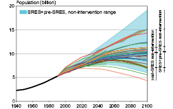
Figure 3.1: Comparison of population assumptions in post-SRES emissions scenarios with those used in previous scenarios. Blue shaded areas span the range of 84 population scenarios used in SRES or pre-SRES emissions scenarios; individual curves show population assumptions in 117 emissions scenarios in the literature since 2000 . The two vertical bars on the right extend from the minimum to maximum of the distribution of scenarios by 2100 . The horizontal bars indicate the 5th, 25th, 50th, 75th and the 95th percentiles of the distributions.
3.2.1.2 Economic development
Economic activity is a dominant driver of energy demand and thus of greenhouse gas emissions. This activity is usually reported as gross domestic product (GDP), often measured in per-person (per-capita) terms. To derive meaningful comparisons over time, changes in price levels must be taken into account and corrected by reporting activities as constant prices taken from a base year. One way of reducing the effects of different base years employed across various studies is to report real growth rates for changes in economic output. Therefore, the focus below is on real growth rates rather than on absolute numbers.
Given that countries and regions use particular currencies, another difficulty arises in aggregating and comparing economic output across countries and world regions. There are two main approaches: using an observed market exchange rate (MER) in a fixed year or using a purchasing power parity rate (PPP) (see Box 3.1 ). GDP trajectories in the large majority of long-term scenarios in the literature are calibrated in MER. A few dozen scenarios exist that use PPP exchange rates, but most of them are shorter-term, generally running until the year 2030 .
3.2.1.3 GDP growth rates in the new literature
Many of the long-term economic projections in the literature have been specifically developed for climate-related scenario work. Figure 3.2 compares the global GDP range of 153 baseline scenarios from the pre-SRES and SRES literature with 130 new scenarios developed since SRES (post-SRES). There is a considerable overlap in the GDP numbers published, with a slight downward shift of the median in the new scenarios (by about 7%) compared to the median in the pre-SRES scenario literature. The data suggests no appreciable change in the distribution of GDP projections.
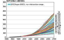
Figure 3.2: Comparison of GDP projections in post-SRES emissions scenarios with those used in previous scenarios. The median of the new scenarios is about 7% below the median of the pre-SRES and SRES scenario literature. The two vertical bars on the right extend from the minimum to maximum of the distribution of scenarios by 2100 . The horizontal bars indicate the 5th, 25th, 50th, 75th and the 95th percentiles of the distributions.
A comparison of some recent shorter-term global GDP projections using the SRES scenarios is illustrated in Figure 3.3 . The SRES scenarios project a very wide range of global economic per-person growth rates from 1% (A2) to 3.1% (A1) to 2030, both based on MER. This range is somewhat wider than that covered by the USDOE 2004 [NPR, MoS] ) high and low scenarios (1.2–2.5%). The central projections of USDOE, IEA and the World Bank all contain growth rates of around 1.5–1.9%, thus occurring in the middle of the range of the SRES scenarios. Other medium-term energy scenarios are also reported to have growth rates in this range ( IEA, 2004 [NPR] ).
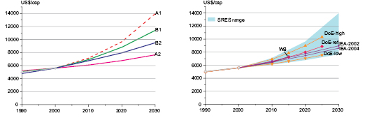
Figure 3.3: Comparison of global GDP growth per person in the SRES scenarios and more recent projections.
Regionally, for the OECD, Eastern Europe and Central Asia (REF) regions, the correspondence between SRES outcomes and recent scenarios is relatively good, although the SRES GDP growth rates are somewhat conservative. In the ASIA region, the SRES range and its median value are just above that of recent studies. The differences between the SRES outcomes and more recent projections are largest in the ALM region (covering Africa, Latin America and the Middle East). Here, the A1 and B1 scenarios clearly lie above the upper end of the range of current projections (4%–5%), while A2 and B2 fall near the centre of the range (1.4–1.7%). The recent short-term projections reported here contain an assumption that current barriers to economic growth in these regions will slow growth, at least until 2015 .
3.2.1.4 The use of MER in economic and emissions scenarios modelling
The uses of MER-based economic projections in SRES have recently been criticized ( (Castles and Henderson, 2003a, ) 2003b; ( Henderson, 2005 ) ). The vast majority of scenarios published in the literature use MER-based economic projections. Some exceptions exist, for example, MESSAGE in SRES, and more recent scenarios using the MERGE model ( Manne and Richels, 2003 [NPR, SRC] ), along with shorter term scenarios to 2030, including the G-Cubed model ( (McKibbin et al., 2004a, ) 2004b ), the International Energy Outlook ( USDOE, 2004 [NPR, MoS] ), the IEA World Energy Outlook ( IEA, 2004 [NPR] ) and the POLES model used by the European Commission ( 2003 ). The main criticism of the MER-based models is that GDP data for world regions are not corrected with respect to purchasing power parities (PPP) in most of the model runs. The implied consequence is that the economic activity levels in non-OECD countries generally appear to be lower than they actually are when measured in PPP units. In addition, the high growth SRES scenarios (A1 and B1 families) assume that regions tend to conditionally converge in terms of relative per-person income across regions (see Section 3.1.4 ). According to the critics, the use of MER, together with the assumption of conditional convergence, lead to overstated economic growth in the poorer regions and excessive growth in energy demand and emission levels.
A team of SRES researchers responded to this criticism, indicating that the use of MER or PPP data does not in itself lead to different emission projections outside the range of the literature. In addition, they stated that the use of PPP data in most scenarios models was (and still is) infeasible, due to lack of required data in PPP terms, for example price elasticities and social accounting matrices ( Nakicenovic et al., 2003 [Ambiguous] ; Grübler et al., 2004 [SRC] ). A growing number of other researchers have also indicated different opinions on this issue or explored it in a more quantitative sense (e.g. Dixon and Rimmer, 2005 [NPR, MoS] ; Nordhaus, 2006b [NPR] ; Manne and Richels, 2003 [NPR, SRC] ;( McKibbin et al., 2004a, ) 2004b; Holtsmark and Alfsen, 2004a [JoC, SRC] , 2004b; van Vuuren and Alfsen, 2006 [JoC, SRC] ).
There are at least three strands to this debate. The first is whether economic projections based on MER are appropriate, and thus whether the economic growth rates reported in the SRES and other MER-based scenarios are reasonable and robust. The second is whether the choice of the exchange rate matters when it comes to emission scenarios. The third is whether it is possible, or practical, to develop robust scenarios given the sparseness of relevant and required PPP data. While the GDP data are available in PPP, other economic scenario characteristics, such as capital and operational cost of energy facilities, are usually available either in domestic currencies or MER. Full model calibration in PPP for regional and global models is still difficult due to the lack of underlying data. This could be one of the reasons why a vast majority of long-term emissions scenarios continues to be calibrated in MER.
On the question of whether PPP or MER should be employed in economic scenarios, the general recommendations are to use PPP where practical. [3] This is certainly necessary when comparisons of income levels across regions are of concern. On the other hand, models that analyse international trade and include trade as part of their economic projections, are better served by MER data given that trade takes place between countries in actual market prices. Thus, the choice of conversion factor depends on the type of analysis or comparison being undertaken.
For principle and practical reasons, Nordhaus 2005 [NPR, MoS] ) recommends that economic growth scenarios should be constructed by using regional or national accounting figures (including growth rates) for each region, but using PPP exchange rates for aggregating regions and updating over time by use of a superlative price index. In contrast, Timmer 2005 [NPR] ) actually prefers the use of MER data in long-term modelling, as such data are more readily available, and many international relations within the model are based on MER. Others (e.g. van Vuuren and Alfsen, 2006 [JoC, SRC] ) also argue that the use of MER data in long-term modelling is often preferable, given that model parameters are usually estimated on MER data and international trade within the models is based on MER. The real economic consequences of the choice of conversion rates will obviously depend on how the scenarios are constructed, as well as on the type of model used for quantifying the scenarios. In some of the short-term scenarios (with a horizon to 2030 ) a bottom-up approach is taken where assumptions about productivity growth and investment/saving decisions are the main drivers of growth in the models (e.g. ( McKibbin et al., 2004a, ) 2004b ). In long-term scenario models, a top-down approach is more commonly used where the actual growth rates are prescribed more directly, based on convergence or other assumptions about long-term growth potentials.
When it comes to emission projections, it is important to note that in a fully disaggregated (by country) multi-sector economic model of the global economy, aggregate index numbers play no role and the choice between PPP and MER conversion of income levels does not arise. However, in an aggregated model with consistent specifications (i.e. where model parameter estimation and model calibrations are all carried out based on consistent use of conversion factors), the effects of the choice of conversion measure on emissions should approximately cancel out. The reason can be illustrated by using the Kaya identity, which decomposes the emissions as follows:
GHG = Population x GDP per person x Emissions per GDP
or:

where GHG stands for greenhouse gas emissions, GDP stands for economic output, and POP stands for population size. [4]
Given this relationship, emission scenarios can be represented, explicitly based on estimates of population development, economic growth, and development of emission intensity.
Population is often projected to grow along a pre-described (exogenous) path, while economic activity and emission intensities are projected based on differing assumptions from scenario to scenario. The economic growth path can be based on historical growth rates, convergence assumptions, or on fundamental growth factors, such as saving and investment behaviour, productivity changes, etc. Similarly, future emission intensities can be projected based on historical experience, economic factors, such as labour productivity or other key factors determining structural changes in an economy, or technological development. The numerical expression of GDP clearly depends on conversion measures; thus GDP expressed in PPP will deviate from GDP expressed in MER, particularly for developing countries. However, when it comes to calculating emissions (or other physical measures such as energy), the Kaya identity shows that the choice between MER-based or PPP-based representations of GDP will not matter, since emission intensity will change (in a compensating manner) when the GDP numbers change. While using PPP values necessitates using lower economic growth rates for developing countries under the convergence assumption, it is also necessary to adjust the relationship between income and demand for energy with lower economic growth, leading to slower improvements in energy intensities. Thus, if a consistent set of metrics is employed, the choice of metric should not appreciably affect the final emission level.
In their modelling work, Manne and Richels 2003 [NPR, SRC] ( and McKibbin et al. 2004a, ) 2004b ) find some differences in emission levels between using PPP-based and MER-based estimates. Analysis of their work indicates that these results critically depend on, among other things, the combination of convergence assumptions and the mathematical approximation used between MER-GDP and PPP-GDP. In the Manne and Richels work for instance, autonomous efficiency improvement (AEI) is determined as a percentage of economic growth and estimated on the basis of MER data. In going from MER to PPP, the economic growth rate declines as expected, leading to a decline in the autonomous efficiency improvement. However, it is not clear whether it is realistic not to change the AEI rate when changing conversion measure. On the other hand, Holtsmark and Alfsen 2004a [JoC, SRC] , 2004b ), showed that in their simple model consistent replacement of the metric (PPP for MER) – for income levels as well as for underlying technology relationships – leads to a full cancellation of the impact of choice of metric on projected emission levels.
To summarize: available evidence indicates that the differences between projected emissions using MER exchange rates and PPP exchange rates are small in comparison to the uncertainties represented by the range of scenarios and the likely impacts of other parameters and assumptions made in developing scenarios, for example, technological change. However, the debate clearly shows the need for modellers to be more transparent in explaining conversion factors, as well as taking care in determining exogenous factors used for their economic and emission scenarios.
Box 3.1 Market Exchange Rates and Purchasing Power Parity
To aggregate or compare economic output from various countries, GDP data must be converted into a common unit. This conversion can be based on observed market exchange (MER) rates or purchasing power parity (PPP) rates where, in the latter, a correction is made for differences in price levels between countries. The PPP approach is considered to be the better alternative if data is used for welfare or income comparisons across countries or regions. Market exchange rates usually undervalue the purchasing power of currencies in developing countries, see Figure 3.4 .
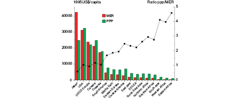
Figure 3.4 : Regional GDP per person, expressed in MER and PPP on the basis of World Bank data aggregated to 17 global regions.
Clearly, deriving PPP exchange rates requires analysis of a relatively large amount of data. Hence, methods have been devised to derive PPP rates for new years on the basis of price indices. Unfortunately, there is currently no single method or price index favoured for doing this, resulting in different sets of PPP rates (e.g. from the OECD, Eurostat, World Bank and Penn World Tables) although the differences tend to be small.
3.2.1.5 Energy use
Future evolution of energy systems is a fundamental determinant of GHG emissions. In most models, energy demand growth is a function of key driving forces such as demographic change and the level and nature of human activities such as mobility, information processing, and industry. The type of energy consumed is also important. While Chapters 4 through 11 report on medium-term projections for different parts of the energy system, long-term energy projections are reported here. Figure 3.5 compares the range of the 153 SRES and pre-SRES scenarios with 133 new, post-SRES, long-term energy scenarios in the literature. The ranges are comparable, with small changes on the lower and upper boundaries, and a shift downwards with respect to the median development. In general, the energy growth observed in the newer scenarios does not deviate significantly from the previous ranges as reported in the SRES report. However, most of the scenarios reported here have not adapted the lower population levels discussed in Section 3.2.1.1 .
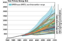
Figure 3.5: Comparison of 153 SRES and pre-SRES baseline energy scenarios in the literature compared with the 133 more recent, post-SRES scenarios. The ranges are comparable, with small changes on the lower and upper boundaries.
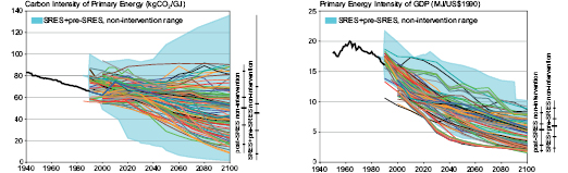
In general, this situation also exists for underlying trends as represented by changes in energy intensity, expressed as gigajoule (GJ)/GDP, and change in the carbon intensity of the energy system (CO2/GJ) as shown in Figure 3.6 . In all scenarios, energy intensity improves significantly across the century – with a mean annual intensity improvement of 1%. The 90% range of the annual average intensity improvement is between 0.5% and 1.9% (which is fairly consistent with historic variation in this factor). Actually, this range implies a difference in total energy consumption in 2100 of more than 300% – indicating the importance of the uncertainty associated with this ratio. The carbon intensity is more constant in scenarios without climate policy. The mean annual long-term improvement rate over the course of the 21st century is 0.4%, while the uncertainty range is again relatively large (from -0.2 to 1.5%). At the high end of this range, some scenarios assume that energy technologies without CO2 emissions become competitive without climate policy as a result of increasing fossil fuel prices and rapid technology progress for carbon-free technologies. Scenarios with a low carbon-intensity improvement coincide with scenarios with a large fossil fuel base, less resistance to coal consumption or lower technology development rates for fossil-free energy technologies. The long-term historical trend is one of declining carbon intensities. However, since 2000, carbon intensities are increasing slightly, primarily due to the increasing use of coal. Only a few scenarios assume the continuation of the present trend of increasing carbon intensities. One of the reasons for this may be that just a few of the recent scenarios include the effects of high oil prices.
3.2.1.6 Land-use change and land-use management
Understanding land-use and land-cover changes is crucial to understanding climate change. Even if land activities are not considered as subject to mitigation policy, the impact of land-use change on emissions, sequestration, and albedo plays an important role in radiative forcing and the carbon cycle.
Over the past several centuries, human intervention has markedly changed land surface characteristics, in particular through large-scale land conversion for cultivation ( Vitousek et al., 1997 [JoC] ). Land-cover changes have an impact on atmospheric composition and climate via two mechanisms: biogeophysical and biogeochemical. Biogeophysical mechanisms include the effects of changes in surface roughness, transpiration, and albedo that, over the past millennium, are thought to have had a global cooling effect ( Brovkin et al., 1999 [MoS] ). Biogeochemical effects result from direct emissions of CO2 into the atmosphere from deforestation. Cumulative emissions from historical land-cover conversion for the period 1920 – 1992 have been estimated to be between 206 and 333 Pg CO2 ( McGuire et al., 2001 [PoC, JoC, MoS] ), and as much as 572 Pg CO2 for the entire industrial period 1850 – 2000, roughly one-third of total anthropogenic carbon emissions over this period ( Houghton, 2003 [NPR, MoS] ). In addition, land management activities (e.g. cropland fertilization and water management, manure management and forest rotation lengths) also affect land-based emissions of CO2 and non-CO2 GHGs, where agricultural land management activities are estimated to be responsible for the majority of global anthropogenic methane (CH4) and nitrous oxide (N2O) emissions. For example, USEPA 2006a [NPR] ) estimated that agricultural activities were responsible for approximately 52% and 84% of global anthropogenic CH4 or N2O emissions respectively in the year 2000, with a net contribution from non-CO2 GHGs of 14% of all anthropogenic greenhouse gas emissions in that year.
Projected changes in land use were not explicitly represented in carbon cycle studies until recently. Previous studies into the effects of future land-use changes on the global carbon cycle employed trend extrapolations ( (Cramer et al., 2004 ) ), extreme assumptions about future land-use changes ( House et al., 2002 [NPR] ), or derived trends of land-use change from the SRES storylines ( Levy et al., 2004 [JoC] ). However, recent studies (e.g. Brovkin et al., 2006 [MoS] ; Matthews et al., 2003 [MoS] ; Gitz and Ciais, 2004 [MoS] ) have shown that land use, as well as feedbacks in the society-biosphere-atmosphere system (e.g. Strengers et al., 2004 [MoS, SRC] ), must be considered in order to achieve realistic estimates of the future development of the carbon cycle; thereby providing further motivation for ongoing development to explicitly model land and land-use drivers in global integrated assessment and climate economic frameworks. For example, in a model comparison study of six climate models of intermediate complexity, Brovkin et al. 2006 [MoS] ) concluded that land-use changes contributed to a decrease in global mean annual temperature in the range of 0.13–0.25°C, mainly during the 19th century and the first half of the 20th century, which is in line with conclusions from other studies, such as Matthews et al. 2003 [MoS] ).
In general, land-use drivers influence either the demand for land-based products and services (e.g. food, timber, bio-energy crops, and ecosystem services) or land-use production possibilities and opportunity costs (e.g. yield-improving technologies, temperature and precipitation changes, and CO2 fertilization). Non-market values – both use and non-use such as environmental services and species existence values respectively – will also shape land-use outcomes.
Food demand is a dominant land-use driver, and population and economic growth are the most significant food demand drivers through per person consumption. Total world food consumption is expected to increase by over 50% by 2030 ( Bruinsma, 2003 [NPR] ). Moreover, economic growth is expected to generate significant structural change in consumption patterns, with diets shifting to include more livestock products and fewer staples such as roots and tubers. As a result, per person meat consumption is expected to show a strong global increase, in the order of 25% by 2030, with faster growth in developing and transitional countries of more than 40% and 30%, respectively ( Bruinsma, 2003 [NPR] ; Cassman et al., 2003 [ARC] ). The Millennium Ecosystem Assessment (MEA) scenarios projected that global average meat consumption would increase from 36 kg/person in 1997 to 41–70 kg/person by 2050, with corresponding increases in overall food and livestock feed demands ( Carpenter et al., 2005 [NPR] ). Additional cropland is expected to be required to support these projected increases in demand. Beyond 2050, food demand is expected to level off with slow-down of population growth.
Technological change is also a critical driver of land use, and a critical assumption in land-use projections. For example, Sands and Leimbach 2003 [JoC, MoS] ) suggest that, globally, 800 million hectares of cropland expansion could be avoided with a 1% annual growth in crop yields. Similarly, Kurosawa 2006 [NPR] ) estimates decreased cropland requirements of 18% by 2050, relative to 2000, with 2% annual growth in global average crop yields. Alternatively, the MEA scenarios implement a more complex representation of yield growth projections that, in addition to autonomous technological change, reflect the changes in production practices, investments, technology transfer, environmental degradation, and climate change. The net effect is positive, but shows declining productivity growth over time for some commodities, due in large part to diminishing marginal technical productivity gains and environmental degradation. In all these studies, increasing (decreasing) net productivity per hectare results in reduced (increased) cropland demand.
Also important to land-use projections are potential changes in climate. For instance, rising temperatures and CO2 fertilization may improve regional crop yields in the short term, thereby reducing pressure for additional cropland and resulting in increased afforestation. However, modelling the beneficial impacts of CO2 fertilization is not as straightforward as once thought. Recent results suggest: lower crop productivity improvements in the field than shown previously with laboratory results (e.g. Ainsworth and Long, 2005 [NPR] ); likely increases in tropospheric ozone and smog associated with higher temperatures that will depress plant growth and partially offset CO2 fertilization; expected increases in the variability of annual yields; CO2 effects favouring C3 plants (e.g. wheat, barley, potatoes, rice) over C4 plants (e.g. maize, sugar cane, sorghum, millet) while temperature increases favour C4 over C3 plants; potential decreased nutritional content in plants subjected to CO2 fertilization and increased frequency of temperature extremes; and increases in forest disturbance frequency and intensity. See IPCC 2007b [NPR, 2007] , Chapter 5 ) for an overall discussion of these issues and this literature. Long-term projections need to consider these issues, as well as examining the potential limitations or saturation points of plant responses. However, to date, long-term scenarios from integrated assessment models are only just beginning to represent climate feedbacks on terrestrial ecosystems, much less fully account for the many effects. Current integrated assessment representations only consider CO2 fertilization and changes in yearly average temperature, if they consider climate change effects at all (e.g. USCCSP, 2006 [NPR] ; van Vuuren et al., 2007 [JoC, SRC, 2007] ).
Only a few global studies have focused on long-term (century) land-use projections. The most comprehensive studies, in terms of sector and land-type coverage, are the SRES ( Nakicenovic et al., 2000 [NPR, SRC] ), the SRES implementation with the IMAGE model ( Strengers et al., 2004 [MoS, SRC] ), the scenarios from the Global Scenarios Group ( Raskin et al., 2002 [NPR, ARC] ), UNEP’s Global Environment Outlook ( UNEP, 2002 [NPR, MoS] ), the Millennium Ecosystem Assessment ( Carpenter et al., 2005 [NPR] ), and some of the EMF-21 Study models ( Kurosawa, 2006 [NPR] ; van Vuuren et al., 2006a [NPR, MoS, SRC] ; Rao and Riahi, 2006 [SRC] ; Jakeman and Fisher, 2006 [NPR, SRC] ; Riahi et al., 2006 [NPR, SRC] ; van Vuuren et al., 2007 [JoC, SRC, 2007] ). Recent sector-specific economic studies have also contributed global land-use projections for climate analysis, especially for forestry ( Sands and Leimbach, 2003 [JoC, MoS] ; Sohngen and Mendelsohn, 2003 [MoS, ARC] , 2007; Sathaye et al., 2006 [NPR, ARC] ; Sohngen and Sedjo, 2006 [NPR, ARC] ). In general, the post-SRES scenarios, though scarce in number for agricultural land use, have projected increasing global cropland areas, smaller forest-land areas, and mixed results for changes in global grassland ( Figure 3.7 ). Unlike the SRES land-use scenarios that span a broader range while representing diverse storylines, the post-SRES scenarios, for forestry in particular, illustrate greater convergence across models on projected land-use change.
Most post-SRES global scenarios project significant changes in agricultural land caused primarily by regional changes in food demand and production technology. Scenarios with larger amounts of land used for agriculture result from assumptions about higher population growth rates, higher food demands, and lower rates of technological improvement that generate negligible increases in crop yields. Combined, these effects are projected to lead to a sizeable expansion (up to 40%) of agricultural land between 1995 and 2100 ( Figure 3.7 ). Conversely, lower population growth and food demand, and more rapid technological change, are projected to result in lower demand for agricultural land (as much as 20% less global agricultural acreage by the end of the century). In the short-term, almost all scenarios suggest an increase in cropland acreage and decline in forest land to meet projected increases in food, feed, and livestock grazing demands over the next few decades. Cropland changes range from -18% to +69% by 2050 relative to 2000 (from -123 to +, (from -123 to +, million hectares) and forest-land changes range from -18% to +3% (from -680 to +94 million hectares) by 2050 . The changes in global forest generally mirror the agricultural scenarios; thereby, illustrating both the positive and negative aspects of some existing global land modelling. Most of the long-term scenarios assume that forest trends are driven almost exclusively by cropland expansion or contraction, and only deal superficially with driving forces, such as global trade in agricultural and forest products and conservation demands.
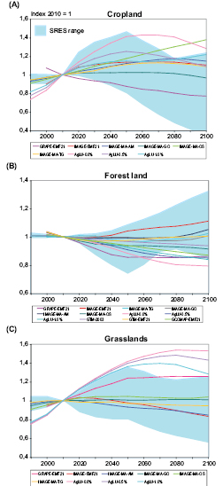
Without incentives or technological innovation, biomass crops are currently not projected to assume a large share of global business as usual land cover – no more than about 4% by 2100 . Until long-run energy price expectations rise (due to a carbon price, economic scarcity, or other force), biomass and other less economical energy supply technologies (some with higher greenhouse gas emission characteristics than biomass), are not expected to assume more significant baseline roles.
3.2.2 Emissions
There is still a large span of CO2 emissions across baseline scenarios in the literature, with emissions in 2100 ranging from 10 GtCO2 to around 250 GtCO2. The wide range of future emissions is a result of the uncertainties in the main driving forces, such as population growth, economic development, and energy production, conversion, and end use, as described in the previous section.
3.2.2.1 CO2 emissions from energy and industry
This category of emissions encompasses CO2 emissions from burning fossil fuels, and industrial emissions from cement production and sometimes feedstocks. [5] Figure 3.8 compares the range of the pre-SRES and SRES baseline scenarios with the post-SRES baseline scenarios. The figure shows that the scenario range has remained almost the same since the SRES. There seems to have been an upwards shift on the high and low end, but careful consideration of the data shows that this is caused by only very few scenarios and the change is therefore not significant. The median of the recent scenario distribution has shifted downwards slightly, from 75 GtCO2 by 2100 (pre-SRES and SRES) to about 60 GtCO2 (post SRES). The median of the recent literature therefore corresponds roughly to emissions levels of the intermediate SRES-B2 scenarios. The majority of scenarios, both pre-SRES and post-SRES, indicate an increase in emissions across most of the century, resulting in a range of 2100 emissions of 17–135 GtCO2 emissions from energy and industry (90th percentile of the full scenario distribution). Also the range of emissions depicted by the SRES scenarios is consistent with the range of other emission scenarios reported in the literature; both in the short and long term (see van Vuuren and O’Neill, 2006 [JoC, MoS, SRC] ).
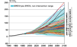
Figure 3.8: Comparison of the SRES and pre-SRES energy-related and industrial CO2 emissions scenarios in the literature with the post-SRES scenarios.
Several reasons may contribute to the fact that emissions have not declined in spite of somewhat lower projections for population and GDP. An important reason is that the lower demographic projections are only recently being integrated into emission scenario literature. Second, indirect impacts in the models are likely to offset part of the direct impacts. For instance, lower energy demand leads to lower fossil fuel depletion, thus allowing for a higher share of fossil fuels in the total energy mix over a longer period of time. Finally, in recent years there has been increasing attention to the interpretation of fossil fuel reserves reported in the literature. Some models may have decreased oil and gas use in this context, leading to higher coal use (and thus higher emissions).
Analysis of scenario literature using the Kaya identity shows that pre-SRES and post-SRES baseline scenarios indicate a continuous decline of the primary energy intensity (EJ/GDP), while the change in carbon intensity (CO2/E) is much slower – or even stable (see Figure 3.6 and Section 3.2.1.5 ) in the post-SRES scenarios. In other words, in the absence of climate policy, structural change and energy efficiency improvement do contribute to lower emissions, but changes in the energy mix have a much smaller (or even zero) contribution. This conclusion is true for both the pre-SRES, SRES, as well as the post-SRES scenario literature.
Baseline or reference emissions projections generally come from three types of studies:
1. Studies meant to represent a ‘best-guess’ of what might happen if present-day trends and behaviour continue.
2. Studies with multiple baseline scenarios under comprehensively different assumptions (storylines).
3. Studies based on a probabilistic approach.
In literature, since the TAR, there has been some discussion of the purpose of these approaches (see Schneider, 2001 [PoC, JoC] ; Grübler et al., 2002 [ARC] ; Webster et al., 2002 [MoS, SRC] ). Figure 3.9 (left panel) shows a comparison of the outcomes of some prominent examples of these approaches by comparing the outcome of baselines scenarios reported in the set of EMF-21 scenarios, representing the ‘best-guess’ approach, to the outcomes of the SRES scenarios, representing the storyline approach. In the right panel the SRES range is compared to the probabilistic approach (see Webster et al., 2002 [MoS, SRC] ; Richels et al., 2004 [NPR, SRC] , for the probability studies).
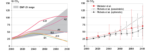
Figure 3.9: Comparison of various long-term scenario studies for CO2 emissions. Left panel: IPCC SRES, EMF-21 range (grey area), indicating the range of the lowest and highest reported values in the EMF-21 study ( Weyant et al., 2006 [NPR, SRC] ). Right panel: Webster et al. 2002 [MoS, SRC] and Richels et al. 2004 [NPR, SRC] ), indicating the mean (markers) and 95% intervals of the reported ranges of these studies (for the latter, showing the 95% interval of the combined range for optimistic and pessimistic technology).
The figure shows that the range of different models participating in the EMF-21 study is somewhat smaller than those from SRES and the probabilistic approach. The range of EMF-21 scenarios result from different modelling approaches and from modeller’s insights into ‘the mostly likely values’ for driving forces. The two probabilistic studies and SRES explicitly assume more radical developments, but the number of studies involved is smaller. This leads to the low end of scenarios for the second category having very specific assumptions on development that may lead to low greenhouse gas emissions. The range of scenarios in the probabilistic studies tends to be between these extremes. Overall, the three different approaches seem to lead to consistent results, confirming the range of emissions reported in Figure 3.8 and confirming the emission range of scenarios used for the TAR.
3.2.2.2 Anthropogenic land emissions and sequestration
Some of the first global integrated assessment scenario analyses to account for land-use-related emissions were the IS92 scenario set ( Leggett et al., 1992 [NPR, ARC] ) and the SRES scenarios ( Nakicenovic et al., 2000 [NPR, SRC] ). However, out of the six SRES models, only four dealt with land use specifically (MiniCAM, MARIA, IMAGE 2.1, AIM), of which MiniCAM and MARIA used more simplified land-use modules. ASF and MESSAGE also simulated land-use emissions, however ASF did not have a specific land-use module and MESSAGE incorporated land-use results from the AIM model ( Nakicenovic et al., 2000 [NPR, SRC] ). Although SRES was a seminal contribution to scenario development, the treatment of land-use emissions was not the focus of this assessment; and, therefore, neither was the modelling of land-use drivers, land management alternatives, and the many emissions sources, sinks, and GHGs associated with land.
While some recent assessments, such as UNEP’s Third Global Environment Outlook ( UNEP, 2002 [NPR, MoS] ) and the Millennium Ecosystem Assessment ( Carpenter et al., 2005 [NPR] ), have evaluated land-based environmental outcomes (global environment and ecosystem goods and services respectively), the Energy Modelling Forum’s 21st Study (EMF-21) was the first large-scale exercise with a special focus on land as a climate issue. In EMF-21, the integrated assessment models incorporated non-CO2 greenhouse gases, such as those from agriculture, and carbon sequestration in managed terrestrial ecosystems ( Kurosawa, 2006 [NPR] ; van Vuuren et al., 2006a [NPR, MoS, SRC] ; Rao and Riahi, 2006 [SRC] ; Jakeman and Fisher, 2006 [NPR, SRC] ). A few additional papers have subsequently improved upon their EMF-21 work ( Riahi et al., 2006 [NPR, SRC] ; van Vuuren et al., 2007 [JoC, SRC, 2007] ). In general, the land-use change carbon emissions scenarios since SRES project high global annual net releases of carbon in the near future that decline over time, leading to net sequestration by the end of the century in some scenarios (see Figure 3.10 ). The clustering of the non-harmonized post-SRES scenarios in Figure 3.10 suggests a degree of expert agreement that the decline in annual land-use change carbon emissions over time will be less dramatic (slower) than suggested by many of the SRES scenarios. Many of the post-SRES scenarios project a decrease in net deforestation pressure over time, as population growth slows and crop and livestock productivity increase; and, despite continued projected loss of forest area in some scenarios ( Figure 3.7 ), carbon uptake from afforestation and reforestation result in net sequestration.
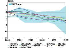
There also seems to be a consensus in recent non-CO2 GHG emission baseline scenarios that agricultural CH4 and N2O emissions will increase until the end of this century, potentially doubling in some baselines (see Table 3.1 Kurosawa, 2006 [NPR] ; van Vuuren et al., 2006a [NPR, MoS, SRC] ; Rao and Riahi, 2006 [SRC] ; Jakeman and Fisher, 2006 [NPR, SRC] ; Riahi et al., 2006 [NPR, SRC] ; van Vuuren et al., 2007 [JoC, SRC, 2007] ). The modelling of agricultural emission sources varies across scenarios, with livestock and rice paddy methane and crop soil nitrous oxide emissions consistently represented. However, the handling of emissions from biomass burning and fossil fuel combustion are inconsistent across models; and cropland soil carbon fluxes are generally not reported, probably due to the fact that soil carbon sequestration mitigation options are not currently represented in these models.
Table 3.1: Baseline global agricultural non-CO2 greenhouse gas emissions from various long-term stabilization scenarios (GtCO2-eq).
| Scenario | Non-CO2 GHG agricultural emissions sources represented* | GtCO2-eq | |||||||||
|---|---|---|---|---|---|---|---|---|---|---|---|
| CH4 | N2O | ||||||||||
| 2000 | 2020 | 2050 | 2070 | 2100 | 2000 | 2020 | 2050 | 2070 | 2100 | ||
| GTEM-EMF21 | Enteric, manure, paddy rice, soil (N2O) | 2.09 | 2.88 | 4.28 | nm | nm | 1.95 | 2.60 | 3.64 | nm | nm |
| MESSAGE-EMF21 | Enteric, manure, paddy rice, soil (N2O) | 2.58 | 3.42 | 6.05 | 6.00 | 5.06 | 2.57 | 3.48 | 4.65 | 3.79 | 2.32 |
| IMAGE-EMF21 | Enteric, manure, paddy rice, soil (N2O and CO2), biomass & agriculture waste burning, land clearing | 3.07 | 4.15 | 4.34 | 4.37 | 4.55 | 2.02 | 2.75 | 3.11 | 3.23 | 3.27 |
| GRAPE-EMF21 | Enteric, manure, paddy rice, soil (N2O), biomass & agricultural waste burning | 2.59 | 2.65 | 2.85 | 2.82 | 2.76 | 2.79 | 3.31 | 3.84 | 3.93 | 4.06 |
| MESSAGE-A2r | Enteric, manure, paddy rice, soil (N2O) | 2.58 | 3.43 | 4.78 | 5.52 | 6.57 | 2.57 | 3.48 | 4.37 | 4.77 | 5.22 |
| IMAGE 2.3 | Enteric, manure, paddy rice, soil (N2O and CO2), biomass & agricultural waste burning, land clearing | 3.36 | 3.95 | 4.41 | 4.52 | 4.46 | 2.05 | 2.48 | 2.93 | 3.07 | 3.06 |
As noted in Section 3.2.1.6 climate change feedbacks could have a significant influence on long-term land use and, to date, are only partially represented in long-term modelling of land scenarios. Similarly, climate feedbacks can also affect land-based emissions. For instance, rising temperatures and CO2 fertilization can influence the amount of carbon that can be sequestered by land and may also lead to increased afforestation due to higher crop yields. Climate feedbacks in the carbon cycle could be extremely important. For instance, Leemans et al. 2002 [SRC] ) showed that CO2 fertilization and soil respiration could be as important as the socio-economic drivers in determining the land-use emissions range.
In addition, potentially important additional climate feed-backs in the carbon-climate system are currently not accounted for in integrated assessment scenarios. Specifically, new in-sights suggest that soil drying and forest dieback may naturally reduce terrestrial carbon sequestration ( Cox et al., 2000 [JoC, MoS] ). However, these studies, as well as studies that try to capture changes in climate due to land-use change ( Sitch et al., 2005 [JoC, MoS, SRC] ) have thus far not been able to provide definitive guidance. A modelling system that fully couples land use change scenarios with a dynamic climate-carbon system is required in the future for such an assessment.
3.2.2.3 Non-CO2 greenhouse gas emissions
The emissions scenario chapter in the TAR ( Morita et al., 2001 [NPR, SRC] ) recommended that future research should include GHGs other than CO2 in new scenarios work. The reason was that, at that time, certainly regarding mitigation, most of the scenarios literature was still primarily focused on CO2 emissions from energy. Nevertheless, some multi-gas scenario work existed, including the SRES baseline scenarios, but also some other modelling efforts ( Manne and Richels, 2001 [JoC, SRC] ; Babiker et al., 2001 [NPR, MoS, SRC] ;( Tol, 1999 ) ). The most important non-CO2 gases include: methane (CH4), nitrous oxide (N2O), and a group of fluorinated compounds (F-gases, i.e., HFCs, PFCs, and SF6). Since the TAR, the number of modelling groups producing long-term emission scenarios for non-CO2 gases has dramatically increased. As a result, the quantity and quality of non-CO2 emissions scenarios has improved appreciably.
Unlike CO2 where the main emissions-related sectors are few (i.e. energy, industry, and land use), non-CO2 emissions originate from a larger and more diverse set of economic sectors. Table 3.2 provides a list of the major GHG emitting sectors and their corresponding emissions, estimated for 2000 . Note that there is significant uncertainty concerning emissions from some sources of the non-CO2 gases, and the table summarizes the central values from Weyant et al. 2006 [NPR, SRC] ) which has been used in long-term multi-gas scenario studies of the EMF-21. To make the non-CO2 emissions comparable to those of CO2, the common practice is to compare and aggregate emissions by using global warming potentials (GWPs).
Table 3.2: Global Anthropogenic GHG Emissions for 2000 at sector level, as used in EMF-21 studies (MtCO2-eq/yr).
| Sector sub-total & percent of total | Sub-sectors | CO2 | CH4 | N2O | F-gases |
|---|---|---|---|---|---|
| ENERGY | Coal | 8,133 | 451 | ||
| Natural gas | 4,800 | 895 | |||
| 25,098 | Petroleum syst. | 10,476 | 62 | ||
| 67% | Stationary/Mobile sources | 59 | 224 | ||
| LUCFa and AGRICULTURE | LUCF and agriculture (net) | 3,435 | |||
| Soils | 2,607 | ||||
| Biomass | 491 | 187 | |||
| 9,543 | Enteric fermentationManure management | 1,745224 | -205 | ||
| 25% | Rice | 649 | - | ||
| INDUSTRY | Cement | 829 | |||
| Adipic & nitric acid productionHFC-23 | 158 | 95 | |||
| 1,434 | PFCsSF6 | 10655 | |||
| 4% | Substitution of ODSb | 191 | |||
| WASTE | Landfills | 781 | |||
| 1,448 | Wastewater | 565 | 81 | ||
| 4% | Other | 11 | 11 | ||
| Total all GHG | 37,524 | 27,671 | 5,933 | 3,472 | 447 |
| Gas as percent of total | 74% | 16% | 9% | 1% |
The most important work on non-CO2 GHG emissions scenarios has been done in the context of EMF-21 ( De la Chesnaye and Weyant, 2006 [SRC] ). The EMF-21 study updated the capability of long-term integrated assessment models for modelling non-CO2 GHG emissions. The results of the study are illustrated in Figure 3.11 .
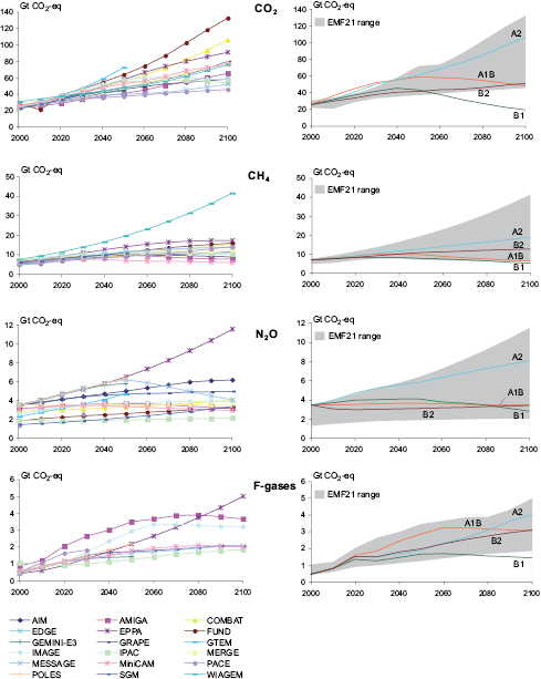
Figure 3.11: Development of baseline emissions in the EMF-21 scenarios (left) and comparison between EMF21 and SRES scenarios (right).
Evaluating the long-term projections of anthropogenic methane emissions from the EMF-21 data shows a significant range in the estimates, but this range is consistent with that found in the SRES. The methane emission differences in the SRES are due to the different storylines. The differences in the EMF-21 reference cases are mainly due to changes in the economic activity level projected in key sectors by each of the models [6] . This could include, for example, increased agriculture production or increased supply of natural gas and below-ground coal in the energy sector. In addition, different modelling groups employed various methods of representing methane emissions in their models and also made different assumptions about how specific methane emission factors for each economic sector change over time. Finally, the degree to which agricultural activities are represented in the models differs substantially. For example, some models represent all agricultural output as one large commodity, ‘agriculture’, while others have considerable disaggregation. Interestingly, the latter group of models tend to find slower emissions growth rates (see van Vuuren et al., 2006b [MoS, SRC] ).
The range of long-term projections of anthropogenic nitrous oxide emissions is wider than for methane in the EMF-21 data. Note that for N2O, base year emissions of the different models differ substantially. Two factors may contribute to this. First, different definitions exist as to what should be regarded as human-induced and natural emissions in the case of N2O emissions from soils. Second, some models do not include all emission sources.
The last group of non-CO2 gases are fluorinated compounds, which include hydrofluorocarbons (HFCs), perfluorocarbons (PFCs), and sulphur hexafluoride (SF6). The total global emissions of these gases are almost 450 MtCO2-eq, or slightly over 1% of all GHG for 2000 . While the emissions of some fluorinated compounds are projected to decrease, many are expected to grow substantially because of the rapid growth rate of some emitting industries (e.g. semiconductor manufacture and magnesium production and processing), and the replacement of ozone-depleting substances (ODSs) with HFCs. Long-term projections of these fluorinated GHGs are generated by a fewer number of models, but still show a wide range in the results over the century. Total emissions of non-CO2 GHGs are projected to increase, but somewhat less rapidly than CO2 emissions, due to agricultural activities growing less than energy use.
3.2.2.4 Scenarios for air pollutants and other radiative substances
Sulphur dioxide emission scenarios
Sulphur emissions are relevant for climate change modelling as they contribute to the formation of aerosols, which affect precipitation patterns and, taken together, reduce radiative forcing. Sulphur emissions also contribute to regional and local air pollution. Global sulphur dioxide emissions have grown approximately in parallel with the increase in fossil fuel use ( Smith et al., 2001 [SRC] , 2004; ( Stern, 2005 ) ). However, since around the late 1970 s, the growth in emissions has slowed considerably ( Grübler, 2002 [ARC] ). Implementation of emissions controls, a shift to lower sulphur fuels in most industrialized countries, and the economic transition process in Eastern Europe and the Former Soviet Union have contributed to the lowering of global sulphur emissions ( Smith et al., 2001 [SRC] ). Conversely, with accelerated economic development, the growth of sulphur emissions in many parts of Asia has been high in recent decades, although growth rates have moderated recently ( (Streets et al., 2000; ) ( Stern, 2005; ) Cofala et al., 2006 [NPR, ARC] ; Smith et al., 2004 [NPR] ). A review of the recent literature indicates that there is some uncertainty concerning present global anthropogenic sulphur emissions, with estimates for the year 2000 ranging between 55.2 MtS ( (Stern, 2005 ) ), 57.5 MtS ( Cofala et al., 2006 [NPR, ARC] ) and 62 MtS ( Smith et al., 2004 [NPR] ). [7]
Many empirical studies have explored the relationship between sulphur emissions and related drivers, such as economic development (see for example, Smith et al., 2004 [NPR] ). The main driving factors that have been identified are increasing income, changes in the energy mix, and a greater focus on air pollution abatement (as a consequence of increasing affluence). Together, these factors may result in an inverted U-shaped pattern of SO2 emissions, where emissions increase during early stages of industrialization, peak and then fall at higher levels of income, following a Kuznets curve (World Bank, 1992 [NPR] ). This general trend is also apparent in most of the recent emissions scenarios in the literature.
Over time, new scenarios have generally produced lower SO2 emissions projections. A comprehensive comparison of the SRES and more recent sulphur-emission scenarios is given in van Vuuren and O’Neill 2006 [JoC, MoS, SRC] ). Figure 3.12 illustrates that the resulting spread of sulphur emissions over the medium term (up to the year 2050 ) is predominantly due to the varying assumptions about the timing of future emissions control, particularly in developing countries [8] . Scenarios at the lower boundary assume the rapid introduction of sulphur-control technologies on a global scale, and hence, a reversal of historical trends and declining emissions in the initial years of the scenario. Conversely, the upper boundaries of emissions are characterized by a rapid increase over coming decades, primarily driven by the increasing use of coal and oil at relatively low levels of sulphur control (SRES A1 and A2).
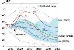
The comparison shows that overall the SRES scenarios are fairly consistent with recent projections concerning the long-term uncertainty range ( Smith et al., 2004 [NPR] ; see Figure 3.12 ). However, the emissions peak over the short-term of some high emissions scenarios in SRES, which lie above the upper boundary estimates of the recent scenarios. There are two main reasons for this difference. First, recent sulphur inventories for the year 2000 have shifted downward. Second, and perhaps more importantly, new information on present and planned sulphur legislation in some developing countries, such as India ( Carmichael et al., 2002 [ARC] ) and China ( Streets et al., 2001 [JoC, SRC] ) has become available. Anticipating this change in legislation, recent scenarios project sulphur emissions to peak earlier and at lower levels compared to the SRES. Also the lower boundary projections of the recent literature have shifted downward slightly compared to the SRES scenario.
NOx emission scenarios
The most important sources of NOx emissions are fossil fuel combustion and industrial processes, which combined with other sources such as natural and anthropogenic soil release, biomass burning, lightning, and atmospheric processes, amount to around 25 MtN per year. Considerable uncertainties exist, particularly around the natural sources ( Prather et al., 1995 [NPR, MoS] ; Olivier et al., 1998 [NPR, ARC] ; Olivier and Berdowski, 2001 [NPR, ARC] ; Cofala et al. 2006 [NPR, ARC] ). Fossil fuel combustion in the electric power and transport sectors is the largest source of NOx, with emissions largely being related to the combustion practice. In recent years, emissions from fossil fuel use in North America and Europe are either constant or declining. Emissions have been increasing in most parts of Asia and other developing parts of the world, mainly due to the growing transport sector ( Cofala et al., 2006 [NPR, ARC] ; Smith, 2005 [MoS] ; WBCSD, 2004 [NPR] ). However in the longer term, most studies project that NOx emissions in developing countries will saturate and eventually decline, following the trend in the developed world. However, the pace of this trend is uncertain. Emissions are projected to peak in the developing world as early as 2015 ( WBCSD, 2004 [NPR] , focusing on the transport sector) and, in worst cases, around the end of this century (see the high emissions projection of Smith, 2005 [MoS] ).
There have been very few global scenarios for NOx emissions since the earlier IS92 scenarios and the SRES. An important characteristic of these (baseline) scenarios is that they consider air pollution legislation (in the absence of any climate policy). Some scenarios, such as those by Bouwman and van Vuuren 1999 [NPR, SRC] ( and Collins et al. 2000 ) ) often use IS92a as a ‘loose’ baseline, with new abatement policies added. Many scenarios report rising NOx emissions up to the 2020 s ( Figure 3.13 ), with the lower boundary given by the short-term Cofala et al. 2006 [NPR, ARC] ) reference scenario, projecting emissions to stay at about present levels for the next two to three decades. In the most recent longer-term scenarios ( Smith, 2005 [MoS] ), NOx emissions range between 32 MtN and 47 MtN by 2020, which corresponds to an increase in emissions of around 6–50% compared to 2000 . The long-term spread is considerably larger, ranging from 9 MtN to 74 MtN by 2100 (see Figure 3.13 ). The majority of the SRES scenarios (70%) lie within the range of the new Smith 2005 [MoS] ) scenarios. However, the upper and lower boundaries of the range of the recent projections have shifted downward compared to the SRES.
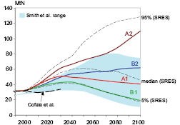
Emission scenarios for black and organic carbon
Black and organic carbon emissions (BC and OC) are mainly formed by incomplete combustion, as well as from gaseous precursors ( (Penner et al., 1993; ) ( Gray and Cass, 1998 ) ). The main sources of BC and OC emissions include fossil fuel combustion in industry, power generation, traffic and residential sectors, as well as biomass and agriculture waste burning. Natural sources, such as forest fires and savannah burning, are other major contributors. There has recently been some research suggesting that carbonaceous aerosols may contribute to global warming ( Hansen et al., 2000 [JoC] ; Andrae, 2001 [JoC] ; Jacobson, 2001 [JoC] ; Ramaswamy et al., 2001 [NPR, PoC, MoS] ). However, the uncertainty concerning the effects of BC and OC on the change in radiative forcing and hence global warming is still high (see Jacobson, 2001 [JoC] ; and Penner et al., 2004 [JoC, MoS] ).
In the past, BC and OC emissions have been poorly represented in economic and systems engineering models due to unavailability of data. For example, in the IPCC’s Third Assessment Report, BC and OC estimates were developed by using CO emissions ( IPCC, 2001b [NPR] ). One of the main reasons for this has been the lack of adequate global inventories for different emission sources. However, some detailed global and regional emission inventories of BC and OC have recently become available ( Table 3.3 ). In addition, some detailed regional inventories are also available including Streets et al. 2003 [JoC] and Kupiainen and Klimont 2004 [NPR] ). While many of these are comprehensive with regard to detail, considerable uncertainty still exists in the inventories, mainly due to the variety in combustion techniques for different fuels as well as measurement techniques. In order to represent these uncertainties, some studies, such as Bond et al. 2004 [JoC] ), provide high, low and ‘best-guess’ values.
Table 3.3: Emission inventories for black and organic carbon (Tg/yr).
| Source | Estimate year | Black carbon | Organic carbon |
|---|---|---|---|
| Penner et al., 1993 | 1980 | 13 | - |
| Cooke and Wilson, 1996 | 1984 | 14a) | - |
| Cooke et al., 1999 | 1984 | 5-6.6a) | 7-10a) |
| Bond et al., 2004 | 1996 | 4.7 (3-10) | 8.9 (5-17) |
| Liousse et al.,1996 | 12.3 | 81 | |
| Junker and Liousse, 2006 | 1997 | 5.7 | 9.5 |
The development in the inventories has resulted in the possibility of estimating future BC and OC emissions. Streets et al. 2004 [JoC, MoS] ) use the fuel-use information and technological change in the SRES scenarios to develop estimates of BC and OC emissions from both contained combustion as well as natural sources for all the SRES scenarios until 2050 Rao et al. 2005 [SRC] and Smith and Wigley 2006 [NPR] ) estimate BC and OC emissions until 2100 for two IPCC SRES scenarios, with an assumption of increasing affluence leading to an additional premium on local air quality. Liousse et al. 2005 [NPR] ) use the fuel-mix and other detail in various energy scenarios and obtain corresponding BC and OC emissions.
The inclusion of technological development is an important factor in estimating future BC and OC emissions because, even though absolute fossil fuel use may increase, a combination of economic growth, increased environmental consciousness, technology development and legislation could imply decreased pollutant emissions ( Figure 3.14 Liousse et al. 2005 [NPR] ) neglect the effects of technological change leading to much higher emission estimates for BC emissions in the long-term in some cases, as compared to other studies such as Streets et al. 2004 [JoC, MoS] Rao et al. 2005 [SRC] and Smith and Wigley 2006 [NPR] ), all of which show declining emissions in the long-term. Another important factor that Rao et al. 2005 [SRC] ) also account for is current and proposed environmental legislation. This suggests the necessity for technology-rich frameworks that capture structural and technological change, as well as policy dynamics in the energy system in order to estimate future BC and OC emissions.
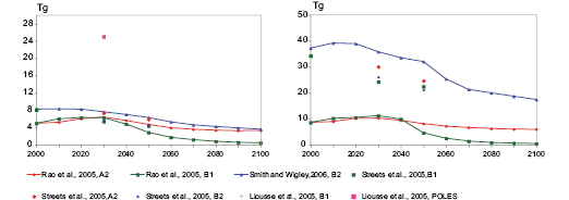
Figure 3.14: Total black carbon (left panel) and organic carbon (right panel) emission estimates in scenarios from different studies.
Streets et al. 2004 [JoC, MoS] and Rao et al. 2005 [SRC] ) show a general decline in BC and OC emissions in developed countries, as well as in regions such as East Asia (including China). In other developing regions, such as Africa and South Asia, slower technology penetration rates lead to much lower emission reductions. There is a large decline in emissions from the residential sector in the developing countries, due to the gradual replacement of traditional fuels and technologies with more efficient ones. Transport-related emissions in both industrialized and developing countries decline in the long-term due to stringent regulations, technology improvements and fuel switching.
To summarize, an important feature of the recent scenario literature is the long-term decline in BC/OC emission intensities per unit of energy use (or economic activity). The majority of the above studies thus indicate that the long-term BC and OC emissions might be decoupled from the trajectory of CO2 emissions.
3.3 Mitigation scenarios
3.3.1 Introduction
This section contains a discussion of methodological issues (Sections 3.3.2 – 3.3.4 ), followed by a focus on the main characteristics of different groups of mitigation scenarios, with specific attention paid to new literature on non-CO2 gases and land use (Sections 3.3.5.5 and 3.3.5.6 ). Finally, short-term scenarios with a regional or national focus are discussed in Section 3.3.6 .
3.3.2 Definition of a stabilization target
Mitigation scenarios explore the feasibility and costs of achieving specified climate change or emissions targets, often in comparison to a corresponding baseline scenario. The specified target itself is an important modelling and policy issue. Because Article 2 of United Nations Framework Convention on Climate Change (UNFCCC) states as its objective the ‘stabilization of greenhouse gas concentrations in the atmosphere at a level that would prevent dangerous anthropogenic interference with the climate system’, most long-term mitigation studies have focused their efforts on GHG concentration stabilization scenarios. However, several other climate change targets may be chosen, for example the rate of temperature change, radiative forcing, or climate change impacts (see e.g. Richels et al., 2004 [NPR, SRC] ; van Vuuren et al., 2006b [MoS, SRC] ; Corfee-Morlot et al., 2005 [JoC] ). In general, selecting a climate policy target early in the cause-effect chain of human activities to climate change impacts, such as emissions stabilization, increases the certainty of achieving required reduction measures, while increasing the uncertainty on climate change impacts (see Table 3.4 ). Selecting a climate target further down the cause-effect chain (e.g. temperature change, or even avoided climate impacts) provides for greater specification of a desired climate target, but decreases certainty of the emission reductions required to reach that target.
Table 3.4: Advantages and disadvantages of using different stabilization targets.
| Target | Advantages | Disadvantages |
|---|---|---|
| Mitigation costs | Lowest uncertainty on costs. | Very large uncertainty on global mean temperature increase and impacts. Very large uncertainty on global mean temperature increase and impacts. Either needs a different metric to allow for aggregating different gases (e.g. GWPs) or forfeits opportunity of substitution. |
| Emissions mitigation | Lower uncertainty on costs. | Does not allow for substitution among gases, thus losing the opportunity for multi-gas cost reductions. Indirect link to the objective of climate policy (e.g. impacts). |
| Concentrations of different greenhouse gases | Can be translated relatively easily into emission profiles (reducing uncertainty on costs). | Allows a wide range of CO2-only stabilization targets due to substitutability between CO2 and non-CO2 emissions. |
| Radiative forcing | Easy translation to emission targets, thus not including climate sensitivity in costs calculations. Does allow for full flexibility in substitution among gases. Connects well to earlier work on CO2 stabilization. Can be expressed in terms of CO2-eq concentration target, if preferred for communication with policymakers. | Indirect link to the objective of climate policy (e.g. impacts). |
| Global mean temperature | Metric is also used to organize impact literature; and as has shown to be a reasonable proxy for impacts | Large uncertainty on required emissions reduction as result of the uncertainty in climate sensitivity and thus costs. |
| Impacts | Direct link to objective of climate polices. | Very large uncertainties in required emission reductions and costs. |
A commonly used target has been the stabilization of the atmospheric CO2 concentration. If more than one GHG is included, most studies use the corresponding target of stabilizing radiative forcing, thereby weighting the concentrations of the different gases by their radiative properties. The advantage of radiative forcing targets over temperature targets is that the consequences for emission trajectories do not depend on climate sensitivity, which adds an important uncertainty. The disadvantage is that a wide range of temperature impacts is possible for each radiative forcing level. By contrast, temperature targets provide a more direct first-order indicator of potential climate change impacts, but are less practical to implement in the real world, because of the uncertainty about the required emissions reductions.
Another approach is to calculate risks or the probability of exceeding particular values of global annual mean temperature rise (see also Table 3.9 ). For example, den Elzen and Meinshausen 2006 [NPR, ARC] and Hare and Meinshausen 2006 [JoC, ARC] ) used different probability density functions of climate sensitivity in the MAGICC simple climate model to estimate relationships between the probability of achieving climate targets and required emission reductions. Studies by Richels et al. 2004 [NPR, SRC] Yohe et al. 2004 [JoC, MoS] den Elzen et al. 2006 [Ambiguous] Keppo et al. 2006 [NPR, MoS, SRC] and Kypreos 2006 [NPR, MoS] ) have used a similar probabilistic concept in an economic context. The studies analyze the relationship between potential mitigation costs and the increase in probability of meeting specific temperature targets.
The choice of different targets is not only relevant because it leads to different uncertainty ranges, but also because it leads to different strategies. Stabilization of one type of target, such as temperature, does not imply stabilization of other possible targets, such as rising sea levels, radiative forcing, concentrations or emissions. For instance, a cost-effective way to stabilize temperature is not radiative forcing stabilization, but rather to allow radiative forcing to peak at a certain concentration, and then decrease with additional emissions reductions so as to avoid (delayed) further warming and stabilize global mean temperature (see Meinshausen, 2006 [NPR, MoS] ; Kheshgi et al., 2005 [ARC] ; den Elzen et al., 2006 [Ambiguous] ). Finally, targets can also be defined to limit a rate of change, such as the rate of temperature change. While such targets have the advantage of providing a link to impacts related to the rate of climate change, strategies to achieve them may be more sensitive to uncertainties and thus, require careful planning. The rate of temperature change targets, for instance, may be difficult to achieve in the short-term even, using multi-gas approaches ( Manne and Richels, 2006 [NPR, SRC] ; van Vuuren et al., 2006a [NPR, MoS, SRC] ).
3.3.3 How to define substitution among gases
In multi-gas studies, a method is needed to compare different greenhouse gases with different atmospheric lifetimes and radiative properties. Ideally, the method would allow for substitution between gases in order to achieve mitigation cost reductions, although it may not be suitable to ensure equivalence in measuring climate impact. Fuglestvedt et al. 2003 [JoC, MoS] ) provide a comprehensive overview of the different methods that have been proposed, along with their advantages and disadvantages. One of these methods, CO2-eq emissions based on Global Warming Potentials (GWP), has been adopted by current climate policies, such as the Kyoto Protocol and the US climate policy White House, 2002 [NPR] ). Despite the continuing scientific and economic debate on the use of GWPs (i.e. they are not based on economic considerations and use an arbitrary time horizon) the concept is in use under the UNFCCC, the Kyoto Protocol, and the US climate policy. In addition, no alternative measure has attained comparable status to date.
Useful overviews of the mitigation and economic implication of substitution metrics are provided by Bradford 2001 [JoC] ( and Godal 2003 ) ). Models that use inter-temporal optimization can avoid the use of substitution metrics (such as GWPs) by optimizing the reductions of all gases simultaneously under a chosen climate target. Inter-temporal optimization or perfect foresight models assume that economic agents know future prices and make decisions to minimize costs. Manne and Richels 2001 [JoC, SRC] ) show, using their model, that using GWPs as the basis of substitution did not lead to the cost-optimal path (minimizing welfare losses) for the long-term targets analyzed. In particular, reducing methane early had no benefit for reaching the long-term target, given its short lifespan in the atmosphere. In the recent EMF-21 study some models validated this result (see de la Chesnaye and Weyant, 2006 [SRC] ). Figure 3.15 shows the projected EMF-21 CO2, CH4, N2O, and F-gas reductions across models stabilizing radiative forcing at 4.5 W/m2. Most of the EMF-21 models based substitution between gases on GWPs. However, three models substituted gases on the basis of inter-temporal optimization. While (for most of the gases) there are no systematic differences between the results from the two groups, for methane and some F-gases (not shown), there are clear differences related to the very different lifespans of these gases. The models that do not use GWPs, do not substantially reduce CH4 until the end of the time horizon. However, for models using GWPs, the reduction of CH4 emissions in the first three decades is substantial: here, CH4 reductions become a cost-effective short-term abatement strategy, despite the short lifespan ( Van Vuuren et al., 2006b [MoS, SRC] ). It should be noted that if a short-term climate target is selected (e.g. rate of temperature change) then inter-temporal optimization models would also favour early methane reductions.
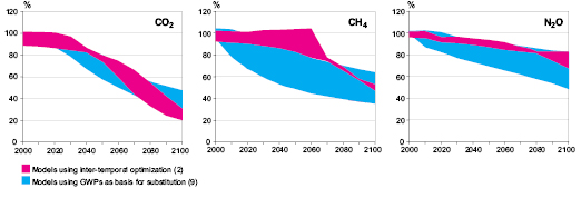
Figure 3.15: Reduction of emissions in the stabilization strategies aiming for stabilization at 4.5 W/m2 (multi-gas strategies) in EMF-21.
While GWPs do not necessarily lead to the most cost-effective stabilization solution (given a long-term target), they can still be a practical choice: in real-life policies an exchange metric is needed to facilitate emissions trading between gases within a specified time period. Allowing such exchanges creates the opportunity for cost savings through ‘what and where flexibility’. It is appropriate to ask what are the costs of using GWPs versus not using them and whether other ‘real world’ metrics exist that could perform better. O’Neill 2003 [JoC, SRC] and Johansson et al. 2006 [JoC] ) have argued that the disadvantages of GWPs are likely to be outweighed by the advantages, by showing that the cost difference between a multi-gas strategy and a CO2-only strategy is much larger than the difference between a GWP-based multi-gas strategy and a cost-optimal strategy. Aaheim et al. 2006 [NPR] ) found that the cost of using GWPs compared to optimal weights, depends on the ambition of climate policies. Postponing the early CH4 reductions of the GWP-based strategy, as is suggested by inter-temporal optimization, generally leads to larger temperature increases during the 2000 – 2020 period. This is because the increased reduction of CO2 from the energy sector also leads to reduction of sulphur emissions (hence the cooling associated with sulphur-based aerosols) but allows the potential to be used later in the century.
3.3.4 Emission pathways
Emission pathway studies often focus on specific questions with respect to the consequences of timing (in terms of environmental impacts) or overall reduction rates needed for specific long-term targets, (e.g. the emission pathways developed by Wigley et al., 1996 [JoC, SRC] ). A specific issue raised in the literature on emission pathways since the TAR has concerned a temporary overshoot of the target (concentration, forcing, or temperature). Meinshausen 2006 [NPR, MoS] ) used a simple carbon-cycle model to illustrate that for low-concentration targets (i.e. below 3 W/m2/ 450 ppmv CO2-eq) overshoot is inevitable, given the feasible maximum rate of reduction. Wigley 2003 [NPR, MoS] ) argued that overshoot profiles may give important economic benefits. In response, O’Neill and Oppenheimer 2004 [SRC] ) showed that the associated incremental warming of large overshoots may significantly increase the risks of exceeding critical climate thresholds to which ecosystems are known to be able to adapt. Other emission pathways that lead to less extreme concentration overshoots may provide a sensible compromise between these two results. For instance, the ‘peaking strategies’ chosen by den Elzen et al. 2006 [Ambiguous] ) show that it is possible to increase the likelihood of meeting the long-term temperature target or to reach targets with a similar likelihood at lower costs. Similar arguments for analyzing overshoot strategies are made by Harvey 2004 [JoC] and Kheshgi et al. 2005 [ARC] ).
3.3.5 Long-term stabilization scenarios
A large number of studies on climate stabilization have been published since the TAR. Several model comparison projects contributed to the new literature, including the Energy Modelling Forum’s EMF-19 ( Weyant, 2004 [SRC] ) and EMF-21 studies ( De la Chesnaye and Weyant, 2006 [SRC] ), that focused on technology change and multi-gas studies, respectively, the IMCP (International Model Comparison Project), which focused on technological change ( Edenhofer et al., 2006 [NPR, ARC] ), and the US Climate Change Science Programme ( USCCSP, 2006 [NPR] ). The updated emission scenario database ( Hanaoka et al., 2006 [NPR, SRC] ; Nakicenovic et al., 2006 [SRC] ) includes a total of 151 new mitigation scenarios published since the SRES.
Comparison of mitigation scenarios is more complicated now than at the time of the TAR because:
- Parts of the modelling community have expanded their analysis to include non-CO2 gases, while others have continued to focus solely on CO2. As discussed in the previous section, multi-gas mitigation scenarios use different targets, thus making comparison more complicated.
- Some recent studies have developed scenarios that do not stabilize radiative forcing (or temperature) – but show a peak before the end of the modelling time horizon (in most cases 2100).
- At the time of the TAR, many studies used the SRES scenarios as baselines for their mitigation analyses, providing a comparable set of assumptions. Now, there is a broader range of underlying assumptions.
This section introduces some metrics to group the CO2-only and multi-gas scenarios so that they are reasonably comparable. In Figure 3.16 the reported CO2 concentrations in 2100 are plotted against the 2100 total radiative forcing (relative to pre-industrial times). Figure 3.16 shows that a relationship exists between the two indicators. This can be explained by the fact that CO2 forms by far the most important contributor to radiative forcing – and subsequently, a reduction in radiative forcing needs to coincide with a reduction in CO2 concentration. The existing spread across the studies is caused by several factors, including differences in the abatement rate among alternative gases, differences in specific forcing values for GHGs and other radiative gases (particularly aerosols), and differences in the atmospheric chemistry and carbon cycle models that are used. Here, the relationship is used to classify the available mitigation literature into six categories that vary in the stringency of the climate targets. The most stringent group includes those scenarios that aim to stabilize radiative forcing below 3 W/m2. This group also includes all CO2-only scenarios that stabilize CO2 concentrations below 400 ppmv. In contrast, the least stringent group of mitigation scenarios have a radiative forcing in 2100 above 6 W/m2 – associated with CO2 concentrations above 660 ppmv. By far the most studied group of scenarios are those that aim to stabilize radiative forcing at 4–5 W/m2 or 485–570 ppmv CO2 (see Table 3.5 ).
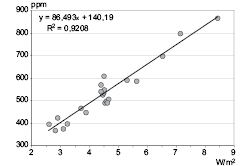
Figure 3.16: Relationship of total radiative forcing vis-à-vis CO2 concentration for the year 2100 (25 multi-gas stabilization scenarios for alternative stabilization targets).
The classification of scenarios, as given in Table 3.5 , permits the comparison of multi-gas and CO2-only stabilization scenarios according to groups of scenarios with comparable level of mitigation stringency. The studies have been classified on the basis of the reported targets, using the relationship from Figure 3.16 to permit comparability of studies using different stabilization metrics. The following section uses these categories (I to VI) to analyze the underlying dynamics of stabilization scenarios as a function of the stabilization target. However, it should be noted that the classification is subject to uncertainty and should thus to be used with care.
Table 3.5: Classification of recent (post-TAR) stabilization scenarios according to different stabilization targets and alternative stabilization metrics. Groups of stabilization targets were defined using the relationship in Figure 3.16 .
| Category | Additional radiative forcing | CO2 concentration | CO2-eq concentration | Peaking year for CO2 emissionsa | Change in global emissions in 2050 (% of 2000 emissions)1 | No. of scenarios |
|---|---|---|---|---|---|---|
| W/m2 | ppm | ppm | year | % | ||
| I | 2.5-3.0 | 350-400 | 445-490 | 2000-2015 | -85 to -50 | 6 |
| II | 3.0-3.5 | 400-440 | 490-535 | 2000-2020 | -60 to -30 | 18 |
| III | 3.5-4.0 | 440-485 | 535-590 | 2010-2030 | -30 to +5 | 21 |
| IV | 4.0-5.0 | 485-570 | 590-710 | 2020-2060 | +10 to +60 | 118 |
| V | 5.0-6.0 | 570-660 | 710-855 | 2050-2080 | +25 to +85 | 9 |
| VI | 6.0-7.5 | 660-790 | 855-1130 | 2060-2090 | +90 to +140 | 5 |
| Total | 177 |
3.3.5.1 Emission reductions and timing
Figure 3.17 shows the projected CO2 emissions associated with the new mitigation scenarios. In addition, the figure depicts the range of the TAR stabilization scenarios (more than 80 scenarios) ( Morita et al., 2001 [NPR, SRC] ). Independent of the stabilization level, scenarios show that the scale of the emissions reductions, relative to the reference scenario, increases over time. Higher stabilization targets do push back the timing of most reductions, even beyond 2100 .
An increasing body of literature assesses the attainability of very low targets of below 450 ppmv CO2 (e.g. van Vuuren et al., 2007 [JoC, SRC, 2007] ; Riahi et al., 2006 [NPR, SRC] ). These scenarios from class I and II extend the lower boundary beyond the range of the TAR stabilization scenarios of 450 ppmv CO2 (see upper panels of Figure 3.17 ). The attainability of such low targets is shown to depend on: 1) using a wide range of different reduction options; and 2) the technology ‘readiness’ of advanced technologies, in particular the combination of bio-energy, carbon capture and geologic storage (BECCS). If biomass is grown sustainably, this combination may lead to negative emissions ( Williams, 1998 [NPR] ; Herzog et al., 2005 [NPR, SRC] Rao and Riahi 2006 [SRC] Azar et al. 2006 [JoC] and van Vuuren et al. 2007 [JoC, SRC, 2007] ) all find that such negative emissions technologies might be essential for achieving very stringent targets.
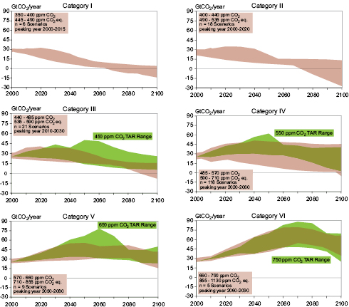
Figure 3.17: Emissions pathways of mitigation scenarios for alternative groups of stabilization targets (Categories I to VI, see Table 3.5). The pink area gives the projected CO2 emissions for the recent mitigation scenarios developed post-TAR. Green shaded areas depict the range of more than 80 TAR stabilization scenarios ( Morita et al., 2001 [NPR, SRC] ). Category I and II scenarios explore stabilization targets below the lowest target of the TAR.
The emission range for the scenarios with low and intermediate targets between 3.5 and 5 W/m2 (scenarios in categories III and IV) are consistent with the range of the 450 and 550 ppmv CO2 scenarios in the TAR. Emissions in this category tend to show peak emissions around 2040 – with emissions in 2100 similar to, or slightly below, emissions today. Although for these categories less rapid and forceful reductions are required than for the more stringent targets, studies focusing on these stabilization categories find that a wide portfolio of reduction measures would be needed to achieve such emission pathways in a cost-effective way.
The two highest categories of stabilization scenarios (V and VI) overlap with low-medium category baseline scenarios (see Section 3.2 ). This partly explains the relatively small number of new studies on these categories. The emission profiles of these scenarios are found to be consistent with the emissions ranges as published in the TAR.
There is a relatively strong relationship between the cumulative CO2 emissions in the 2000 – 2100 period and the stringency of climate targets (see Figure 3.18 ). The uncertainties associated with individual stabilization levels (shown by the different percentiles [9] ) are primarily due to the ranges associated with individual stabilization categories, substitutability of CO2 and non-CO2-emissions, different model parameterizations of the carbon cycle, but they are also partly due to differences in emissions pathways (delayed reduction pathways can allow for somewhat higher cumulative emissions). In general, scenarios aiming for targets below 3 W/m2 require cumulative CO2 emissions of around 1100 GtCO2 (range of 800– 1500 GtCO2). The cumulative emissions increase for subsequently less stringent targets. The middle category (4–5 W/m2) requires emissions to be in the order of 3000 GtCO2 (range of 2270 –3920 GtCO2). The highest category (>6 W/m2) exhibits emissions, on average, around 5020 GtCO2 (range of 4400–6600 GtCO2).
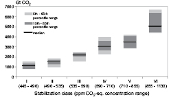
Figure 3.18: Relationship between the scenario’s cumulative carbon dioxide emissions ( 2000 – 2100 ) and the stabilization target (stabilization categories I to VI, of Table 3.5).
The timing of emission reductions also depends on the stringency of the stabilization target. Timing of climate policy has always been an important topic in the scenario literature. While some studies argue for early action for smooth transitions and stimulating technology development (e.g. ( Azar and Dowlatabadi, 1999, ) van Vuuren and de Vries, 2001 [JoC, SRC] ), others emphasize delayed response to benefit from better technology and higher CO2 fertilization rates from natural systems at later points in time (e.g. Wigley et al., 1996 [JoC, SRC] ;( Tol, 2000; ) for a more elaborate discussion on timing see also Section 3.6 ). This implies that a given stabilization target can be consistent with a range of interim targets. Nevertheless, stringent targets require an earlier peak of CO2 emissions (see Figure 3.19 and Table 3.5 ). In the majority of the scenarios concerning the most stringent group (< 3 W/m2), emissions start to decline before 2015, and are further reduced to less than 50% of today’s emissions by 2050 ( Table 3.5 ). The emissions profiles of these scenarios indicate the need for short-term infrastructure investments for a comparatively early decarbonization of the energy system. Achieving these low-emission trajectories requires a comprehensive global mitigation effort, including a further tightening of existing climate policies in Annex I countries, and simultaneous emission mitigation in developing countries, where most of the increase in emissions is expected in the coming decades. For the medium stringency group (4-5 W/m2) the peak of global emissions generally occurs around 2010 to 2030; followed by a return to 2000 levels, on average, around 2040 (with the majority of these scenarios returning to 2000 emissions levels between 2020 and 2060 ). For targets between 5–6 W/m2, the median emissions peak around 2070 . The figure also indicates that the uncertainty range is relatively small for the more stringent targets, illustrating the reduced flexibility of the emissions path and the requirement for early mitigation. The less stringent categories allow more flexibility in timing. Most of the stringent stabilization scenarios of category I (and some II scenarios) assume a temporal overshoot of the stabilization target (GHG concentration, radiative forcing, or temperature change) before the eventual date of stabilization between 2100 and 2150 . Recent studies indicate that while such ‘overshoot’ strategies might be inevitable for very low targets (given the climate system and socio-economic inertia), they might also provide important economic benefits. At the same time, however, studies note that the associated rate of warming from large overshoots might significantly increase the risk of exceeding critical climate thresholds. (For further discussion, see Section 3.3.4 .)
The right-hand panel of Figure 3.19 illustrates the time at which CO2 emissions will have to return to present levels. For stringent stabilization targets (below 4 W/m2; category I, II and III) emissions return to present levels, on average, before the middle of this century, that is about one to two decades after the year in which emissions peak. In most of the scenarios for the highest stabilization category (above 6 W/m2; category VI) emissions could stay above present levels throughout the century.
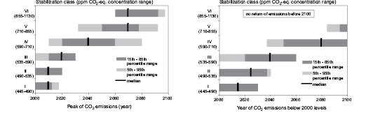
Figure 3.19: Relationship between the stringency of the stabilization target (category I to VI) and 1) the time at which CO2 emissions have to peak (left-hand panel), and 2) the year when emissions return to present ( 2000 ) levels.
The absolute level of the required emissions reduction does not only depend on the stabilization target, but also on the baseline emissions (see Hourcade and Shukla, 2001 [NPR, ARC] ). This is clearly shown in the right-hand panel of Figure 3.20 , which illustrates the relationship between the cumulative baseline emissions and the cumulative emissions reductions for the stabilization scenarios (by 2100 ). In general, scenarios with high baseline emissions require a higher reduction rate to reach the same reduction target: this implies that the different reduction categories need to show up as diagonals in figure 3.20 . This is indeed the case for the range of studies and the ‘category averages’ (large triangles). As indicated in the figure, a scenario with high baseline emissions requires much deeper emission reduction in order to reach a medium stabilization target (sometimes more than 3600 GtCO2) than a scenario with low baseline emissions to reach the most stringent targets (in some cases less than 1800 GtCO2). For the same target (e.g. category IV) reduction may differ from 370 to 5500 GtCO2. This comes from the large spread of emissions in the baseline scenarios. While scenarios for both stringent and less-stringent targets have been developed from low and high baseline scenarios, the data suggests that, on average, mitigation scenarios aimed at the most stringent targets start from the lowest baseline scenarios.
In the short-term ( 2030 ), the relationship between emission reduction and baseline is less clear, given the flexibility in the timing of emission reductions (left-hand panel in Figure 3.20 ). While the averages of the various stabilization categories are aligned in a similar way to those discussed for 2100 (with exception of category I, for which the scenario sample is smaller than for the other categories); the uncertainty ranges here are very large.

3.3.5.2 GHG abatement measures
The abatement of GHG emissions can be achieved through a wide portfolio of measures in the energy, industry, agricultural and forest sectors (see also Edmonds et al., 2004b [MoS, ARC] ; Pacala and Socolow, 2004 [JoC] ; Metz and van Vuuren, 2006 [NPR, SRC] ). Measures for reducing CO2 emissions range from structural changes in the energy system and replacement of carbon-intensive fossil fuels by cleaner alternatives (such as a switch from coal to natural gas, or the enhanced use of nuclear and renewable energy), to demand-side measures geared towards energy conservation and efficiency improvements. In addition, capturing carbon during energy conversion processes with subsequent storage in geological formations (CCS) provides an approach for reducing emissions. Another important option for CO2 emission reduction encompasses the enhancement of forest sinks through afforestation, reforestation activities and avoided deforestation.
In the energy sector the aforementioned options can be grouped into two principal measures for achieving CO2 reductions:
1. Improving the efficiency of energy use (or measures geared towards energy conservation).
2. Reducing the emissions per unit of energy consumption.
The latter comprises the aggregated effect of structural changes in the energy systems and the application of CCS. A response index has been calculated (based on the full set of stabilization scenarios from the database) in order to explore the importance of these two strategies. This index is equal to the ratio of the reductions achieved through energy efficiency over those achieved by carbon-intensity improvements ( Figure 3.21 ). Similar to Morita et al. 2001 [NPR, SRC] ), it was discovered that the mitigation response to reduce CO2 emissions would shift over time, from initially focusing on energy efficiency reductions in the beginning of the 21st century to more carbon-intensity reduction in the latter half of the century ( Figure 3.21 ). The amount of reductions coming from carbon-intensity improvement is more important for the most stringent scenarios. The main reason is that, in the second half of the century, increasing costs of further energy efficiency improvements and decreasing costs of low-carbon or carbon-free energy sources make the latter category relatively more attractive. This trend is also visible in the scenario results of model comparison studies ( Weyant, 2004 [SRC] ; Edenhofer et al., 2006 [NPR, ARC] ).
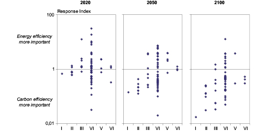
Figure 3.21: Response index to assess priority setting in energy-intensity reduction (more than 1) or in carbon-intensity reduction (less than 1) for post-TAR stabilization scenarios.
In addition to measures for reducing CO2 emissions from energy and industry, emission reductions can also be achieved from other gases and sources. Figure 3.22 illustrates the relative contribution of measures towards achieving climate stabilization from three main sources:
1. CO2 from energy and industry.
2. CO2 from land-use change.
3. The full basket of non-CO2 emissions from all relevant sources.
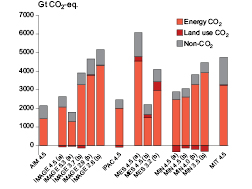
The figure compares the contribution of these measures towards achieving stabilization for a wide range of targets (between 2.6 and 5.3 W/m2 by 2100 ) and baseline scenarios. An important conclusion across all stabilization levels and baseline scenarios is the central role of emissions reductions in the energy and industry sectors. All stabilization studies are consistent in that (independent of the baseline or target uncertainty) more than 65% of total emissions reduction would occur in this sector. The non-CO2 gases and land-use-related CO2 emissions (including forests) are seen to contribute together up to 35% of total emissions reductions. [10] However, as noted further above, the majority of recent studies indicate the relative importance of the latter two sectors for the cost-effectiveness of integrated multi-gas GHG abatement strategies (see also Section 3.3.5.4 on CO2-only versus multi-gas mitigation and 3.3.5.5 on land-use).
The strongest divergence across the scenarios concerns the contribution of land-use-related mitigation. The results range from negative contributions of land-use change to potential emissions savings of more than 1100 GtCO2 over the course of the century ( Figure 3.22 ). The primary reason for this is the considerable uncertainty with respect to future competition for land between dedicated bio-energy plantations and potential gains from carbon savings in terrestrial sinks. Some scenarios, for example, project massive expansion of dedicated bio-energy plantations, leading to an increase in emissions due to net deforestation (compared to the baseline).
An illustrative example for the further breakdown of mitigation options is shown in Figure 3.23 . The figure shows stabilization scenarios for a range of targets (about 3–4.5 W/m2) based on four illustrative models (IMAGE, MESSAGE, AIM and IPAC) for which sufficient data were available. The scenarios share similar stabilization targets, but differ with respect to salient assumptions for technological change, long-term abatement potentials, as well as model methodology and structure. The scenarios are also based on different baseline scenarios. For example, cumulative baseline emissions over the course of the century range between 6000 GtCO2-eq in MESSAGE and IPAC scenarios to more than 7000 GtCO2-eq in the IMAGE and AIM scenarios. Figure 3.24 shows the primary energy mix of the baseline and the mitigation scenarios.
It should be noted that the figure shows reduction on top of the baseline (e.g. other renewables may already make a large baseline contribution). Above all, Figure 3.23 illustrates the importance of using a wide portfolio of reduction measures, with many categories of measures, showing contributions of more than a few hundred GtCO2 over the course of the century. In terms of the contribution of different options, there is agreement for some options, while there is disagreement for others. The category types that have a large potential over the long term ( 2000 – 2100 ) in at least one model include energy conservation, carbon capture and storage, renewables, nuclear and non-CO2 gases. These options could thus constitute an important part of the mitigation portfolio. However, the differences between the models also emphasize the impact of different assumptions and the associated uncertainty (e.g. for renewables, results can vary strongly depending on whether they are already used in the baseline, and how this category competes against other zero or low-emission options in the power sector, such as nuclear and CCS). The figure also illustrates that the limitations of the mitigation portfolio with respect to CCS or forest sinks (AIM and IPAC) would lead to relatively higher contributions of other options, in particular nuclear (IPAC) and renewables (AIM).
Figure 3.23 also illustrates the increase in emissions reductions necessary to strengthen the target from 4.5 to about 3–3.6 W/m2. Most of the mitigation options increase their contribution significantly by up to a factor of more than two. This effect is particularly strong over the short term ( 2000 – 2030 ), indicating the need for early abatement in meeting stringent stabilization targets. Another important conclusion from the figure is that CCS and forest sink options are playing a relatively modest role in the short-term mitigation portfolio, particularly for the intermediate stabilization target (4.5 W/m2). The results thus indicate that the widespread deployment of these options might require relatively more time compared to the other options and also relatively higher carbon prices (see also Figure 3.25 on increasing carbon prices over time).
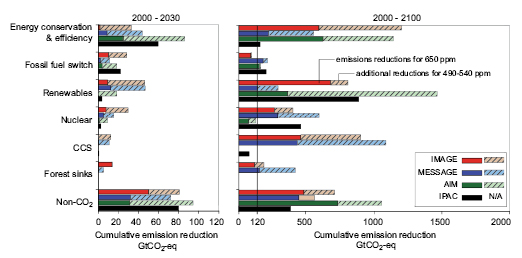
Figure 3.23: Cumulative emissions reductions for alternative mitigation measures for 2000 to 2030 (left-hand panel) and for 2000 - 2100 (right-hand panel). The figure shows illustrative scenarios from four models (AIM, IMAGE, IPAC and MESSAGE) for stabilization levels of 490-540 ppmv CO2-eq and levels of 650 ppmv CO2-eq, respectively. Dark bars denote reductions for a target of 650 ppmv CO2-eq and light bars the additional reductions to achieve 490-540 ppmv CO2-eq. Note that some models do not consider mitigation through forest sink enhancement (AIM and IPAC) or CCS (AIM) and that the share of low-carbon energy options in total energy supply is also determined by inclusion of these options in the baseline. CCS includes carbon capture and storage from biomass. Forest sinks include reducing emissions from deforestation.
As noted above, assumptions with regards to the baseline can have significant implications for the contribution of individual mitigation options in achieving stabilization. Figure 3.24 clearly shows that the baseline assumptions of the four models differ, and that these differences play a role in explaining some of the results. For instance, the MESSAGE model already includes a large amount of renewables in its baseline and further expansion is relatively costly. Nevertheless, some common trends among the models may also be observed. First of all, almost all cases show a clear reduction in primary energy use. Second, in all models coal use is significantly reduced under the climate policy scenarios, compared to the baseline. It should be noted that in those models that consider CCS, the remaining fossil fuel use is mostly in combination with carbon capture and storage. In 2030, oil use is only modestly reduced by climate policies – this also applies to natural gas use. In 2100, both oil and gas are reduced compared to the baseline in most models. Finally, renewable energy and nuclear power increase in all models – although the distribution across these two options differs.
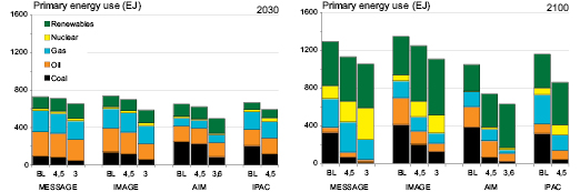
3.3.5.3 Stabilization costs
Models use different metrics to report the costs of emission reductions. Top-down general equilibrium models tend to report GDP losses, while system-engineering partial equilibrium models usually report the increase in energy system costs or the net present value (NPV) of the abatement costs. A common cost indicator is also the marginal cost/price of emissions reduction (US$/tC or US$/tCO2).
Figure 3.25 shows the relationship between stabilization targets and alternative measures of mitigation costs, comprising GDP losses, net present value of abatement, and carbon price in terms of US$ /tCO2-eq.
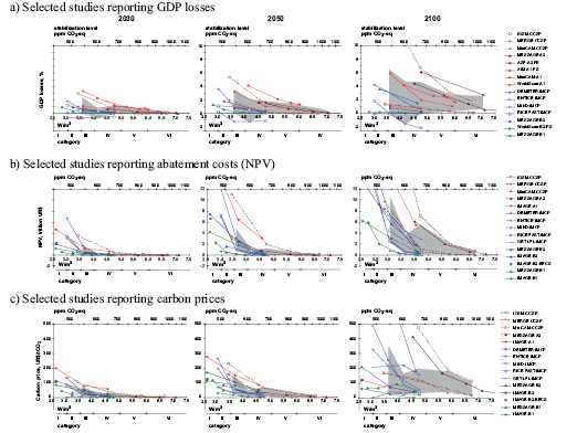
Figure 3.25: Relationship between the cost of mitigation and long-term stabilization targets (radiative forcing compared to pre-industrial level, W/m2 and CO2-eq concentrations).
It is important to note that for the following reported cost estimates, the vast majority of the models assume transparent markets, no transaction costs, and thus perfect implementation of policy measures throughout the 21st century, leading to the universal adoption of cost-effective mitigation measures, such as carbon taxes or universal cap and trade programmes. These assumptions generally result in equal carbon prices across all regions and countries equivalent to global, least-cost estimates. Relaxation of these modelling assumptions, alone or in combination (e.g. mitigation-only in Annex I countries, no emissions trading, or CO2-only mitigation), will lead to an appreciable increase in all cost categories.
The grey shaded area in Figure 3.25 illustrates the 10th–90th percentile of the mitigation cost ranges of recent studies, including the TAR. The area includes only those recent scenarios in the literature that report cost estimates based on a comprehensive mitigation analysis, defined as those that have a sufficiently wide portfolio of mitigation measures. [11] The selection was made on a case-by-case basis for each scenario considered in this assessment. The Figure also shows results from selected illustrative studies (coloured lines). These studies report costs for a range of stabilization targets and are representative of the overall cost dynamics of the full set of scenarios. They show cases with high-, intermediate- and low-cost estimates (sometimes exceeding the 80th (i.e. 10th–90th) percentile range on the upper and lower boundaries of the grey-shaded area). The colour coding is used to distinguish between individual mitigation studies that are based on similar baseline assumptions. Generally, mitigation costs (for comparable stabilization targets) are higher from baseline scenarios with relatively high baseline emissions (brown and red lines). By the same token, intermediate or low baseline assumptions result in relatively lower cost estimates (blue and green lines).
Figure 3.25 a shows that the majority of studies find that GDP losses increase with the stringency of the target, even though there is considerable uncertainty with respect to the range of losses. Barker et al. 2006 [NPR, SRC] ) found that, after allowing for baseline emissions, the differences can be explained by:
- The spread of assumptions in modelling-induced technical change.
- The use of revenues from taxes and permit auctions.
- The use of flexibility mechanisms (i.e. emissions trading, multi-gas mitigation, and banking).
- The use of backstop technologies.
- Allowing for climate policy related co-benefits.
- Other specific modelling assumptions.
Weyant 2000 [NPR, SRC] ) lists similar factors but also includes the number and type of technologies covered, and the possible substitution between cost factors (elasticities). A limited set of studies finds negative GDP losses (economic gains) that arise from the assumption that a model’s baseline is assumed to be a non-optimal pathway and incorporates market imperfections. In these models, climate policies steer economies in the direction of reducing these imperfections, for example by promoting more investment into research and development and thus achieving higher productivity, promoting higher employment rates, or removing distortionary taxes.
The left-hand side panel of Figure 3.25 a shows that for 2030, GDP losses in the vast majority of the studies (more than 90% of the scenarios) are generally below 1% for the target categories V and VI. Also in the majority of the category III and IV scenarios (70% of the scenarios) GDP losses are below 1%. However, it is important to note that for categories III and IV costs are higher, on average, and show a wider range than those for categories V and VI. For instance, for category IV the interval lying between the 10th and 90th percentile varies from about 0.6% gain to about 1.2% loss. For category III, this range is shifted upwards (0.2–2.5%). This is also indicated by the median GDP losses by 2030, which increases from below 0.2% for categories V and VI, to about 0.2% for the category IV scenarios, and to about 0.6% for category III scenarios. GDP losses of the lowest stabilization categories (I & II) are generally below 3% by 2030, however the number of studies are relatively limited and in these scenarios stabilization is achieved predominantly from low baselines. The absolute GDP losses by 2030 correspond on average to a reduction of the annual GDP growth rate of less than 0.06 percentage points for the scenarios of category IV, and less than 0.1 and 0.12 percentage points for the categories III and I&II, respectively.
GDP losses by 2050 (middle panel of Figure 3.25 a) are comparatively higher than the estimates for 2030 . For example, for category IV scenarios the range is between -1% and 2% GDP loss compared to baseline (median 0.5%), and for category III scenarios the range is from slightly negative to 4% (median 1.3%). The Stern review ( 2006 ), looking at the costs of stabilization in 2050 for a comparable category (500–550 CO2-eq) found a similar range of between -2% and +5%. For the studies that also explore different baselines (in addition to multiple stabilization levels), Figure 3.25 a also shows that high emission baselines (e.g. high SRES-A1 or A2 baselines) tend to lead to higher costs. However, the uncertainty range across the models is at least of a similar magnitude. Generally, models that combine assumptions of very slow or incremental technological change with high baseline emissions (e.g. IGSM-CCSP) tend to show the relatively highest costs ( Figure 3.25 a). GDP losses of the lowest stabilization categories (I & II) are generally below 5.5% by 2050, however the number of studies are relatively limited and in these scenarios stabilization is achieved predominantly from low baselines. The absolute GDP losses numbers for 2050 reported above correspond on average to a reduction of the annual GDP growth rate of less than 0.05 percentage points for the scenarios of category IV, and less than 0.1 and 0.12 percentage points for the categories III and I&II, respectively.
Finally, the most right-hand side panel of Figure 3.25 a shows that GDP losses show a bigger spread and tend to be somewhat higher by 2100 . GDP losses are between 0.3% and 3% for category V scenarios and -1.6% to about 5% for category IV scenarios. Highest costs are given by category III (from slightly negative costs up to 6.5%). The sample size for category I is not large enough for a statistical analysis. Similarly, for category II scenarios, the range is not shown as the stabilization scenarios of category II are predominantly based on low or intermediate baselines, and thus the resulting range would not be comparable to those from the other stabilization categories. However, individual studies indicate that costs become higher for more stringent targets (see, for example, studies highlighted in green and blue for the lowest stabilization categories in Figure 3.25 a). [12]
The results for the net present value of cumulative abatement costs show a similar picture ( Figure 3.25 b). However, given the fact that abatement costs only capture direct costs, this cost estimate is by definition more certain. [13] The interval from the 10th to the 90th percentile in 2100 ranges from nearly zero to about 11 trillion US$. The highest level corresponds to around 2–3% of the NPV of global GDP over the same period. Again, on the basis of comparison across models, it is clear that costs depend both on the stabilization level and baseline emissions. In general, the spread of costs for each stabilization category seems to be of a similar order to the differences across stabilization scenarios from different baselines. In 2030, the interval covering 80% of the NPV estimates runs from around 0–0.3 trillion for category IV scenarios. The majority of the more stringent (category III) scenarios range between 0.2 to about 1.6 trillion US$. In 2050, typical numbers for category IV are around 0.1–1.2 trillion US$ and, for category III, this is 1–5 trillion US$ (or below about 1% of the NPV of GDP). By 2100 the NPV estimates increase further, with the range up to 5 trillion for category IV scenarios and up to 11 trillion for category III scenarios, respectively. The results of these studies, published since the TAR, are consistent with the numbers presented in the TAR, although the new studies extend results to substantially lower stabilization levels.
Finally, a similar trend is found for carbon price estimates. In 2030, typical carbon prices across the range of models and baselines for a 4.5 W/m2 stabilization target (category IV) range from around 1–24 US$/tCO2 (80% of estimates), with the median of about 11 US$/tCO2. For category III, the corresponding prices are somewhat higher and range from 18–79 US$/tCO2 (with the median of the scenarios around 45 US$/tCO2). Most individual studies for the most stringent category cluster around prices of about 100 US$/tCO2. [14] Carbon prices by 2050 are comparatively higher than those in 2030 . For example, costs of category IV scenarios by 2050 range between 5 and 65 US$/tCO2, and those for category III range between 30 and 155 US$/tCO2. Carbon prices in 2100 vary over a much wider range – mostly reflecting uncertainty in baseline emissions and technology development. For the medium target of 4.5 W/m2, typical carbon prices in 2100 range from 25–200 US$/tCO2 (80% of estimates). This is primarily a consequence of the nature of this metric, which often represents costs at the margin. Costs tend to slowly increase for more stringent targets – with a range between the 10th and 90th percentile of more than 35 to about 350 US$/tCO2 for category III.
3.3.5.4 The role of non-CO2 GHGs
As also illustrated by the scenario assessment in the previous sections, more and more attention has been paid since the TAR to incorporating non-CO2 gases into climate mitigation and stabilization analyses. As a result, there is now a body of literature (e.g. van Vuuren et al., 2006b [MoS, SRC] ; de la Chesnaye and Weyant, 2006 [SRC] ; de la Chesnaye et al., 2007 [NPR, MoS, SRC, 2007] ) showing that mitigation costs for these sectors can be lower than for energy-related CO2 sectors. As a result, when all these options are employed in a multi-gas mitigation policy, there is a significant potential for reduced costs, for a given climate policy objective, versus the same policy when CO2 is the only GHG directly mitigated. These cost savings can be especially important where carbon dioxide is not the dominant gas, on a percentage basis, for a particular economic sector and even for a particular region. While the previous sections have focused on the joint assessment of CO2 and multi-gas mitigation scenarios, this section explores the specific role of non-CO2 emitting sectors. [15]
A number of parallel numerical experiments have been carried out by the Energy Modelling Forum (EMF-21; de la Chesnaye and Weyant, 2006 [SRC] ). The overall conclusion is that economic benefits of multi-gas strategies are robust across all models. This is even true, despite the fact that different methods were used in the study to compare the relative contribution of these gases in climate forcing (see Section 3.3.3 ). The EMF-21 study specifically focused on comparing stabilization scenarios aiming for 4.5 W/m2 compared to pre-industrial levels. There were two cases employed to achieve the mitigation target:
1. Directly mitigate CO2 emissions from the energy sector (with some indirect reduction in non-CO2 gases).
2. Mitigate all available GHG in costs-effective approaches using full ‘what’ flexibility.
In the CO2-only mitigation scenario, all models significantly reduced CO2 emissions, on average by about 75% in 2100 compared to baseline scenarios. Models still indicated some emission reductions for CH4 and N2O as a result of systemic changes in the energy system. Emissions of CH4 were reduced by about 20% and N2O by about 10% ( Figure 3.26 ).
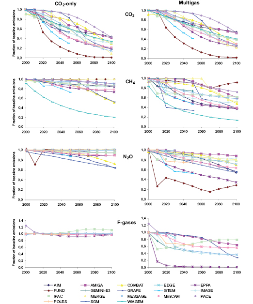
In the multi-gas mitigation scenario, all models found that an appreciable percentage of the emission reductions occur through reductions of non-CO2 gases, which then results in smaller required reductions of CO2. The emission reduction for CO2 in 2100 therefore drops (on average) from 75% to 67%. This percentage is still rather high, caused by the large share of CO2 in total emissions (on average, 60% in 2100 ) and partly due to the exhaustion of reduction options for non-CO2 gases. The reductions of CH4 across the different models averages around 50%, with remaining emissions coming from sources for which no reduction options were identified, such as CH4 emissions from enteric fermentation. For N2O, the increased reduction in the multi-gas strategy is not as large as for CH4 (almost 40%). The main reason is that the identified potential for emission reductions for the main sources of N2O emissions, fertilizer use and animal manure, is still limited. Finally, for the fluorinated gases, high reduction rates (about 75%) are found across the different models.
Although the contributions of different gases change sharply over time, there is a considerable spread among the different models. Many models project relatively early reductions of both CH4 and the fluorinated gases under the multi-gas case. However, the subset of models that does not use GWPs as the substitution metric for the relative contributions of the different gases to the overall target, but does assume inter-temporal optimization in minimizing abatement costs, do not start to reduce CH4 emissions substantially until the end of the period. The increased flexibility of a multi-gas mitigation strategy is seen to have significant implications for the costs of stabilization across all models participating in the EMF-21. These scenarios concur that multi-gas mitigation is significantly cheaper than CO2-only. The potential reductions of the GHG price ranges in the majority of the studies between 30% and 85% (See Figure 3.27 ).
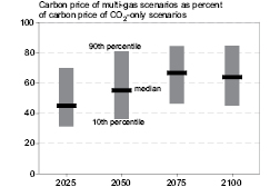
Figure 3.27: Reduction in GHG abatement price (%) in multi-gas stabilization scenarios compared to CO2-only cases. Ranges correspond to alternative scenarios for a stabilization target of 4.5 W/m2.
Finally, the EMF-21 research also showed that, for some sources of non-CO2 gases, the identified reduction potential is still very limited (e.g. most agricultural sources for N2O emissions). For long-term scenarios (and more stringent targets) in particular, identifying how this potential may develop in time is a crucial research question. Attempts to estimate the maximum feasible reductions (and the development of potential over time) have been made in van Vuuren et al. 2007 [JoC, SRC, 2007] ).
3.3.5.5 Land use
Changes in land-use practices are regarded as an important component of long-term strategies to mitigate climate change. Modifications to land-use activities can reduce emissions of both CO2 and non-CO2 gases (CH4 and N2O), increase sequestration of atmospheric CO2 into plant biomass and soils, and produce biomass fuel substitutes for fossil fuels (see Chapters 4 , 8 , and 9 of this report for discussions of detailed land-related mitigation alternatives). Available information before the TAR suggested that land has the technical potential to sequester up to an additional 319 billion tonnes of CO2 (GtCO2) by 2050 in global forests alone ( IPCC, 1996a [NPR] ; IPCC, 2000 [NPR] ; IPCC, 2001a [NPR] ). In addition, current technologies are capable of substantially reducing CH4 and N2O emissions from agriculture (see Chapter 8 ). A number of global biomass energy potential assessments have also been conducted (see Berndes et al. 2003 [MoS, ARC] for an overview). [16]
The explicit modelling of land-based climate change mitigation in long-term global scenarios is relatively new and rapidly developing. As a result, assessment of the long-term role of global land-based mitigation was not formally addressed by the Special Report on Land use, Land-use Change, and Forestry ( IPCC, 2000 [NPR] ) or the TAR. This section assesses the modelling of land in long-term climate stabilization and the relationship to detailed global forestry mitigation estimates from partial equilibrium sectoral models that model 100-year carbon price trajectories.
Development of, among other things, global sectoral land mitigation models (e.g. Sohngen and Sedjo, 2006 [NPR, ARC] ), bottom-up agricultural mitigation costs for specific technologies (e.g. USEPA, 2006b [NPR] ), and biomass technical potential studies (e.g. Hoogwijk et al., 2005 [SRC] ) has facilitated the formal incorpo-ration of land mitigation in long-term integrated assessment of climate change stabilization strategies. Hoogwijk et al. 2005 [SRC] ), for example, estimated the potential of abandoned agricultural lands for providing biomass for primary energy demand and identified the technical biomass supply limits of this land type (e.g. under the SRES A2 scenario, abandoned agricultural lands could provide for 20% of 2001 total energy demand). Sands and Leimbach 2003 [JoC, MoS] ) conducted one of the first studies to explicitly explore land-based mitigation in stabilization, suggesting that the total cost of stabilization could be reduced by including land strategies in the set of eligible mitigation options (energy crops in this case). The Energy Modelling Forum Study-21 (EMF-21; de la Chesnaye and Weyant, 2006 [SRC] ) was the first coordinated stabilization modelling effort to include an explicit evaluation of the relative role of land in stabilization; however, only a few models participated. Building on their EMF-21 efforts, some modelling teams have also generated even more recent stabilization scenarios with revised land modelling. These studies are conspicuously different in the specifics of their modelling of land and land-based mitigation ( Rose et al., 2007 [NPR, MoS, SRC, 2007] ). Differences in the types of land considered, emissions sources, and mitigation alternatives and implementation imply different opportunities and opportunity costs for land-related mitigation; and, therefore, different outcomes.
Four of the modelling teams in the EMF-21 study directly explored the question of the cost-effectiveness of including land-based mitigation in stabilization solutions and found that including these options (both non-CO2 and CO2) provided greater flexibility and was cost-effective for stabilizing radiative forcing at 4.5 W/m2 ( Kurosawa, 2006 [NPR] ; van Vuuren et al., 2006a [NPR, MoS, SRC] ; Rao and Riahi, 2006 [SRC] ; Jakeman and Fisher, 2006 [NPR, SRC] Jakeman and Fisher 2006 [NPR, SRC] ), for example, found that including land-use change and forestry mitigation options reduced the emissions reduction burden on all other emissions sources such that the projected decline in global real GDP associated with achieving stabilization was reduced to 2.3% at 2050 (3.4 trillion US$), versus losses of around 7.1% (10.6 trillion US$) and 3.3% (4.9 trillion US$) for the CO2-only and multi-gas scenarios, respectively. [17] Unfortunately, none of the EMF-21 papers isolated the GDP effects associated with biomass fuel substitution or agricultural non-CO2 abatement. However, given agriculture’s small estimated share of total abatement (discussed below), the GDP savings associated with agricultural non-CO2 abatement could be expected to be modest overall, though potentially strategically significant to the dynamics of mitigation portfolios. Biomass, on the other hand, may have a substantial abatement role and therefore a large effect on the economic cost of stabilization. Notably, strategies for increasing cropland soil carbon have not been incorporated to date into this class of models (see Chapter 8 for an estimate of the short-term potential for enhancing agricultural soil carbon).
Figure 3.28 presents the projected mitigation from forestry, agriculture, and biomass for the EMF-21 4.5 W/m2 stabilization scenarios, as well as additional scenarios produced by the MESSAGE and IMAGE models – an approximate 3 W/m2 scenario from Rao and Riahi 2006 [SRC] ), a 4.5 W/m2 scenario from Riahi et al. 2006 [NPR, SRC] ), and approximately 4.5, 3.7, and 2.9 W/m2 scenarios from van Vuuren et al. 2007 [JoC, SRC, 2007] ) (see Rose et al., 2007 [NPR, MoS, SRC, 2007] , for a synthesis). While there are clearly different land-based mitigation pathways being taken across models for the same stabilization target, and across targets with the same model and assumptions, some general observations can be made. First, forestry, agriculture, and biomass are called upon to provide significant cost-effective mitigation contributions ( Rose et al., 2007 [NPR, MoS, SRC, 2007] ). In the short-term ( 2000 – 2030 ), forest, agriculture, and biomass together could account for cumulative abatement of 10–65 GtCO2-eq, with 15–60% of the total abatement considered by the available studies, and forest/agricultural non-CO2 abatement providing at least three quarters of total land abatement. [18] Over the entire century ( 2000 – 2100 ), cumulative land-based abatement of approximately 345– 1260 GtCO2-eq is estimated to be cost-effective, accounting for 15–40% of total cumulative abatement. Forestry, agriculture, and biomass abatement levels are each projected to grow annually with relatively stable annual increases in agricultural mitigation and gradual deployment of biomass mitigation, which accelerates dramatically in the last half of the century to become the dominant land-mitigation strategy.
Figures 3.28 and 3.29 show that additional land-based abatement is expected to be cost-effective with tighter stabilization targets and/or higher baseline emissions (e.g. see the IMAGE 2.3 results for various stabilization targets and the MESSAGE 4.5 W/m2 stabilization results with B2 (EMF-21) and A2r baselines). Biomass is largely responsible for the additional abatement; however, agricultural and forestry abatement are also expected to increase. How they might increase is model and time dependent. In general, the overall mitigation role of agricultural abatement of rice methane, livestock methane, nitrous oxide (enteric and manure) and soil nitrous oxide is projected to be modest throughout the time horizon, with some suggestion of increased importance in early decades.
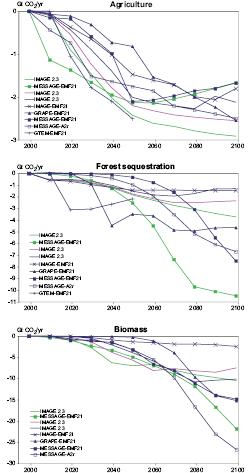
Figure 3.28: Cost-effective agriculture, forest, and commercial biomass annual greenhouse gas emissions abatement from baselines from various 2100 stabilization scenarios (note y-axes have different ranges).
However, there are substantial uncertainties. There is little agreement about the magnitudes of abatement (Figures 3.28 and 3.29 ). The scenarios disagree about the role of agricultural strategies targeting CH4 versus N2O, as well as the timing and annual growth of forestry abatement, with some scenarios suggesting substantial early deployment of forest abatement, while others suggest gradual annual growth or increasing annual growth.
A number of the recent scenarios suggest that biomass energy alternatives could be essential for stabilization, especially as a mitigation strategy that combines the terrestrial sequestration mitigation benefits associated with bio-energy CO2 capture and storage (BECCS), where CO2 emissions are captured during biomass energy combustion for storage in geologic formations (e.g. Rao and Riahi, 2006 [SRC] ; Riahi et al., 2006 [NPR, SRC] ; Kurosawa, 2006 [NPR] ; van Vuuren et al., 2007 [JoC, SRC, 2007] ; USCCSP, 2006 [NPR] ). BECCS has also been suggested as a potential rapid-response prevention strategy for abrupt climate change. Across stabilization scenarios, absolute emissions reductions from biomass are projected to grow slowly in the first half of the century, and then rapidly in the second half, as new biomass processing and mitigation technologies become available. Figure 3.28 suggests biomass mitigation of up to 7 GtCO2/yr in 2050 and 27 GtCO2/yr in 2100, for cumulative abatement over the century of 115–749 GtCO2 ( Figure 3.29 ). Figure 3.30 shows the amount of commercial biomass primary energy utilized in various stabilization scenarios. For example, in 2050, the additional biomass energy provides approximately 5–55 EJ for a 2100 stabilization target of 4–5 W/m2 and approximately 40–115 EJ for 3.25–4 W/m2, accounting for about 0–10 and 5–20% of 2050 total primary energy respectively ( USCCSP, 2006 [NPR] ; Rose et al., 2007 [NPR, MoS, SRC, 2007] ). Over the century, the additional bio-energy accounts for 500–6,700 EJ for targets of 4–5 W/m2 and 6100–8000 EJ for targets of 3.25–4 W/m2 (1–9% and 9–13% of total primary energy, respectively).
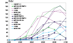
Figure 3.30: Commercial biomass primary energy scenarios above baseline from various 2100 stabilization scenarios.
More biomass energy is supplied with tighter stabilization targets, but how much is required for any particular target depends on the confluence of the many different modelling assumptions. Modelled demands for biomass include electric power and end-use sectors (transportation, buildings, industry, and non-energy uses). Current scenarios suggest that electric power is projected to dominate biomass demand in the initial decades and, in general, with less stringent stabilization targets. Later in the century (and for more stringent targets) transportation is projected to dominate biomass use. When biomass is combined with BECCS, biomass mitigation shifts to the power sector late in the century, to take advantage of the net negative emissions from the combined abatement option, such that BECCS could represent a signifant share of cumulative biomass abatement over the century (e.g. 30–50% of total biomass abatement from MESSAGE in Figure 3.29 ).
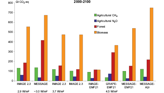
Figure 3.29: Cumulative cost-effective agricultural, forestry, and biomass abatement 2000 – 2100 from various 2100 stabilization scenarios.
To date, detailed analyses of large-scale biomass conversion with CO2 capture and storage is scarce. As a result, current integrated assessment BECCS scenarios are based on a limited and uncertain understanding of the technology. In general, further research is necessary to characterize biomass’ long-term mitigation potential, especially in terms of land area and water requirements, constraints, and opportunity costs, infrastructure possibilities, cost estimates (collection, transportation, and processing), conversion and end-use technologies, and ecosystem externalities. In particular, present studies are relatively poor in representing land competition with food supply and timber production, which has a significant influence on the economic potential of bio-energy crops (an exception is Sands and Leimbach, 2003 [JoC, MoS] ).
Terrestrial mitigation projections are expected to be regionally unique, while still linked across time and space by changes in global physical and economic forces. For example, Rao and Riahi 2006 [SRC] ) offer intuitive results on the potential role of agricultural methane and nitrous oxide mitigation across industrialized and developing country groups, finding that agriculture is expected to form a larger share of the developing countries’ total mitigation portfolio; and, developing countries are likely to provide the vast majority of global agricultural mitigation. Some aggregate regional forest mitigation results also are discussed below. However, given the paucity of published regional results from integrated assessment models, it is currently not possible to assess the regional land-use abatement potential in stabilization. Future research should direct attention to this issue in order to more fully characterize mitigation potential.
In addition to the stabilization scenarios discussed thus far from integrated assessment and climate economic models, the literature includes long-term mitigation scenarios from global land sector economic models (e.g. Sohngen and Sedjo, 2006 [NPR, ARC] ; Sathaye et al., 2006 [NPR, ARC] ; Sands and Leimbach, 2003 [JoC, MoS] ). Therefore, a comparison is prudent. The sectoral models use exogenous carbon price paths to simulate different climate policies and assumptions. It is possible to compare the stabilization and sectoral scenarios using these carbon price paths. Stabilization (e.g. EMF-21, discussed above) and ‘optimal’ (e.g. Sohngen and Mendelsohn, 2003 [MoS, ARC] ) climate abatement policies suggest that carbon prices will rise over time. [19] Table 3.6 compares the forest mitigation outcomes from stabilization and sectoral scenarios that have similar carbon price trajectories ( Rose et al., 2007 [NPR, MoS, SRC, 2007] ). [20] Rising carbon prices will provide incentives for additional forest area, longer rotations, and more intensive management to increase carbon storage. Higher effective energy prices might also encourage shorter rotations for joint production of forest bioenergy feedstocks.
Table 3.6 shows that the vast majority of forest mitigation is projected to occur in the second half of the century, with tropical regions in all but one scenario in Table 3.6 assuming a larger share of global forest sequestration/mitigation than temperate regions. The IMAGE results from EMF-21 are discussed separately below. Lower initial carbon prices shift early period mitigation to the temperate regions since, at that time, carbon incentives are inadequate for arresting deforestation. The sectoral models project that tropical forest mitigation activities are expected to be heavily dominated by land-use change activities (reduced deforestation and afforestation), while land management activities (increasing inputs, changing rotation length, adjusting age or species composition) are expected to be the slightly dominant strategies in temperate regions. The current stabilization scenarios model more limited and aggregated forestry GHG abatement technologies that do not distinguish the detailed responses seen in the sectoral models.
The sectoral models, in particular, Sohngen and Sedjo 2006 [NPR, ARC] ), suggest substantially more mitigation in the second half of the century compared to the stabilization scenarios. A number of factors are likely to be contributing to this deviation from the integrated assessment model results. First and foremost, is that Sohngen and Sedjo explicitly model future markets, which none of the integrated assessment models are currently capable of doing. Therefore, a low carbon price that is expected to increase rapidly results in a postponement of additional sequestration actions in Sohngen and Sedjo until the price (benefit) of sequestration is greater. Endogenously modelling forest biophysical and economic dynamics will be a significant future challenge for integrated assessment models. Conversely, the integrated assessment models may be producing a somewhat more muted forest sequestration response given:
(i) Their explicit consideration of competing mitigation alternatives across all sectors and regions, and, in some cases, land-use alternatives.
(ii) Their more limited set of forest-related abatement options, with all integrated assessment models modelling afforestation strategies, but only some considering avoided deforestation, and none modelling forest management options at this point.
(iii) Some integrated assessment models (including those in Table 3.6 ) sequentially allocate land, satisfying population food and feed-demand growth requirements first.
(iv) Climate feedbacks in integrated assessment models can lead to terrestrial carbon losses relative to the baseline.
The IMAGE results in Table 3.6 provide a dramatic illustration of the potential implications and importance of some of these counterbalancing effects. Despite the planting of additional forest plantations in the IMAGE scenario, net tropical forest carbon stocks decline (relative to the baseline) due to deforestation induced by bioenergy crop extensification, as well as reduced CO2 fertilization that affects forest carbon uptake, especially in tropical forests, and decreases crop productivity, where the latter effect induces greater expansion of food crops onto fallow lands, thereby displacing stored carbon.
Table 3.6: Cumulative forest carbon stock gains above baseline by 2020, 2050 and 2100, from long-term global forestry and stabilization scenarios (GtCO2).
| US$2.73/tCO2 (in 2010) + 5% per year | ||||
|---|---|---|---|---|
| 2020 | 2050 | 2100 | ||
| Sathaye et al., (2006) | World | na | 91.3 | 353.8 |
| Temperate | na | 25.3 | 118.8 | |
| Tropics | na | 55.1 | 242.0 | |
| Sohngen and Sedjo (2006) | World | 0.0 | 22.7 | 537.5 |
| original baseline | Temperate | 3.3 | 8.1 | 207.9 |
| Tropics | -3.3 | 14.7 | 329.6 | |
| Sohngen and Sedjo (2006) | World | 1.5 | 15.0 | 487.3 |
| accelerated deforestation baseline | Temperate | 1.1 | 12.1 | 212.7 |
| Tropics | 0.7 | 2.9 | 275.0 | |
| Stabilization at 4.5 W/m2 (~650 CO2-eq ppmv) by 2100 | ||||
| 2020 | 2050 | 2100 | ||
| GRAPE-EMF21 | World | -0.6 | 70.3 | 291.9 |
| Temperate | -0.2 | 10.0 | 45.2 | |
| Tropics | -0.5 | 60.3 | 246.7 | |
| IMAGE-EMF21 | World | -22.5 | -13.4 | 10.4 |
| Temperate | 14.1 | 31.9 | 78.3 | |
| Tropics | -36.6 | -45.3 | -67.9 | |
| MESSAGE-EMF21* | World | 0.0 | 3.5 | 152.5 |
| Temperate | 0.0 | 0.1 | 23.4 | |
| Tropics | 0.0 | 3.4 | 129.1 | |
In addition to reducing uncertainty about the maginitude and timing of land-based mitigation, biomass potential, and regional potential, there are a number of other important outcomes from changes in land that should be tracked and reported in order to properly evaluate long-term land mitigation. Of particular importance to climate stabilization are the albedo implications of land-use change, which can offset emissions reducing land-use change ( Betts, 2000 [JoC] ; Schaeffer et al., 2006 [JoC, SRC] ), as well as the potential climate-driven changes in forest disturbance frequency and intensity that could affect the effectiveness of forest mitigation strategies. Non-climate implications should also be considered. As shown in the Millennium Ecosystem Assessment ( Carpenter et al., 2005 [NPR] ), land use has implications for social welfare (e.g. food security, clean water access), environmental services (water quality, soil retention), and economic welfare (output prices and production).
A number of relevant key baseline land modelling challenges have already been discussed in Sections 3.2.1.6 and 3.2.2.2 . Central to future long-term land mitigation modelling are improvements in the dynamic modelling of regional land use and land-use competition and mitigation cost estimates, as well as modelling of the implications of climate change for land-use and land mitigation opportunities. The total cost of any land-based mitigation strategy should include the opportunity costs of land, which are dynamic and regionally unique functions of changing regional biophysical and economic circumstances. In addition, the results presented in this section do not consider climate shifts that could dramatically alter land-use conditions, such as a permanent El-Nino-like state in tropical regions ( Cox et al., 1999 [MoS] ).
To summarize, recent stabilization studies have found that land-use mitigation options (both non-CO2 and CO2) provide cost-effective abatement flexibility in achieving 2100 stabilization targets, in the order of 345– 1260 GtCO2-eq (15–40%) of cumulative abatement over the century. In some scenarios, increased commercial biomass energy (solid and liquid fuel) is significant in stabilization, providing 115–749 GtCO2-eq (5–30%) of cumulative abatement and 500–9500 EJ of additional bio-energy above the baseline over the century (potentially 1–15% of total primary energy), especially as a net negative emissions strategy that combines biomass energy with CO2 capture and storage. Agriculture and forestry mitigation options are projected to be cost effective short-term and long-term abatement strategies. Global forestry models project greater additional forest sequestration than found in stabilization scenarios, a result attributable in part to differences in the modelling of forest dynamics and general economic feedbacks. Overall, the explicit modelling of land-based climate change mitigation in long-term global scenarios is relatively immature, with significant opportunities for improving baseline and mitigation land-use scenarios.
3.3.5.6 Air pollutants, including co-benefits
Quantitative analysis on a global scale on the implications of climate mitigation for air pollutants such as SO2, NOx, CO, VOC (volatile organic compounds), BC (black carbon) and OC (organic carbon), are relatively scarce. Air pollutants and greenhouse gases are often emitted by the same sources, and changes in the activity of these sources affect both types of emissions. Previous studies have focused on purely ancillary benefits to air pollution that accrue from a climate mitigation objective, but recently there is a focus on integrating air quality and climate concerns, thus analyzing the co-benefits of such policies. Several recent reviews have summarized the issues related to such benefits ( OECD 2000 [NPR] , 2003 ). They cover absolute air pollutant emission reductions, monetary value of reduced pollution, the climatic impacts of such reductions and the improved health effects due to reduced pollution.
The magnitude of such benefits largely depends on the assumptions of future policies and technological change in the baseline against which they are measured, as discussed in Morgenstern 2000 [MoS] ). For example, Smith et al. 2005 [MoS] and Rao et al. 2005 [SRC] ) assume an overall growth in environmental awareness and formulation of new environmental policies with increased affluence in the baseline scenario, and thus reduced air pollution, even in the absence of any climate policies. The pace of this trend differs significantly across pollutants and baseline scenarios, and may or may not have an obvious effect on greenhouse gases. An added aspect of ancillary benefit measurement is the representation of technological options. Some emission-control technologies reduce both air pollutants and greenhouse gases, such as selective catalytic reduction (SCR) on gas boilers, which reduces not only NOx, but also N2O, CO and CH4 ( IPCC, 1997 [NPR] ). But there are also examples where, at least in principle, emission-control technologies aimed at a certain pollutant could increase emissions of other pollutants. For example, substituting more fuel-efficient diesel engines for petrol engines might lead to higher PM/black carbon emissions ( Kupiainen and Klimont 2004 [NPR] ). Thus estimating co-benefits of climate mitigation should include adequate sectoral representation of emission sources, a wide range of substitution possibilities, assumptions on technological change and a clear representation of current environmental legislation.
Only a few studies have explored the longer-term ancillary benefits of climate policies. ( Alcamo 2002 ) and Mayerhofer et al. 2002 [SRC] ) assess in detail the linkages between regional air pollution and climate change in Europe. They emphasize important co-benefits between climate policy and air pollution control but also indicate that, depending on assumptions, air pollution policies in Europe will play a greater role in air pollutant reductions than climate policy. Smith and Wigley 2006 [NPR] ) suggest that there will be a slight reduction in global sulphur aerosols as a result of long-term multi-gas climate stabilization. Rao et al. 2005 [SRC] and Smith and Wigley 2006 [NPR] ) find that climate policies can reduce cumulative BC and OC emissions by providing the impetus for adoption of cleaner fuels and advanced technologies. In addition, the inclusion of co-benefits for air pollution can have significant impacts on the cost effectiveness of both the climate policy and air pollution policy under consideration. van Harmelen et al. 2002 [SRC] ) find that to comply with agreed upon or future policies to reduce regional air pollution in Europe, mitigation costs are implied, but these are reduced by 50–70% for SO2 and around 50% for NOx when combined with GHG policies. Similarly, in the shorter-term, van Vuuren et al. 2006c [SRC] ) find that for the Kyoto Protocol, about half the costs of climate policy might be recovered from reduced air pollution control costs. The exact benefits, however, critically depend on how the Kyoto Protocol is implemented.
The different spatial and temporal scale of greenhouse gases and air pollutants is a major difficulty in evaluating ancillary benefits. Swart et al. 2004 [JoC, ARC] ) stress the need for new analytical bridges between these different spatial and temporal scales. Rypdal et al. 2005 [ARC] ) suggest the possibility of including some local pollutants, such as CO and VOCs, in global climate agreement with others (e.g. NOx) and aerosols being regulated by regional agreements. It should be noted that some air pollutants, such as sulphate and carbonaceous aerosols, exert radiative forcing and thus global warming, but their contribution is uncertain. Smith and Wigley 2006 [NPR] ) find that the attendant reduced aerosol cooling from sulphates can more than offset the reduction in warming that accrues from reduced GHGs. On the other hand, air pollutants such as NOx, CO and VOCs act as indirect greenhouse gases having an influence for example via their impact on OH (hydroxil) radicals and therefore the lifetime of direct greenhouse gases (e.g. methane and HFCs). Further, the climatic effects of some pollutants, such as BC and OC aerosols, remain unclear.
While there has been a lot of recent research in estimating co-benefits of joint GHG and air pollution policies, most current studies do not have a comprehensive treatment of co-benefits in terms of reduction costs and the related health and climate impacts in the long-term, thus indicating the need for more research in this area.
3.3.6 Characteristics of regional and national mitigation scenarios
Table 3.7 summarizes selected national mitigation scenarios. There are broadly two types of national scenarios that focus on climate mitigation. First, there are the scenarios that study mitigation options and related costs under a given national emissions cap and trade regime. The second are the national scenarios that focus on evaluation of climate mitigation measures and policies in the absence of specific emissions targets. The former type of analysis has been mainly undertaken in the studies in the European Union and Japan. The latter type has been explored in the USA, Canada and Japan. There is also an increasing body of literature, mainly in developing countries, which analyses national GHG emissions in the context of domestic concerns, such as energy security and environmental co-benefits. Many of these developing country analyses do not explicitly address emissions mitigation. In contrast to global studies, regional scenario analyses have focused on shorter time horizons, typically up to between 2030 and 2050 .
Table 3.7: National scenarios with quantification up to 2050 and beyond.
| Country | Author/Agency | Model | Time horizon | Target variables | Base year | Target of reduction to the value of the base year |
|---|---|---|---|---|---|---|
| USA | Hanson et al. (2004) | AMIGA1 | 2000-2050 | - | 2000 | (about 44% in 2050) |
| Canada | Natural Resource Canada (NRCan) (2000) | N.A. | 2000-2050 | GHG emissions | 2000 | (53% in 2050) |
| India | Nair et al. (2003) | Integrated modelling framework1,3 | 1995-2100 | Cumulative CO2 emissions | 550 ppmv, 650 pmv | |
| Shukla et al. (2006) | ERB2 | 1990-2095 | CO2 emissions | 550 ppmv | ||
| China Netherlands | Chen (2005) | MARKAL-MACRO2,3 | 2000-2050 | CO2 emissions | Reference | 5-45% in 2050 |
| Van Vuuren et al. (2003) | IMAGE/TIMER2,4 | 1995-2050 | GHG emissions | 1995 | - | |
| Jiang and Xiulian (2003) | IPAC-emission2,3 | 1990-2100 | GHG emissions | 1990 | - | |
| Tuinstra et al. (2002) (COOL) | 1990-2050 | GHG emissions | 1990 | 80% in 2050 | ||
| Germany | Deutscher Bundestag (2002) | WI4, IER | 2000-2050 | CO2 emissions | 1990 | 80% in 2050 |
| UK | Department of Trade and Industry (DTI) (2003) | MARKAL3 | 2000-2050 | CO2 emissions | 2000 | 45%, 60%, 70% in 2050 |
| France | Interministerial Task Force on Climate Change (MIES) (2004) | N.A. | 2000-2050 | CO2 emissions | 2000 | 0.5 tC/cap (70% in 2050) |
| Australia | Ahammad et al. (2006) | GTEM1 | 2000-2050 | GHG emissions | 1990 | 50% in 2050 |
| Japan | Japan LCS Project (2005) | AIM/Material1 MENOCO4 | 2000-2050 | CO2 emissions | 1990 | 60-80% in 2050 |
| Ministry of Economy, Trade and Industry (2005) | GRAPE3 | 2000-2100 | CO2/GDP | 2000 | 1/3 in 2050, 1/10 in 2100 | |
| Masui et al. (2006) | AIM/Material1 | 2000-2050 | CO2 emissions | 1990 | 74% in 2050 | |
| Akimoto et al. (2004) | Optimization model3 | 2000-2050 | CO2 emissions | 2000 | 0.5% /yr (21% in 2050) | |
| Japan Atomic Industrial Forum (JAIF) (2004) | MARKAL3 | 2000-2050 | CO2 emissions | 2010 (1990) | 40% in 2050 | |
| Notes: model types: 1: CGE-type top-down model, 2: other type of top-down model, 3: bottom-up technology model with optimization, 4: bottom-up technology model without optimization. | ||||||
A number of scenario studies have been conducted for various countries within Europe. These studies explore a wide range of emission caps, taking into account local circumstances and potentials for technology implementation. Many of these studies have used specific burden-sharing allocation schemes, such as the contraction and convergence (C&C) approach ( GCI, 2005 [NPR] ) for calculating the allocation of worldwide emissions to estimate national emissions ceilings. The UK’s Energy White Paper ( DTI, 2003 [NPR, MoS] ) examined measures to achieve a 60% reduction in CO2 emissions by 2050 as compared to the current level. Several studies have explored renewable energy options, for example, the possibility of expanding the share of renewable energy and the resulting prospects for clean hydrogen production from renewable energy sources in Germany (Deutscher Bundestag, 2002 [NPR] ; Fischedick and Nitsch, 2002 [NotFound] ;( Fischedick et al., 2005 ) ). A European study, the COOL project ( Tuinstra et al., 2002 [NPR, ARC] ; Treffers et al., 2005 [ARC] ), has explored the possibilities of reducing emissions in the Netherlands by 80% in 2050 compared to 1990 levels. In France, the Inter Ministerial Task Force on Climate Change ( MIES, 2004 [NPR] ) has examined mitigation options that could lead to significant reductions in per capita emissions intensity. Savolainen et al. 2003 [NPR] ( and Lehtila et al. 2005 ) ) have conducted a series of scenario analyses in order to assess technological potentials in Finland for a number of options that include wind power, electricity-saving possibilities in households and office appliances, and emission abatement of fluorinated GHGs.
Scenario studies in the USA have explored the implications of climate mitigation for energy security ( Hanson et al., 2004 [NPR] ). For example, Mintzer et al. 2003 [NPR] ) developed a set of scenarios describing three divergent paths for US energy supply and use from 2000 through 2035 . These scenarios were used to identify key technologies, important energy policy decisions, and strategic investment choices that may enhance energy security, environmental protection, and economic development.
A wide range of scenario studies have also been conducted to estimate potential emissions reductions and associated costs for Japan. For example, Masui et al. 2006 [SRC] ) developed a set of scenarios that explore the implications of severe emissions cutbacks of between 60 and 80% CO2 by 2050 (compared to 1990 ). Another important study by Akimoto et al. 2004 [MoS] ) evaluates the possibilities of introducing the CCS option and its economic implications for Japan.
National scenarios pertaining to developing countries such as China and India mainly analyze future emission trajectories under various scenarios that include considerations such as economic growth, technology development, structure changes, globalization of world markets, and impacts of mitigation options. Unlike the scenarios developed for the European countries, most of the developing-country scenarios do not specify limits on emissions ( Van Vuuren et al., 2003 [Ambiguous] ; Jiang and Xiulian, 2003 [NPR, SRC] Chen 2005 [MoS, ARC] ) shows that structural change can be a more important contributor to CO2 reduction than technology efficiency improvement. The scenario construction for India pays specific attention to developing-country dynamics, underlying the multiple socio-economic transitions during the century, including demographic transitions ( Shukla et al., 2006 [MoS, SRC] Nair et al. 2003 [SRC] ) studied potential shifts away from coal-intensive baselines to the use of natural gas and renewables.
There are several country scenarios that consider drastic reduction of CO2 emissions. In these studies, which consider 60–80% reductions of CO2 in 2050, rates of improvement in energy intensity and carbon intensity increase by about two to three times their historical levels ( (Kawase et al., 2006 ) ).
Table 3.8 summarizes scenarios with more than 40% CO2 reductions ( 2000 – 2050 ) in several developed countries. The table also includes some Chinese scenarios with deep cuts of CO2 emissions compared to the reference cases. Physical indicators of the Chinese economy show that current efficiency is below the OECD average in most sectors, thus indicating a greater scope for improvement ( Jiang and Xiulian, 2003 [NPR, SRC] ). It should be noted that comparing the energy intensity of the Chinese economy on the basis of market exchanges rates to OECD averages suggests even larger differences, but this is misleading given the differences in purchasing power (PPP-corrected energy intensity data gives a somewhat better basis for comparison, but still suffers from uncertainty about the data and different economic structures).
In the countries with low energy intensity levels in 2000 (such as Japan, Germany and France), the scenarios specify solutions for meeting long-term drastic reduction goals by carbon intensity improvement measures, such as shifting to natural gas in the UK, renewable energy in the Netherlands, and CCS in certain scenarios in France, Germany, the UK and the USA. France has a scenario where CCS accounts for 100% of carbon intensity improvement. Most of the scenarios with drastic CO2 reductions for the USA and the UK assume the introduction of CCS.
The light yellow coloured area in Table 3.8 shows the range of the global model results of EMF-21 with the stabilization target of 4.5 W/m2. Most country results show the need for greater improvement in carbon intensity during 2000 to 2050 compared to the global results. The results of scenario analysis since the TAR show that energy intensity improvement is superior to carbon intensity reduction in the first half of the 21st century, but that carbon intensity reduction becomes more dominant in the latter half of the century ( Hanaoka et al., 2006 [NPR, SRC] ).

(A) CO2 emission changes, energy intensity, and carbon intensity in 2000.
(B) Changes in energy intensity and carbon intensity.
3.3.6.1 Costs of mitigation in regional and country scenarios
Figure 3.31 shows the relationship between carbon prices and the CO2 mitigation rates from the baseline in 2050 in some major countries and regions such as the USA, Japan, EU-15, India, China, Former Soviet Union (FSU) and Eastern Europe, taken from the literature since the TAR ( Hanaoka et al., 2006 [NPR, SRC] ). In the developing countries there are many scenarios where relatively high CO2 reductions are projected even with low carbon prices. With high prices in the range of 100-150 US$/tCO2 (in 2000 US dollars) more CO2 reductions are expected in China and India than in developed countries when the same level of carbon price is applied.
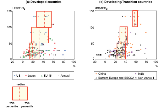
3.4 The role of technologies in long-term mitigation and stabilization: research, development, deployment, diffusion and transfer
Technology is among the central driving forces of GHG emissions. It is one of the main determinants of economic development, consumption patterns and thus human well-being. At the same time, technology and technological change offer the main possibilities for reducing future emissions and achieving the eventual stabilization of atmospheric concentrations of GHGs (see Chapter 2 , Section 2.7.1.2 , which assesses the role of technology in climate change mitigation, including long-term emissions and stabilization scenarios).
The ways in which technology reduces future GHG emissions in long-term emission scenarios include:
- Improving technology efficiencies and thereby reducing emissions per unit service (output). These measures are enhanced when complemented by energy conservation and rational use of energy.
- Replacing carbon-intensive sources of energy by less intensive ones, such as switching from coal to natural gas. These measures can also be complemented by efficiency improvements (e.g. combined cycle natural gas power plants are more efficient than modern coal power plants) thereby further reducing emissions.
- Introducing carbon capture and storage to abate uncontrolled emissions. This option could be applied at some time in the future, in conjunction with essentially all electricity generation technologies, many other energy conversion technologies and energy-intensive processes using fossil energy sources as well as biomass (in which case it corresponds to net carbon removal from the atmosphere).
- Introducing carbon-free renewable energy sources ranging from a larger role for hydro and wind power, photovoltaics and solar thermal power plants, modern biomass (that can be carbon-neutral, resulting in zero net carbon emissions) and other advanced renewable technologies.
- Enhancing the role of nuclear power as another carbon-free source of energy. This would require a further increase in the nuclear share of global energy, depending on the development of ‘inherently’ safe reactors and fuel cycles, resolution of the technical issues associated with long-term storage of fissile materials and improvement of national and international non-proliferation agreements.
- New technology configurations and systems, e.g. hydrogen as a carbon-free carrier to complement electricity, fuel cells and new storage technologies.
- Reducing GHG and CO2 emissions from agriculture and land use in general critically depends on the diffusion of new technologies and practices that could include less fertilizer-intensive production and improvement of tillage and livestock management.
Virtually all scenarios assume that technological and structural changes occur during this century, leading to relative reductions in emissions compared to the hypothetical case of attempting to ‘keep’ emissions intensities of GDP and structure the same as today (see Chapter 2 , Section 2.7.1.1 , which discusses the role of technology in baseline scenarios). Figure 3.32 shows such a hypothetical range of cumulative emissions under the assumption of ‘freezing’ technology and structural change in all scenarios at current levels, but letting populations change and economies develop as assumed in the original scenarios ( Nakicenovic et al., 2006 [SRC] ). To show this, the energy intensity of GDP and the carbon intensity of energy are kept constant. The bars in the figure indicate the central tendencies of the scenarios in the literature by giving the cumulative emissions ranges between the 25th and the 75th percentile of the scenarios in the scenario database. [21] The hypothetical cumulative emissions (without technology and structural change) range from about 9000 (25th percentile) to 1200 0 (75th percentile), with a median of about 1040 0 GtCO2 by 2100 .
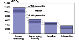
Figure 3.32: Median, 25th and 75th percentile of global cumulative carbon emissions by 2100 in the scenarios developed since 2001 .
The next bar in Figure 3.32 shows cumulative emissions by keeping carbon intensity of energy constant while allowing energy intensity of GDP to evolve as originally specified in the underlying scenarios. This in itself reduces the cumulative emissions substantively, by more than 40% to almost 50% (75th and 25th percentiles, respectively). Thus, structural economic changes and more efficient use of energy lead to significant reductions of energy requirements across the scenarios as incorporated in the baselines, indicating that the baseline already includes vigorous carbon saving. In other words, this means that many new technologies and changes that lead to lower relative emissions are assumed in the baseline. Any mitigation measures and policies need to go beyond these baseline assumptions.
The next bar in Figure 3.32 also allows carbon intensities of energy to change as originally assumed in the underlying scenarios. Again, the baseline assumptions lead to further and substantial reductions of cumulative emissions, by some 13% to more than 20% (25th and 75th percentile, respectively), or less than half the emissions, as compared to the case of no improvement in energy or carbon intensities. This results in the original cumulative emissions as specified by reference scenarios in the literature, from 4050 (25th percentile) to 5400 (75th percentile), with a median of 4730 GtCO2 by 2100 . It should be noted that this range is for the 25th to the 75th percentile only. In contrast, the full range of cumulative emissions across 56 scenarios in the database is from 2075 to 7240 GtCO2. [22]
The next and final step is to compare the cumulative emissions across baseline scenarios with those in the mitigation and stabilization variants of the same scenarios. Figure 3.32 shows (in the last bar) yet another significant reduction of future cumulative emissions from 2370 to 3610 (corresponding to the 25th to the 75th percentile of the full scenario range), with a median of 3010 GtCO2 by 2100 . This corresponds to about 70% emissions reduction across mitigation scenarios, compared to the hypothetical case of no changes in energy and carbon intensities and still a large, or about a 30%, reduction compared to the respective baseline scenarios. [23]
This illustrates the importance of technology and structural changes, both in reference and mitigation scenarios. However, this is an aggregated illustration across all scenarios and different mitigation levels for cumulative emissions. Thus, it is useful to also give a more specific illustrative example. Figure 3.33 gives such an illustration by showing the importance of technological change assumptions in both reference and mitigation scenarios for a 550 ppmv concentration target based on four SRES scenarios. Such analyses are increasingly becoming available. For instance, Placet et al. 2004 [NPR] ) provide a detailed study of possible technology development pathways under climate stabilization for the US government Climate Change Technology Program. To illustrate the importance of technological change, actual projected scenario values in the original SRES no-climate policy scenarios are compared with a hypothetical case with frozen 1990 structures and technologies for both energy supply and end-use. The difference (denoted by a grey shaded area in Figure 3.33 ) illustrates the impact of technological change, which leads to improved efficiency and ‘decarbonization’ in energy systems already incorporated into the baseline emission scenario.
The impacts of technological options leading to emission reductions are illustrated by the colour-shaded areas in Figure 3.33 , regrouped into three categories: demand reductions (e.g. through deployment of more efficient end-use technologies, such as lighting or vehicles), fuel switching (substituting high-GHG-emitting technologies for low- or zero-emitting technologies such as renewables or nuclear), and finally, CO2 capture and storage technologies. The mix in the mitigative technology portfolio required to reduce emissions from the reference scenario level to that consistent with the illustrative 550 ppmv stabilization target varies as a function of the baseline scenario underlying the model calculations (shown in Figure 3.33 ), as well as with the degree of stringency of the stabilization target adopted (not shown in Figure 3.33 ). An interesting finding from a large number of modelling studies is that scenarios with higher degrees of technology diversification (e.g. scenario A1B in Figure 3.33 ) also lead to a higher degree of flexibility with respect of meeting alternative climate (e.g. stabilization) targets and generally also to lower overall costs compared with less diversified technology scenarios. This illustrative example also confirms the conclusion reached in Section 3.3 that was based on a broader range of scenario literature.
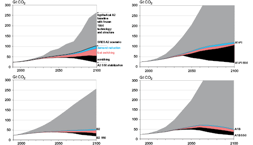
Figure 3.33: Impact of technology on global carbon emissions in reference and climate mitigation scenarios.
This brief assessment of the role of technology across scenarios indicates that there is a significant technological change and diffusion of new and advanced technologies already assumed in the baselines and additional technological change ‘induced’ through various policies and measures in the mitigation scenarios. The newer literature on induced technological change assessed in the previous sections, along with other scenarios (e.g. Grübler et al., 2002 [ARC] ; and Köhler et al., 2006 [NPR, ARC] , see also Chapter 11 ), also affirms this conclusion.
3.4.1 Carbon-free energy and decarbonization
3.4.1.1 Decarbonization trends
Decarbonization denotes the declining average carbon intensity of primary energy over time. Although decarbonization of the world’s energy system is comparatively slow (0.3% per year), the trend has persisted throughout the past two centuries ( Nakicenovic, 1996 [SRC] ). The overall tendency towards lower carbon intensities is due to the continuous replacement of fuels with high carbon content by those with low carbon content; however, intensities are currently increasing in some developing regions. In short- to medium-term scenarios such a declining tendency for carbon intensity may not be as discernable as across the longer-term literature, e.g. in the World Energy Outlook 2004 ( IEA, 2004 [NPR] ), the reference scenario to 2030 shows the replacement of gas for other fossil fuels as well as cleaner fuels due to limited growth of nuclear and bioenergy.
Another effect contributing towards reduced carbon intensity of the economy is the declining energy requirements per unit of GDP, or energy intensity of GDP. Globally, energy intensity has been declining more rapidly than carbon intensity of energy (0.9% per year) during the past two centuries ( Nakicenovic, 1996 [SRC] ). Consequently, carbon intensity of GDP declined globally at about 1.2% per year.
The carbon intensity of energy and energy intensities of GDP were shown in Section 3.2 of this chapter, Figure 3.6 , for the full scenario sample in the scenario database compared to the newer (developed after 2001 ) non-intervention scenarios. As in Sections 3.2 and 3.3 , the range of the scenarios in the literature until 2001 is compared with recent projections from scenarios developed after 2001 ( Nakicenovic et al., 2005 [NPR, SRC] ).
The majority of the scenarios in the literature portray a similar and persistent decarbonization trend as observed in the past. In particular, the medians of the scenario sets indicate energy decarbonization rates of about 0.9% (pre- 2001 literature median) and 0.6% (post- 2001 median) per year, which is a significantly more rapid decrease compared to the historical rates of about 0.3% per year. Decarbonization of GDP is also more rapid (about 2.5% per year for both pre- and post- 2001 literature medians) compared with the historical rates of about 1.2% per year. As expected, the intervention and stabilization scenarios have significantly higher decarbonization rates and the post- 2001 scenarios include a few with significantly more rapid decarbonization of energy, even extending into the negative range. This means that towards the end of the century these more extreme decarbonization scenarios foresee net carbon removal from the atmosphere, e.g. through carbon capture and storage in conjunction with large amounts of biomass energy. Such developments represent a radical paradigm shift compared to the current and more short-term energy systems, implying significant and radical technological changes.
In contrast, the scenarios that are most intensive in the use of fossil fuels lead to practically no reduction in carbon intensity of energy, while all scenarios portray decarbonization of GDP. For example, the upper boundary of the recent scenarios developed after 2001 depict slightly increasing (about 0.3% per year) carbon intensities of energy (A2 reference scenario, ( Mori 2003 ) ), see Figure 3.8 , comparing carbon emissions across scenarios in the literature presented in Section 3.2 ). Most notably, a few scenarios developed before 2001 follow an opposite path compared to other scenarios: decarbonization of primary energy with decreasing energy efficiency until 2040, followed by rapidly increasing ratios of CO2 per unit of primary energy after 2040 – in other words, recarbonization. In the long term, these scenarios lie well above the range spanned by the new scenarios, indicating a shift towards more rapid CO2 intensity improvements in the recent literature ( Nakicenovic et al., 2006 [SRC] ). In contrast, there are just a very few scenarios in the post- 2100 literature that envisage increases in carbon intensity of energy.
The highest rates of decarbonization of energy (up to 2.5% per year for the recent scenarios) are from scenarios that include a complete transition in the energy system away from carbon-intensive fossil fuels. Clearly, the majority of these scenarios are intervention scenarios, although some non-intervention scenarios show drastic reductions in CO2 intensities due to reasons other than climate policies (e.g. the combination of sustainable development policies and technology push measures to promote renewable hydrogen systems). The relatively fast decarbonization rate of intervention scenarios is also illustrated by the median of the post- 2001 intervention scenarios, which depict an average rate of improvement of 1.1% per year over the course of the century, compared to just 0.3% for the non-intervention scenarios. Note, nevertheless, that the modest increase in carbon intensity of energy improvements in the intervention scenarios above the 75th percentile of the distribution of the recent scenarios. The vast majority of these scenarios represent sensitivity analysis; have climate policies for mitigation of non-CO2 greenhouse gas emissions (methane emissions policies: Reilly et al., 2006 [NPR] ); or have comparatively modest CO2 reductions measures, such as the implementation of a relatively minor carbon tax of 10 US$/tC (about 2.7 US$/tCO2) over the course of the century (e.g. ( Kurosawa, 2004 ) ). Although these scenarios are categorized according to our definition as intervention scenarios, they do not necessarily lead to the stabilization of atmospheric CO2 concentrations.
3.4.1.2 Key factors for carbon-free energy and decarbonization development
All of the technological options assumed to contribute towards further decarbonization and reduction of future GHG emissions require further research and development (R&D) to improve their technical performance, reduce costs and achieve social acceptability. In addition, deployment of carbon-saving technologies needs to be applied at ever-larger scales in order to benefit from potentials of technological learning that can result in further improved costs and economic characteristics of new technologies. Most importantly, appropriate institutional and policy inducements are required to enhance widespread diffusion and transfer of these technologies.
Full replacement of dominant technologies in the energy systems is generally a long process. In the past, the major energy technology transitions have lasted more than half a century, such as the transition from coal as the dominant energy source in the world some 80 years ago, to the dominance of crude oil during the 1970 s. Achieving such a transition in the future towards lower GHG intensities is one of the major technological challenges addressed in mitigation and stabilization scenarios.
Figures 3.34 and 3.35 show the ranges of energy technology deployment across scenarios by 2030 and 2100 for baseline (non-intervention) and intervention (including stabilization) scenarios, respectively. The deployment of energy technologies in general, and of new technologies in particular, is significant indeed, even through the 2030 period, but especially by 2100 . The deployment ranges should be compared with the current total global primary energy requirements of some 440 EJ in 2000 . Coal, oil and gas reach median deployment levels ranging from some 150 to 250 EJ by 2030 . The variation is significantly higher by 2100, but even medians reach levels of close to 600 EJ for coal in reference scenarios, thereby exceeding by 50% the current deployment of all primary energy technologies in the world. Deployment of nuclear and biomass is comparatively lower, in the range of about 50–100 EJ by 2030 and up to ten times as much by 2100 . This all indicates that radical technological changes occur across the range of scenarios.
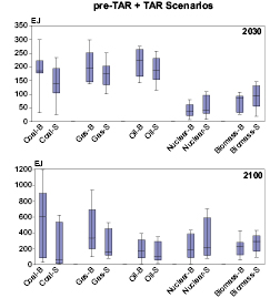
Figure 3.34: Deployment of primary energy technologies across pre- 2001 scenarios by 2030 and 2100 : Left-side ‘error’ bars show baseline (non-intervention) scenarios and right-side ones show intervention and stabilization scenarios. The full ranges of the distributions (full vertical line with two extreme tic marks), the 25th and 75th percentiles (blue area) and the median (middle tic mark) are also shown.
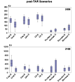
Figure 3.35: Deployment of primary energy technologies across post- 2001 scenarios by 2030 and 2100 : Left-side ‘error’ bars show baseline (non-intervention) scenarios and right-side ones show intervention and stabilization scenarios. The full ranges of the distributions (full vertical line with two extreme tic marks), the 25th and 75th percentiles (blue area) and the median (middle tic mark) are also shown.
The deployment ranges are large for each of the technologies but do not differ much when comparing the pre- 2001 with post- 2001 scenarios over both time periods, up to 2030 and 2100 . Thus, while technology deployments are large in the mean and variance, the patterns have changed little in the new (compared with the older) scenarios. What is significant in both sets of literature is the radically different structure and portfolio of technologies between baseline and stabilization scenarios. Mitigation generally means significantly less coal, somewhat less natural gas and consistently more nuclear and biomass. What cannot be seen from this comparison, due to the lack of data and information about the scenarios, is the extent to which carbon capture and storage is deployed in mitigation scenarios. However, it is very likely that most of the coal and much of the natural gas deployment across stabilization scenarios occurs in conjunction with carbon capture and storage. The overall conclusion is that mitigation and stabilization in emissions scenarios have a significant inducement on diffusion rates of carbon-saving and zero-carbon energy technologies.
3.4.2 RD&D and investment patterns
As mentioned in Chapter 2 , the private sector is leading global research and development of technologies that are close to market deployment, while public funding is essential for the longer term and basic research. R&D efforts in the energy area are especially important for GHG emissions reduction.
Accelerating the availability of advanced and new technologies will be central to greatly reducing CO2 emissions from energy and other sources. Innovation in energy technology will be integral to meeting the objective of emission reduction. Investment and incentives will be needed for all components of the innovation system – research and development (R&D), demonstration, market introduction and its feedback to development, flows of information and knowledge, and the scientific research that could lead to new technological advances.
Thus, sufficient investment will be required to ensure that the best technologies are brought to market in a timely manner. These investments, and the resulting deployment of new technologies, provide an economic value. Model calculations enable economists to quantify the value of improved technologies as illustrated for two technologies in Figure 3.36 .
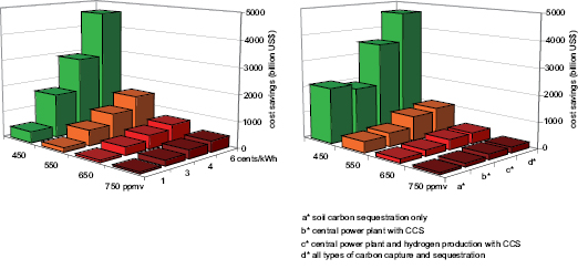
Generally, economic benefits from improved technology increase non-linearly with:
1. The distance to current economic characteristics (or the ones assumed to be characteristic of the scenario baseline).
2. The stringency of environmental targets.
3. The comprehensiveness and diversity of a particular technology portfolio considered in the analysis.
Thus, the larger the improvement of future technology characteristics compared to current ones, the lower the stabilization target, and the more comprehensive the suite of available technologies, the greater will be the economic value of improvements in technology.
These results lend further credence to technology R&D and deployment incentives policies (for example prices [24] ) as ‘hedging’ strategies addressing climate change. However, given the current insufficient understanding of the complexity of driving forces underlying technological innovation and cost improvements, cost-benefit or economic ‘return on investment’, calculations have (to date) not been attempted in the literature, due at least in part to a paucity of empirical technology-specific data on R&D and niche-market deployment expenditures and the considerable uncertainties involved in linking ‘inputs’ (R&D and market stimulation costs) to ‘outputs’ (technology improvements and cost reductions).
3.4.3 Dynamics and drivers of technological change, barriers (timing of technology deployment, learning)
3.4.3.1 Summary from the TAR
The IPCC-TAR concluded that reduction of greenhouse gas emissions is highly dependent on both technological innovation and implementation of technologies (a conclusion broadly confirmed in Chapter 2 , Section 2.7.1 ). However, the rate of introduction of new technologies, and the drivers for adoption are different across different parts of the world, particularly in industrial market economies, economies in transition and developing countries. To some extent this is reflected in global emissions scenarios as they often involve technological change at a level that includes a dozen or so world regions. This usually involves making more region-specific assumptions about future performance, costs and investment needs for new and low-carbon technologies.
There are multiple policy approaches to encourage technological innovation and change. Through regulation of energy markets, environmental regulations, energy efficiency standards, financial and other market-based incentives, such as energy and emission taxes, governments can induce technology changes and influence the level of innovations. In emissions scenarios, this is reflected in assumptions about policy instruments such as taxes, emissions permits, technology standards, costs, and lower and upper boundaries of technology diffusion.
3.4.3.2 Dynamics of technology
R&D, technological learning, and spillovers are the three broad categories of drivers behind technological change. These are discussed in Chapter 2 , Section 2.7 , and Chapter 11 , Section 11.5 . The main conclusion is that, on the whole, all three of the sources of induced technological change (ITC) play important roles in technological advance. Here, we focus on the dynamics of technology and ITC in emissions and stabilization scenarios.
Emissions scenarios generally treat technological change as an exogenous assumption about costs, market penetration and other technology characteristics, with some notable exceptions such as in Gritsevskyi and Nakicenovic 2000 [MoS, SRC] Hourcade and Shukla 2001 [NPR, ARC] ), in their review of scenarios from top-down models, indicate that technology assumptions are a critical factor that affects the timing and cost of emission abatement in the models. They identify widely differing costs of stabilization at 550 ppmv by 2050, of between 0.2 and 1.75% of GDP, mainly influenced by the size of the emissions in the baseline.
The International Modelling Comparison Project (IMCP) ( Edenhofer et al., 2006 [NPR, ARC] ) compared the treatment relating to technological change in many models covering a wide range of approaches. The economies for technological change were simulated in three groups: effects through R&D expenditures, learning-by-doing (LBD) or specialization and scale. IMCP finds that ITC reduces costs of stabilization, but in a wide range, depending on the flexibility of the investment decisions and the range of mitigation options in the models. It should be noted, however, that induced technological change is not a ‘free lunch’, as it requires higher upfront investment and deployment of new technologies in order to achieve cost-reductions thereafter. This can lead to lower overall mitigation costs.
All models indicate that real carbon prices for stabilization targets rise with time in the early years, with some models showing a decline in the optimal price after 2050 due to the accumulated effects of LBD and positive spillovers on economic growth. Another robust result is that ITC can reduce costs when models include low carbon energy sources (such as renewables, nuclear, and carbon capture and sequestration), as well as energy efficiency and energy savings. Finally, policy uncertainty is seen as an issue. Long-term and credible abatement targets and policies will reduce some of the uncertainties around the investment decisions and are crucial to the transformation of the energy system.
ITC broadens the scope of technology-related policies and usually increases the benefits of early action, which accelerates deployment and cost-reductions of low-carbon technologies ( Barker et al., 2006 [NPR, SRC] ; Sijm, 2004 [NPR, MoS] ; Gritsevskyi and Nakicenovic, 2000 [MoS, SRC] ). This is due to the cumulative nature of ITC as treated in the new modelling approaches. Early deployment of costly technologies leads to learning benefits and lower costs as diffusion progresses. In contrast, scenarios with exogenous technology assumptions imply waiting for better technologies to arrive in the future, though this too may result in reduced costs of emission reduction (European Commission, 2003 ).
Other recent work also confirms these findings. For example, Manne and Richels 2004 [SRC] and Goulder 2004 [NPR] ) also found that ITC lowers mitigation costs and that more extensive reductions in GHGs are justified than with exogenous technical change. Nakicenovic and Riahi 2003 [NPR, MoS, SRC] ) noted how the assumption about the availability of future technologies was a strong driver of stabilization costs. Edmonds et al. 2004a [ARC] ) studied stabilization at 550 ppmv CO2 in the SRES B2 world using the MiniCAM model and showed a reduction in costs of a factor of 2.5 in 2100 using a baseline incorporating technical change. Edmonds et al. consider advanced technology development to be far more important as a driver of emission reductions than carbon taxes. Weyant 2004 [SRC] ) concluded that stabilization will require the large-scale development of new energy technologies, and that costs would be reduced if many technologies are developed in parallel and there is early adoption of policies to encourage technology development.
The results from the bottom-up and more technology-specific modelling approaches give a different perspective. Following the work of the IIASA in particular, models investigating induced technical change emerged during the mid- and late- 1990 s. These models show that ITC can alter results in many ways. In the previous sections of this chapter the authors have also illustrated that the baseline choice is crucial in determining the nature (and by implication also the cost) of stabilization. However, this influence is itself largely due to the different assumptions made about technological change in the baseline scenarios. Gritsevskyi and Nakicenovic 2000 [MoS, SRC] ) identified some 53 clusters of least-cost technologies, allowing for endogenous technological learning with uncertainty. This suggests that a decarbonized economy may not cost any more than a carbon-intensive one, if technology learning curves are taken into account. Other key findings are that there is a large diversity across alternative energy technology strategies, a finding that was confirmed in IMCP ( Edenhofer et al., 2006 [NPR, ARC] ). These results suggest that it is not possible to choose an ‘optimal’ direction for energy system development. Some modelling reported in the TAR suggests that a reduction (up to 5 GtC a year) by 2020 (some 50% of baseline projections) might be achieved by current technologies, half of the reduction at no direct cost, the other half at direct costs of less than 100 US$/tC-equivalent (27 US$/tCO2-eq).
3.4.3.3 Barriers to technology transfer, diffusion and deployment for long-term mitigation
Chapter 2 , Section 2.7.2 includes a discussion of the barriers to development and commercialization of technologies. Barriers to technology transfer vary according to the specific context from sector to sector and can manifest themselves differently in developed and developing countries, and in economies-in-transition (EITs). These barriers range from a lack of information; insufficient human capabilities; political and economic barriers (such as the lack of capital, high transaction costs, lack of full cost pricing, and trade and policy barriers); institutional and structural barriers; lack of understanding of local needs; business limitations (such as risk aversion in financial institutions); institutional limitations (such as insufficient legal protection); and inadequate environmental codes and standards.
In the long term, the key drivers of technological change in developing countries will depend on three ‘changes’ that are simultaneous and inseparable within the context of development: exogenous behavioural changes or changes in social infrastructure; endogenous policies driven by ‘development goals’; and any induced change from climate policies ( Shukla et al., 2006 [MoS, SRC] ).
3.4.3.4 Dynamics in developing countries and timing of technology deployment
National policies in developing countries necessarily focus on more fundamental priorities of development, such as poverty alleviation and providing basic living conditions for their populations, and it is unlikely that short-term national policies would be driven by environmental concerns. National policies driven by energy security concerns can, however, have strong alignment with climate goals. The success of policies that address short-term development concerns will determine the pace at which the quality of life in the developing and the developed world converges over the long term.
3.5 Interaction between mitigation and adaptation, in the light of climate change impacts and decision-making under long-term uncertainty
3.5.1 The interaction between mitigation and adaptation, an iterative climate policy process
Responses to climate change include a portfolio of measures:
a. Mitigation – actions that reduce net carbon emissions and limit long-term climate change.
b. Adaptation – actions that help human and natural systems to adjust to climate change.
c. Research on new technologies, on institutional designs and on climate and impacts science, which should reduce uncertainties and facilitate future decisions ( Richels et al., 2004 [NPR, SRC] ; Caldeira et al., 2003 [JoC] ; Yohe et al., 2004 [JoC, MoS] ).
A key question for policy is what combination of short-term and long-term actions will minimize the total costs of climate change, in whatever form these costs are expressed, across mitigation, adaptation and the residual climate impacts that society is either prepared or forced to tolerate. Although there are different views on the form and dynamics of such trade-offs in climate policies, there is a consensus that they should be aligned with (sustainable) development policies, since the latter determine the capacity to mitigate and to adapt in the future (TAR, Hourcade and Shukla, 2001 [NPR, ARC] ). In all cases, policy decisions will have to be made with incomplete understanding of the magnitude and timing of climate change, of its likely consequences, and of the cost and effectiveness of response measures.
3.5.1.1 An iterative risk-management framework to articulate options
Previous IPCC reports conclude that climate change decision-making is not a once-and-for-all event, but an iterative risk-management process that is likely to take place over decades, where there will be opportunities for learning and mid-course corrections in the light of new information ( Lempert et al., 1994 [JoC] ; Keller et al., 2006 [JoC] ).
This iterative process can be described using a decision tree ( Figure 3.37 ), where the square nodes represent decisions, the circles represent the reduction of uncertainty and the arrows indicate the range of decisions and outcomes. Some nodes summarize today’s options – how much should be invested in mitigation, in adaptation, in expanding mitigative and adaptive capacity, or in research to reduce uncertainty? Other nodes represent opportunities to learn and make mid-course corrections. This picture is a caricature of real decision processes, which are continuous, overlapping and iterative. However, it is useful to conceptually put the many determinants of any short-term strategy in a context of progressive resolution of uncertainty.
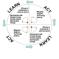
3.5.1.2 Qualitative insights into interactions between mitigaton, adaptation and development
Until recently, a main focus in the policy and integrated assessment literature has been on comparing mitigation costs and avoided damages. Since the TAR, attention has shifted towards the interaction between mitigation and adaptation in reducing damages in a risk-management framework. This has accompanied a growing realization that some climate change in the coming decades is inevitable.
Limited treatment of adaptation in climate policy assessments is still a problem and a number of reasons explain this. First, the focus of the international climate change negotiations has largely been on mitigation (perhaps because attention to adaptation could be viewed as ‘giving up’ on mitigation) even though the importance of adaptation is underlined in Article 4 of the UNFCCC and Article 10 of the Kyoto Protocol. Second, adaptation is largely undertaken at the local scale, by individual households, farmers, companies or local governments; it is thus difficult to target through coordinated international incentives, and is more complicated to handle quantitatively by models in global scenarios. Third, it is difficult to generalize the ways that individuals or communities are likely to adapt to specific impacts. However, the literature is evolving quickly and recent work is available in a number of regions; for example, in Finland ( Carter et al., 2005 [NPR, MoS] ), the UK ( West and Gawith, 2005 [NPR] ), Canada ( Cohen et al., 2004 [NPR] ) and the USA (e.g. California, Hayhoe et al., 2004 [PoC, JoC, ARC] ).
Despite the scarcity of global systematic assessments ( (Tol, 2005a ) ), some interesting insights into the interaction between adaptation and mitigation emerge from recent regional-scale studies. Some adaptation measures are ‘no-regret’ measures and should be undertaken anyway ( Agrawala, 2005 [NPR] ), such as preservation of mangroves in coastal zones, which provide a buffer for increased coastal flood risk due to climate change and help to maintain healthy marine ecosystems ( Nicholls et al., 2006 [NPR] ). A few may be synergistic with mitigation ( Bosello, 2005 [NPR] ) such as investing in more efficient buildings that will limit human vulnerability to increasingly frequent heatwaves and also reduce energy use, hence emissions. But many adaptation options involve net costs with a risk of committing to irreversible and misplaced investment given the considerable uncertainty about climate change at a local scale. Given this uncertainty, and the fact that learning about adaptation to climate change imposes some costs and takes time ( Kelly et al., 2005 [ARC] ), mis-allocation of investments may occur, or the rate of long-term investment in adaptation strategies may slow ( Kokic et al., 2005 [MoS, SRC] ; Kelly et al., 2005 [ARC] ).
Finally, the interactions between adaptation and mitigation are intertwined with development pathways. A key issue is to understand at what point (over)investment in mitigation or adaptation might limit funds available for development, and thus reduce future adaptive capacity ( Sachs, 2004 [JoC] ;( Tol, 2005a; ) Tol and Yohe, 2006 [NPR] ). Another issue concerns the point at which climate change damages, and the associated investment in adaptation, could crowd out more productive investments later and harm development ( (Kemfert, 2002; ) Bosello and Zhang, 2005 [NPR] ; Kemfert and Schumacher, 2005 [NPR] ). The answer to these questions depends upon modelling assumptions that drive repercussions in other sectors of the economy and other regions and the potential impacts on economic growth. These are ‘higher-order’ social costs of climate change from a series of climate-change-induced shocks; they include the relative influence of: a) the cross-sectoral interactions across all major sectors and regions; b) a crowding out effect that slows down capital accumulation and technical progress, especially if technical change is endogenous. These indirect impacts reduce development and adaptive capacity and may be in the same order of magnitude, or greater than, the direct impact of climate change ( Fankhauser and Tol, 2005 [JoC] ; Roson and Tol, 2006 [MoS] ; Kemfert, 2006 [MoS] ).
Both the magnitude and the sign of the indirect macro-economic impacts of climate change are conditional upon the growth dynamics of the countries concerned. When confronted by the same mitigation policies and the same climate change impacts, economies experiencing strong disequilibrium (including ‘poverty traps’) and large market and institutional imperfections will not react in the same way as countries that are on a steady and high economic growth pathway. The latter are near what economists call their ‘production frontier’ (the maximum of production attainable at a given point in time); the former are more vulnerable to any climatic shock or badly calibrated mitigation policies, but symmetrically offer more opportunities for synergies between mitigation, adaptation and development policies ( Shukla et al., 2006 [MoS, SRC] ). On the adaptation side for example, ( Tol and Dowlatabadi 2001 ) ) demonstrate that there is significant potential to reduce vulnerability to the spread of malaria in Africa. In some circumstances, mitigation measures can be aligned with development policies and alleviate important sources of vulnerability in these countries, such as dependency on oil imports or local pollution. But this involves transition costs over the coming 10–20 years (higher domestic energy prices, higher investments in the energy sector), which in turn suggests opportunities for international cooperative mechanisms to minimize these costs.
Bosello 2005 [NPR] ) shows complementarity between adaptation, mitigation and investment in R&D, whilst others consider these as substitutes ( (Tol, 2005a ) Schneider and Lane 2006 [NPR, PoC] ) consider that mitigation and adaptation only trade off for small temperature increments where adaptation might be cheaper, whereas for larger temperature increases mitigation is always the cheaper option. ( Goklany 2003 ) ) promotes the view that the contribution by climate change to hunger, malaria, coastal flooding, and water stress (as measured by populations at risk) is small compared to that of non-climate-change-related factors, and that through the 2080 s, efforts to reduce vulnerability would be more cost-effective in reducing these problems than mitigation. This analysis neglects critical thresholds at the regional level (such as the temperature ceiling on feasibility of regional crop growth) and at the global level (such as the onset of ice sheet melting or release of methane from permafrost), and, like many others studies, it neglects the impacts of extreme weather events. It also promotes a very optimistic view of adaptive capacity, which is increasingly challenged in the literature ( (Tompkins and Adger, 2005 ) ). An adaptation-only policy scenario in the coming decades leads to an even greater challenge for adaptation in decades to follow, owing to the inertia of the climate system. In the absence of mitigation, temperature rises will be much greater than would otherwise occur with pusuant impacts on economic development ( IPCC, 2007b [NPR, 2007] , Chapter 19.3.7; Stern 2006 [NPR] ). Hence adaptation alone is insufficient to avoid the serious risks due to climate change (see Table 3.11 ; also IPCC, 2007b [NPR, 2007] , Chapter 19, Table 19.1).
To summarize, adaptation and mitigation are thus increasingly viewed as complementary (on the global scale), whilst locally there are examples of both synergies and conflicts between the two ( IPCC, 2007b [NPR, 2007] , Chapter 18). Less action on mitigation raises the risk of greater climate-change-induced damages to economic development and natural systems and implies a greater need for adaptation. Some authors maintain that adaptation and mitigation are substitutes, because of competition for funds, whilst others claim that such tradeoffs occur only at the margin when considering incremental temperature change and incremental policy action, because for large temperature changes mitigation is always cheaper than adaptation.
Table 3.9: Global mean temperature increase at equilibrium, greenhouse gas concentration and radiative forcing. Equilibrium temperatures here are calculated using estimates of climate sensitivity and do not take into account the full range of bio-geophysical feedbacks that may occur.
| Equilibrium temperature increase in ºC above pre-industrial temperature | CO2-eq concentration and radiative forcing corresponding to best estimate of climate sensitivity for warming level in column 11,2 | CO2-eq concentration that would be expected to limit warming below level in column 1 with an estimated likelihood of about 80% 3 | |
|---|---|---|---|
| CO2-equivalent (ppm) | Radiative forcing (W/m2) | ||
| 0.6 | 319 | 0.7 | 305 |
| 1.6 | 402 | 2.0 | 356 |
| 2.0 | 441 | 2.5 | 378 |
| 2.6 | 507 | 3.2 | 415 |
| 3.0 | 556 | 3.7 | 441 |
| 3.6 | 639 | 4.5 | 484 |
| 4.0 | 701 | 4.9 | 515 |
| 4.6 | 805 | 5.7 | 565 |
| 5.0 | 883 | 6.2 | 601 |
| 5.6 | 1014 | 6.9 | 659 |
| 6.0 | 1112 | 7.4 | 701 |
| 6.6 | 1277 | 8.2 | 768 |
3.5.2 Linking emission scenarios to changes in global mean temperature, impacts and key vulnerabilities
In a risk-management framework, a first step to understanding the environmental consequences of mitigation strategies is to look at links between various stabilization levels for concentrations of greenhouse gases in the atmosphere, and the global mean temperature change relative to a particular baseline. A second step is to link levels of temperature change and key vulnerabilities. Climate models indicate significant uncertainty at both levels. Figure 3.38 shows CO2-eq concentrations that would limit warming at equilibrium below the temperatures indicated above pre-industrial levels, for ‘best estimate’ climate sensitivity, and for the likely range of climate sensitivity (see Meehl et al., 2007 [NPR, MoS, 2007] , Section 10.7, and Table 10.8; and the notes to Figure 3.38). It also shows the corresponding radiative forcing levels and their relationship to equilibrium temperature and CO2-eq concentrations. The table and the figure illustrate how lower temperature constraints require lower stabilization levels, and also that, if the potential for climate sensitivities is higher than the ‘best estimate’ and is taken into account, the constraint becomes more stringent. These more stringent constraints lower the risks of exceeding the threshold.
Figure 3.38 and Table 3.10 provide an overview of how emission scenarios ( Section 3.3 ) relate to different stabilization targets and to the likelihood of staying below certain equilibrium warming levels. For example, respecting constraints of 2°C above pre-industrial levels, at equilibrium, is already outside the range of scenarios considered in this chapter, if the higher values of likely climate sensitivity are taken into account (red curve in Figure 3.38 ), whilst a constraint of respecting 3°C above pre-industrial levels implies the most stringent of the category I scenarios, with emissions peaking in no more than the next 10 years, again if the higher likely values of climate sensitivity are taken into account. Using the ‘best estimate’ of climate sensitivity (i.e. the estimated mode) as a guide for establishing targets, implies the need for less stringent emission constraints. This ‘best estimate’ assumption shows that the most stringent (category I) scenarios could limit global mean temperature increases to 2°C–2.4°C above pre-industrial levels, at equilibrium, requiring emissions to peak within 10 years. Similarly, limiting temperature increases to 2°C above pre-industrial levels can only be reached at the lowest end of the concentration interval found in the scenarios of category I (i.e. about 450 ppmv CO2-eq using ‘best estimate’ assumptions). By comparison, using the same ‘best estimate’ assumptions, category II scenarios could limit the increase to 2.8°C–3.2°C above pre-industrial levels at equilibrium, requiring emissions to peak within the next 25 years, whilst category IV scenarios could limit the increase to 3.2°C–4°C above pre-industrial at equilibrium requiring emissions to peak within the next 55 years. Note that Table 3.10 category IV scenarios could result in temperature increases as high as 6.1°C above pre-industrial levels, when the likely range for the value of climate sensitivity is taken into account. Hence, setting policy on the basis of a ‘best estimate’ climate sensitivity accepts a significant risk of exceeding the temperature thresholds, since the climate sensitivity could be higher than the best estimate.
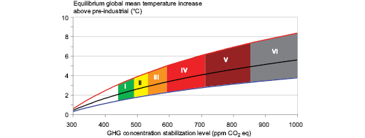
Figure 3.38: Relationship between global mean equilibrium temperature change and stabilization concentration of greenhouse gases using: (i) ‘best estimate’ climate sensitivity of 3°C (black), (ii) upper boundary of likely range of climate sensitivity of 4.5°C (red), (iii) lower boundary of likely range of climate sensitivity of 2°C (blue) (see also Table 3.9).
Table 3.10: Properties of emissions pathways for alternative ranges of CO2 and CO2-eq stabilization targets. Post-TAR stabilization scenarios in the scenario database (see also Sections 3.2 and 3.3 ); data source: after Nakicenovic et al., 2006 [SRC] and Hanaoka et al., 2006 [NPR, SRC] )
| Class | Anthropogenic addition to radiative forcing at stabilization (W/m2) | Multi-gas concentration level (ppmv CO2-eq) | Stabilization level for CO2 only, consistent with multi-gas level (ppmv CO2) | Number of scenario studies | Global mean temperature C increase above pre-industrial at equilibrium, using best estimate of climate sensitivityc) | Likely range of global mean temperature C increase above pre-industrial at equilibriuma) | Peaking year for CO2 emissionsb) | Change in global emissions in 2050 (% of 2000 emissions)b) |
|---|---|---|---|---|---|---|---|---|
| I | 2.5-3.0 | 445-490 | 350-400 | 6 | 2.0-2.4 | 1.4-3.6 | 2000-2015 | -85 to -50 |
| II | 3.0-3.5 | 490-535 | 400-440 | 18 | 2.4-2.8 | 1.6-4.2 | 2000-2020 | -60 to -30 |
| III | 3.5-4.0 | 535-590 | 440-485 | 21 | 2.8-3.2 | 1.9-4.9 | 2010-2030 | -30 to +5 |
| IV | 4.0-5.0 | 590-710 | 485-570 | 118 | 3.2-4.0 | 2.2-6.1 | 2020-2060 | +10 to +60 |
| V | 5.0-6.0 | 710-855 | 570-660 | 9 | 4.0-4.9 | 2.7-7.3 | 2050-2080 | +25 to +85 |
| VI | 6.0-7.5 | 855-1130 | 660-790 | 5 | 4.9-6.1 | 3.2-8.5 | 2060-2090 | +90 to +140 |
Table 3.11 highlights a number of climate change impacts and key vulnerabilities organized as a function of global mean temperature rise ( IPCC, 2007b [NPR, 2007] , Chapter 19). The table highlights a selection of key vulnerabilities representative of categories covered in Chapter 19 (Table 19.1) in IPCC 2007b [NPR, 2007] ). The italic text in Table 3.11 highlights examples of avoided impacts derived from ensuring that temperatures are constrained to any particular temperature range compared to a higher one. For example, significant benefits result from constraining temperature change to not more than 1.6°C–2.6°C above pre-industrial levels. These benefits would include lowering (with different levels of confidence) the risk of: widespread deglaciation of the Greenland Ice Sheet; avoiding large-scale transformation of ecosystems and degradation of coral reefs; preventing terrestrial vegetation becoming a carbon source; constraining species extinction to between 10–40%; preserving many unique habitats (see IPCC, 2007b [NPR, 2007] , Chapter 4, Table 4.1 and Figure 4.5) including much of the Arctic; reducing increases in flooding, drought, and fire; reducing water quality declines, and preventing global net declines in food production. Other benefits of this constraint, not shown in the Table 3.11 , include reducing the risks of extreme weather events, and of at least partial deglaciation of the West Antarctic Ice Sheet (WAIS), see also IPCC, 2007b [NPR, 2007] , Section 19.3.7. By comparison, for ‘best guess’ climate sensitivity, attaining these benefits becomes unlikely if emission reductions are postponed beyond the next 15 years to a time period between the next 15–55 years. Such postponement also results in increasing risks of a breakdown of the Meridional Overturning Circulation ( IPCC, 2007b [NPR, 2007] , Table 19.1).
Even for a 2.6°C –3.6°C temperature rise above pre-industrial levels there is also medium confidence in net negative impacts in many developed countries ( IPCC, 2007b [NPR, 2007] , Section 19.3.7). For emission-reduction scenarios resulting in likely temperature increases in excess of 3.6°C above pre-industrial levels, successively more severe impacts result. Low temperature constraints are necessary to avoid significant increases in the impacts in less developed regions of the world and in polar regions, since many market sectors in developing countries are already affected below 2.6°C above pre-industrial levels ( IPCC, 2007b [NPR, 2007] , Section 19.3.7), and indigenous populations in high latitude areas already face significant adverse impacts.
It is possible to use stablization metrics (i.e. global mean temperature increase, concentrations in ppmv CO2-eq or radiative forcing in W/m2) in combination with the mitigation scenarios literature to assess the cost of alternative mitigation pathways that respect a given equilibrium temperature, key vulnerability (KV) or impact threshold. Whatever the target, both early and delayed-action mitigation pathways are possible, including ‘overshoot’ pathways that temporarily exceed this level. A delayed mitigation response leads to lower discounted costs of mitigation, but accelerates the rate of change and the risk of transiently overshooting pre-determined targets ( IPCC, 2007b [NPR, 2007] , Section 19.4.2).
A strict comparison between mitigation scenarios and KVs is not feasible as the KVs in Table 3.11 refer to realized transient temperatures in the 21st century rather than equilibrium temperatures, but a less rigorous comparison is still useful. Avoidance of many KVs requires temperature change in 2100 to be below 2°C above 1990 levels (or 2.6°C above pre-industrial levels). Using equilibrium temperature as a guide, impacts or KV could be less than expected, for example if impacts do not occur until the 22nd century, because there is more time for adaptation. Or they might be greater than expected, as temperatures in the 21st century may transiently overshoot the equilibrium, or stocks at risk (such as human populations) might be larger. Some studies explore the link between transient and equilibrium temperature change for alternative emission pathways ( O’Neill and Oppenheimer, 2004 [SRC] ; Schneider and Mastrandrea, 2005 [PoC, JoC, SRC] ; Meinshausen, 2006 [NPR, MoS] ).
It is transient climate change, rather than equilibrium change, that will drive impacts. More research is required to address the question of emission pathways and transient climate changes and their links to impacts. [25] In the meantime, equilibrium temperature change may be interpreted as a gross indicator of change, and given the caveats above, as a rough guide for policymakers’ consideration of KV and mitigation options to avoid KV.
| GMT range relative to 1990 (pre-industrial) | Geophysical systems Example: Greenland ice sheeta (IPCC, 2007b: 6.3; 19.3.5.2; IPCC, 2007a: 4.7.4; 6.4.3.3; 10.7.4.3; 10.7.4.4) | Global biological systems Example: terrestrial ecosystemsb (IPCC, 2007b: 4.4.11; 1.3.4; 1.3.5) | Global social systems Example: waterc (IPCC, 2007b: 3 ES; 3.4.3; 13.4.3) | Global social systems Example: food supplyc (IPCC, 2007b: 5.6.1; 5.6.4) | Regional systems Example: Polar Regionsd (IPCC, 2007b: 15.4.1; 15.4.2; 15.4.6; 15.4.7) | Extreme events Example: fire riske (IPCC, 2007a: 7.3; IPCC, 2007b; 1.3.6) |
|---|---|---|---|---|---|---|
| >4 (>4-6) | Near-total deglaciation** | Large-scale transformation of ecosystems and ecosystem services** At least 35% of species committed to extinction (3°C)** | Severity of floods, droughts, erosion, water quality deterioration will increase with increasing climate change*** | Further declines in global food production o/* | Continued warming likely to lead to further loss of ice cover and permafrost**. Arctic ecosystems further threatened**, although net ecosystem productivity estimated to increase (o) | Frequency and intensity likely to be greater, especially in boreal forests and dry peat lands after melting of permafrost** |
| 3-4 (3.6-4.6) | Commitment to widespread** to near-total deglaciation* 2-7 m sea level rise over centuries to millennia | Global vegetation becomes net source of C above 2-3ºC */** | Sea level rise will extend areas of salinization of ground water, decreasing freshwater availability in coastal areas*** | While some economic opportunities will open up (e.g. shipping), traditional ways of life will be disrupted** | ||
| 2-3 (2.6-3.6) | Lowers risk of near-total deglaciation | Widespread disturbance, sensitive to rate of climate change and land use*** 20 to 50% species committed to extinction* Avoids widespread disturbance to ecosystems and their services***, and constrains species losses | Hundreds of millions people would face reduced water supplies (**) | Global food production peaks and begins to decrease o/* (1-3ºC) Lowers risk of further declines in global food production associated with higher temperatures* | ||
| 1-2 (1.6-2.6) | Localized deglaciation (already observed due to local warming), extent would increase with temperature** | 10-40% of species committed to extinction* Reduces extinctions to below 20-50%*, prevents vegetation becoming carbon source*/** Many ecosystems already affected*** | Increased flooding and drought severity** Lowers risk of floods, droughts, deteriorating water quality*** and reduced water supplied for hundreds of millions of people** | Reduced low latitude production*. Increased high latitude production* (1-3ºC) | Climate change is already having substantial impacts on societal and ecological systems*** | Increased fire frequency and intensity in many areas, particularly where drought increases** |
| 0-1 (0.6-1.6) | Lowers risk of widespread** to near-total deglaciation* | Reduces extinctions to below 10-30%*; reduces disturbance levels*** | Increased global production o/* Lowers risk of decrease in global food production and reduces regional losses (or gains) o/* | Reduced loss of ice cover and permafrost; limits risk to Arctic ecosystems and limits disruption of traditional ways of life** | Lowers risk of more frequent and more intense fires in many areas** | |
3.5.3 Information for integrated assessment of response strategies
Based upon a better understanding of the links between concentration levels, magnitude and rate of warming and key vulnerabilities, the next step in integrated assessment is to make informed decisions by combining information on climate science, impact analysis and economic analysis within a consistent analytical framework. These exercises can be grouped into three main categories depending on the way uncertainty is dealt with, the degree of complexity and multi-disciplinary nature of models and on the degree of ambition in terms of normative insights:
1. Assessment and sensitivity analysis of climate targets.
2. Inverse analyses to determine emission-reduction corridors (trajectories) to avoid certain levels of climate change or of climate impacts.
3. Monetary assessment of climate change damages.
Section 3.6 discusses how this information is used in economic analyses to determine optimal emission pathways.
3.5.3.1 Scenario and sensitivity analysis of climate targets
Probabilistic scenario analysis can be used to assess the risk of overshooting some climate target or to produce probabilistic projections that quantify the likelihood of a particular outcome. Targets for such analysis can be expressed in several different ways: absolute global mean temperature rise by 2100, rate of climate change, other thresholds beyond which dangerous anthropogenic interference (DAI) may occur, or additional numbers of people at risk to various stresses. For example, Arnell et al. 2002 [JoC] ) show that such stresses (conversion of forests to grasslands, coastal flood risk, water stress) are far less at 550 ppmv than at 750 ppmv.
Recent Integrated Assessment Models (IAM) literature reflects a renewed attention to climate sensitivity as a key driver of climate dynamics (Den Elzen and Meinshausen, 2006 [NotFound] ; Hare and Meinshausen, 2006 [JoC, ARC] ; Harvey, 2006 [JoC] ; Keller et al., 2006 [JoC] ; Mastrandrea and Schneider, 2004 [PoC, JoC, SRC] ; Meehl et al., 2005 [JoC] ; Meinshausen et al., 2006 [NPR, MoS] , Meinshausen, 2006 [NPR, MoS] ; O’Neill and Oppeinheimer, 2002, 2004; Schneider and Lane, 2004 [NPR, PoC] ; Wigley, 2005 [JoC] ). The consideration of a full range of possible climate sensitivity increases the probability of exceeding thresholds for specific DAI. It also magnifies the consequence of delaying mitigation efforts. Hare and Meinshausen 2006 [JoC, ARC] ) estimate that each 10-year delay in mitigation implies an additional 0.2°C–0.3°C warming over a 100–400 year time horizon. For a climate sensitivity of 3°C, Harvey 2006 [JoC] ) shows that immediate mitigation is required to constrain temperature rise to roughly 2°C above pre-industrial levels. Only in the unlikely situation where climate sensitivity is 1°C or lower would immediate mitigation not be necessary. [26] Harvey also points out that, even in the case of a 2°C threshold (above pre-industrial levels), acidification of the ocean would still occur and that this might not be considered safe.
Another focus of sensitivity analysis is on mitigation scenarios that overshoot and eventually return to a given stabilization or temperature target ( Kheshgi, 2004 [ARC] ; Wigley, 2005 [JoC] ; Harvey, 2004 [JoC] ; Izrael and Semenov, 2005 [MoS] ; Kheshgi et al., 2005 [ARC] ; Meinshausen et al., 2006 [NPR, MoS] Schneider and Mastrandrea 2005 [PoC, JoC, SRC] ) find that this risk of exceeding a threshold of 2ºC above pre-industrial levels is increased by 70% for an overshoot scenario stabilizing at 500 ppmv CO2-eq (as compared to a scenario stabilizing at 500 ppmv CO2-eq). Such overshoot scenarios are likely to be necessary if there is a decision to achieve stablization of GHG concentrations close to (or at) today’s levels. They are indeed likely to lower the costs of mitigation but, in turn, raise the risk of exceeding such thresholds ( Keller et al., 2006 [JoC] ; Schneider and Lane, 2004 [NPR, PoC] ) and may limit the ability to adapt by increasing the rate of climate change, at least temporarily ( Hare and Meinshausen, 2006 [JoC, ARC] O’Neill and Oppenheimer 2004 [SRC] ) find that the transient temperature up to 2100 is equally, or more, controlled by the pathway to stabilization than by the stabilization target, and that overshooting can lead to a peak temperature increase that is higher than in the long-term (equilibrium) warming.
The last and important contribution of this approach is to test the sensitivity of results to carbon cycle and climate change feedbacks ( Cox et al., 2000 [JoC, MoS] ; Friedlingstein et al., 2001 [MoS] ;( Matthews, 2005 ) ) and other factors that may affect carbon cycle dynamics, such as deforestation ( Gitz and Ciais, 2003 [NPR, MoS] ). For example, carbon cycle feedbacks amplify warming ( Meehl et al., 2007 [NPR, MoS, 2007] ) and are omitted from most other studies that thus underestimate the risks of exceeding (or overshooting) temperature targets for a given effort of mitigation in the energy sector only. This could increase warming by up to 1°C in 2100, according to a simple model ( Meehl et al., 2007 [NPR, MoS, 2007] ). The amplification, together with further potential amplification due to feedbacks of uncertain magnitude, such as the potential release of methane from permafrost, peat bogs and seafloor clathrates ( Meehl et al., 2007 [NPR, MoS, 2007] ) are also not included in the analysis presented in Figure 3.38 and Table 3.10 . This analysis reflects only known feedbacks for which the magnitude can be estimated and are included in General Circulation Models (GCMs). Hence, scenario and sensitivity analysis shows that the risks of exceeding a given temperature threshold for a given temperature target may be higher than that shown in Table 3.10 and Figure 3.38 .
3.5.3.2 Inverse modelling and guardrail analysis
Inverse modelling approaches such as Safe Landing Analysis ( Swart et al., 1998 [NPR, MoS] ) and Tolerable Windows Approach ( Toth, 2003 [JoC, SRC] ), aim to define a guardrail of allowable emissions for sets of unacceptable impacts or intolerable mitigation costs. They explore how the set of viable emissions pathways is constrained by parameters such as the starting date, the rate of emission reductions, or the environmental constraints. They provide insights into the influence of short-term decisions on long-term targets by delineating allowable emissions corridor, but they do not prescribe unique emissions pathways, as per cost-effectiveness or costs-benefit analysis.
For example, Toth et al. 2002 [SRC] ) draw on climate impact response functions (CIRFs) by ( Füssel and van Minnen 2001 ) ) that use detailed biophysical models to estimate regionally specific, non-monetized impacts for different sectors (i.e. agricultural production, forestry, water runoff and biome changes). They show that the business-as-usual scenario of GHG emissions (which resembles the SRES A2 scenario) to 2040 precludes the possibility of limiting the worldwide transformation of ecosystems to 30% or less, even with very high willingness to pay for the mitigation of GHG emissions afterwards. Some applications of guardrail analyses assess the relationship between emission pathways and abrupt change such as thermohaline circulation (THC) collapse ( Rahmstorf and Zickfeld, 2005 [PoC, JoC] ). The latter study concludes that stringent mitigation policy reduces the probability of THC collapse but cannot entirely avoid the risk of shutdown.
Corfee-Morlot and Höhne 2003 [JoC, ARC] ) conclude that only low stabilization targets (e.g. 450 ppmv CO2 or 550 ppmv CO2-eq) significantly reduce the likelihood of climate change impacts. They use an inverse analysis to conclude that more than half of the SRES (baseline) emission scenarios leave this objective virtually out of reach as of 2020 .
More generally, referring to Table 3.10 , if the peaking of global emissions is postponed beyond the next 15 years to a time period somewhere between the next 15–55 years, then constraining global temperature rise to below 2°C above 1990 (2.6°C above pre-industrial levels) becomes unlikely (using ‘best estimate’ assumptions of climate sensitivity), resulting in increased risks of the impacts listed in Table 3.11 and discussed in Section 3.5.2 .
3.5.3.3 Cost-benefit analysis, damage cost estimates and social costs of carbon
The above analysis provides a means of eliminating those emissions scenarios that are outside sets of pre-determined guardrails for climate protection and provides the raw material for cost-effectiveness analysis of optimal pathways for GHG emissions. If one wants to determine these pathways through a cost-benefit analysis it is necessary to assess the trade-off between mitigation, adaptation and damages, and consequently, to measure damages in the same monetary metric as mitigation and adaptation expenditures. Such assessment can be carried out directly in the form of ‘willingness to pay for’ avoiding certain physical consequences.
Some argue that it is necessary to specify more precisely why certain impacts are undesirable and to comprehensively itemize the economic consequences of climate change in monetary terms. The credibility of such efforts has often been questioned, given the uncertainty surrounding climate impacts and the efficacy of societal responses to them, plus the controversial meaning of a monetary metric across different regions and generations ( Jacoby, 2004 [JoC, MoS] ). This explains why few economists have taken the step of monetizing global climate impacts. At the time of the TAR, only three such comprehensive studies had been published ( Mendelsohn et al., 2000 [JoC] ; Nordhaus and Boyer, 2000 [NPR, MoS] ; and Tol, 2002a [MoS] , 2002b ). Their estimates ranged from negligible to 1.5% of the GDP for a global mean temperature rise of +2.5°C and Nordhaus and Boyer carefully warned: ‘Along the economically efficient emission path, the long-run global average temperature after 500 years is projected to increase 6.2°C over the 1900 global climate. While we have only the foggiest idea of what this would imply in terms of ecological, economic, and social outcomes, it would make the most thoughtful people, even economists, nervous to induce such a large environmental change. Given the potential for unintended and potentially disastrous consequences….’
Progress has been made since the TAR in assessing the impacts of climate change. Nonetheless, as noted in Watkiss et al. 2005 [NPR, MoS] ), estimates of the social costs of carbon (SCC) in the recent literature still reflect an incomplete subset of relevant impacts; many significant impacts have not yet been monetized (see also IPCC, 2007b [NPR, 2007] ; for SCC see IPCC 2007b [NPR, 2007] , Section 20.6) and others are calibrated in numeraires that may defy monetization for some time to come. Existing reviews of available SCC estimates show that they span several orders of magnitude – ranges that reflect uncertainties in climate sensitivity, response lags, discount rates, the treatment of equity, the valuation of economic and non-economic impacts, and the treatment of possible catastrophic losses ( IPCC, 2007b [NPR, 2007] , Chapter 20). The majority of available estimates in the literature also capture only impacts driven by lower levels of climate change (e.g. 3°C above 1990 levels). IPCC 2007b [NPR, 2007] ) highlights available estimates of SCC that run from -3 to 95 US$ /tCO2 from one survey, but also note that another survey includes a few estimates as high as 400 US$/tCO2 ( IPCC, 2007b [NPR, 2007] , Chapter 20, ES and Section 20.6.1). However the lower boundary of this range includes studies where climate change is presumed to be low and aggregate benefits accrue. Moreover, none of the aggregate estimates reflect the significant differences in impacts that will be felt across different regions; nor do they capture any of the social costs of other greenhouse gases. A more recent estimate by Stern 2006 [NPR] ) is at the high end of these estimates (at 85 US$/tCO2) because an extremely low discount rate (of 1.4%) is used in calculating damages that include additional costs attributed to abrupt change and increases in global mean temperature for some scenarios in excess of 7°C ( Nordhaus, 2006a [JoC] ; Yohe, 2006 [MoS] ; Tol and Yohe, 2006 [NPR] ). The long-term high-temperature scenarios are due to inclusion of feedback processes. IPCC 2007b [NPR, 2007] ) also highlights the fact that the social costs of carbon and other greenhouse gases could increase over time by 2–4% per year ( IPCC, 2007b [NPR, 2007] ; Chapter 20, ES and Section 20.6.1).
For a given level of climate change, the discrepancies in estimates of the social costs of carbon can be explained by a number of parameters highlighted in Figure 3.39 . These stem from two different types of questions: normative and empirical. Key normative parameters include the inter-temporal aggregation of damages through discount rates and aggregation methods for impacts across diverse populations within the same time period ( Azar and Lindgren, 2003 [JoC] ; Howarth, 2003 [JoC] ; Mastrandrea and Schneider, 2004 [PoC, JoC, SRC] ) and are responsible for much of the variation.
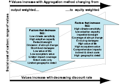
The other parameters relate to the empirical validity of their assessment, given the poor quality of data and the difficulty of predicting how society will react to climate impacts in a given sector, at a given scale in future decades. ( Pearce 2003 ) ) suggests that climate damages and SCC may be over-estimated due to the omission of possible amenity benefits in warmer climates or high-latitude regions ( Maddison 2001 [NPR] ) and possible agricultural benefits. However, overall, it is likely that current SCC estimates are understated due to the omission of significant impacts that have not yet been monetized ( IPCC, 2007b [NPR, 2007] , Chapters 19 and 20; Watkiss et al., 2005 [NPR, MoS] ).
Key empirical parameters that increase the social value of damages include:
- Climate sensitivity and response lag. Equilibrium temperature rise for a doubling of CO2, and the modelled response time of climate to such a change in forcing. Hope (2006) in his PAGE 2002 model found that, as climate sensitivity was varied from 1.5°–5°C, the model identified a strong correlation with SCC.
- Coverage of abrupt or catastrophic changes, such as the crossing of the THC threshold (Keller et al., 2000 and 2004; Mastrandrea and Schneider, 2001; Hall and Behl, 2006) or the release of methane from permafrost and the weakening of carbon sinks. The Stern Review (2006) finds that such abrupt changes may more than double the market damages (e.g. from 2.1% to 5% of global GDP) if temperatures were to rise by 7.4°C in 2200.
- Inclusion and social value of non-market impacts: what value will future generations place on impacts, such as the quality of landscape or biodiversity?
- Valuation methods for market impacts such as the value of life.
- Adaptative capacity: social costs will be magnified if climate change impacts fall on fragile economies.
- Predictive capacity: studies finding efficient adaptation assume that actors decide using perfect foresight (after a learning process; see Mendelsohn and Williams, 2004). Higher costs are found if one considers the volatility of climate signals and transaction costs. For agriculture, Parry et al. (2004) shows the costs of a mismatch between expectations and real climate change (sunk costs, value of real estates, and of capital stock).
- Geographic downscaling: using a geographic-economic cross-sectional (1990) database, Nordhaus (2006a) concludes that this downscaling leads to increased damage costs, from previous 0.7% estimates to 3% of world output for a 3°C increase in global mean temperature.
- The propagation of local economic and social shocks: this blurs the distinction between winners and losers. The magnitude of this type of indirect impact depends on the existence of compensation mechanisms, including direct assistance and insurance as well as on how the cross-sectoral interdependences and transition costs are captured by models (see Section 3.5.1 ).
The influence of this set of parameters, which is set differently in various studies, explains the wide range of estimates for the SCC.
In an economically-efficient mitigation response, the marginal costs of mitigation should be equated to the marginal benefits of emission reduction. The marginal benefits are the avoided damages for an additional tonne of carbon abated within a given emission pathway, also known as the SCC. As discussed in Section 3.6 , both sides of this equation are uncertain, which is why a sequential or iterative decision-making framework, with progressive resolution of information, is needed. Despite a paucity of analytical results in this area, it is possible to draw on today’s literature to make a first comparison between the range of SCC estimates and the range of marginal costs of mitigation across different scenarios. IPCC 2007b [NPR, 2007] , Chapter 20) reviews ranges of SCC from available literature. Allowing for a range of SCC between 4–95 US$/tCO2 (14–350 US$/tC from ( Tol 2005b ) ) median and 95th percentile estimates) and assuming a 2.4% per year increase ( IPCC, 2007b [NPR, 2007] , Chapter 20), produces a range of estimates for 2030 of 8–189 US$/tCO2. The mitigation studies in this chapter suggest carbon prices in 2030 of 1–24 US$/tCO2-eq for category IV scenarios, 18–79 US$/tCO2-eq for category III scenarios, and 31–121 US$/tCO2-eq for category I and II scenarios (see Sections 3.3 and 3.6 ).
3.6 Links between short-term emissions trends, envisaged policies and long-term climate policy targets
In selecting the most appropriate portfolio of policies to deal with climate change, it is important to distinguish between the case of ‘certainty’, where the ultimate target is known from the outset, and a ‘probabilistic’ case, where there is uncertainty about the level of a ‘dangerous interference’ and about the costs of greenhouse gas abatement.
In the case of certainty, the choice of emissions pathway can be seen as a pure GHG budget problem, depending on a host of parameters (discounting, technical change, socio-economic inertia, carbon cycle and climate dynamics, to name the most critical) that shape its allocation across time. The IPCC Second and Third Assessment Reports demonstrated why this approach is an oversimplification and therefore misleading. Policymakers are not required to make once-and-for-all decisions, binding their successors over very long time horizons, and there will be ample opportunities for mid-course adjustments in the light of new information. The choice of short-term abatement rate (and adaptation strategies) involves balancing the economic risks of rapid abatement now and the reshaping of the capital stock that could later be proven unnecessary, against the corresponding risks of delay. Delay may entail more drastic adaptation measures and more rapid emissions reductions later to avoid serious damages, thus necessitating premature retirement of future capital stock or taking the risk of losing the option of reaching a certain target altogether ( IPCC, 1996b [NPR] , SPM).
The calculation of such short-term ‘optimal’ decisions in a cost-benefit framework assumes the existence of a metaphorical ‘benevolent planner’ mandated by cooperative stakeholders. The planner maximizes total welfare under given economic, technical and climate conditions, given subjective visions of climate risks and attitudes towards risks. A risk-taking society might choose to delay action and take the (small) risk of triggering significant and possibly irreversible abrupt change impacts over the long-term. If society is averse to risk – that is, interested in avoiding worst-case outcomes – it would prefer hedging behaviour, implying more intense and earlier mitigation efforts.
A significant amount of material has been produced since the SAR and the TAR to upgrade our understanding of the parameters influencing the decisions about the appropriate timing of climate action in a hedging perspective. We review these recent developments, starting with insights from a body of literature drawing on analytical models or compact IAMs. We then assess the findings from the literature for short-term sectoral emission and mitigation estimates from top-down economy-wide models.
3.6.1 Insights into the choice of a short-term hedging strategy in the context of long-term uncertainty
There are two main ways of framing the decision-making approaches for addressing the climate change mitigation and adaptation strategies. They depend on different metrics used to assess the benefits of climate policies:
a. A cost-effectiveness analysis that minimizes the discounted costs of meeting various climate constraints (concentration ceiling, temperature targets, rate of global warming).
b. A cost-benefit analysis that employs monetary estimates of the damages caused by climate change and finds the optimal emissions pathway by minimizing the discounted present value of adaptation and mitigation costs, co-benefits and residual damages.
The choice between indicators of the mitigation benefits reflects a judgment on the quality of the available information and its ability to serve as a common basis in the decision-making process. Actually the necessary time to obtain comprehensive, non-controversial estimates of climate policy benefits imposes a trade-off between the measurement accuracy of indicators describing the benefits of climate policies (which diminishes as one moves down the causal chain from global warming to impacts and as one downscales simulation results) and their relevance, that is their capacity to translate information that policymakers may desire, ideally prior to a fully-informed decision. Using a set of environmental constraints is simply a way of considering that, beyond such constraints, the threat of climate change might become unacceptable; in a monetary-metric, or valuation approach, the same expectation can be translated through using damage curves with dangerous thresholds. The only serious source of divergence between the two approaches is the discount rate. Within a cost-effectiveness framework, environmental constraints are not influenced by discounting. Conversely, in a cost-benefit framework, some benefits occur later than costs and thus have a lower weighting when discounted.
3.6.1.1 Influence of passing from concentration targets to temperature targets in a cost-effectiveness framework
New studies such as den Elzen et al. 2006 [Ambiguous] ) confirm previous results. They establish that reaching a concentration target as low as 450 ppmv CO2-eq, under even optimistic assumptions of full participation, poses significant challenges in the 2030 – 2040 timeframe, with rapidly increasing emission reduction rates and rising costs. In a stochastic cost-effectiveness framework, reaching such targets requires a significant and early emissions reduction with respect to respective baselines.
But concentration ceilings are a poor surrogate for climate change risks: they bypass many links from atmospheric chemistry to ultimate damages and they only refer to long-term implications of global warming. A better proxy of climate change impacts can be found in global mean temperature: every regional assessment of climate change impacts refers to this parameter, making it easier for stakeholders to grasp the stakes of global warming for their region; one can also take into account the rate of climate change, a major determinant of impacts and damages.
Therefore, with a noticeable acceleration in the last few years, the scientific community has concentrated on assessing climate policies in the context of climate stabilization around various temperature targets. These contributions have mainly examined the influence of the uncertainty about climate sensitivity on the allowable (short-term) GHGs emissions budget and on the corresponding stringency of the climatic constraints, either through sensitivity analyses ( Böhringer et al., 2006 [NPR] ; Caldeira et al., 2003 [JoC] ; den Elzen and Meinshausen, 2006 [NPR, ARC] ; Richels et al., 2004 [NPR, SRC] ) or within an optimal control frame-work ( Ambrosi et al., 2003 [MoS, SRC] ; Yohe et al., 2004 [JoC, MoS] ).
On the whole, these studies reach similar conclusions, outlining the significance of uncertainty about climate sensitivity. Ambrosi et al. 2003 [MoS, SRC] ) demonstrates the information value of climate sensitivity before 2030, given the significant economic regrets from a precautionary climate policy in the presence of uncertainty about this parameter. Such information might not be available soon (i.e. at least 50 years could be necessary – Kelly et al., 2000 [NPR, ARC] Yohe et al. 2004 [JoC, MoS] ) thus conclude: ‘uncertainty (about climate sensitivity) is the reason for acting in the near term and uncertainty cannot be used as a justification for doing nothing’.
A few authors analyze the trade-off between a costly acceleration of mitigation costs and a (temporary) overshoot of targets, and the climate impacts of this overshoot. Ambrosi et al. 2003 [MoS, SRC] ) did so through a willingness to pay for not interfering with the climate system. They show that allowing for overshoot of an ex-ante target significantly decreases the required acceleration of decarbonization and the peak of abatement costs, but does not drastically change the level of abatement in the first period. However, the overshoot may significantly increase climate change damages as discussed above (see Section 3.5 ). Another result is that higher climate sensitivity magnifies the rate of warming, which in turn exacerbates adaptation difficulties, and leads to stringent abatement policy recommendations for the coming decades ( Ambrosi, 2007 [NPR, SRC, 2007] ). This result is robust for the choice of discount rate; uncertainty about the rate constraint is proven to be more important for short-term decisions than uncertainty about the magnitude of warming. Therefore, research should be aimed at better characterizing early climate change risks with a view to helping decision-makers in agreeing on a safe guardrail to limit the rate of global warming.
3.6.1.2 Implications of assumptions concerning damage functions in cost-benefit analysis
What is remarkable in cost-benefit studies of the optimal timing of mitigation is that the shape (or curvature) of the damage function matters even more than the ultimate level of damages – a fact long established by ( Peck and Teisberg 1995 ) ). With damage functions exhibiting smooth and regular damages (such as power functions with integer exponents or polynomial functions), GHG abatement is postponed. This is because, for several decades, the temporal rate of increase in marginal climate change damage remains low enough to conclude that investments to accelerate the rate of economic growth are more socially profitable that investing in abatement.
This result changes if singularities in the damage curve represent non-linear events. Including even small probabilities of catastrophic ‘nasty surprises’ may substantially alter optimal short-term carbon taxes (Mastrandea and Schneider, 2004 [NPR, PoC] ; Azar and Lindgren, 2003 [JoC] ). Many other authors report similar findings ( Azar and Schneider, 2001 [NPR, PoC] ; Howarth, 2003 [JoC] ; Dumas and Ha-Duong, 2005 [NPR] ;( Baranzini et al., 2003 ) ), whilst ( Hall and Behl 2006 ) ) suggest a damage function reflecting climate instability needs to include discontinuities in capital stock and the rate of return on capital, and hysteresis with respect to heating and cooling – resulting in a non-convex optimization function such that economic optimization models can provide no solution. But these surprises may be caused by forces other than large catastrophic events. They may also be triggered by smooth climate changes that exceed a vulnerability threshold (e.g. shocks to agricultural systems in developing countries leading to starvation) or by policies that lead to maladaptations to climate change.
In the case of an irreversible THC collapse, ( Keller et al. 2004 ) ) point out another seemingly paradoxical result: if a climate catastrophe seems very likely within a short-term time horizon, it might be economically sound to accept its consequences instead of investing in expensive mitigation to avoid the inevitable. This shows that temporary overshoot of a pre-determined target may be preferable to bearing the social costs of an exaggerated reduction in emission, as well as the need to be attentive to ‘windows of opportunity’ for abatement action. The converse argument is that timely abatement measures, especially in the case of ITC, can reduce long-term mitigation costs and avoid some of the catastrophic events. In this respect, limited differences in GMT curves for different emissions pathways within coming decades are often misinterpreted. It does not imply that early mitigation activities would make no material difference to long-term warming. On the contrary, if the social value of the damages is high enough to justify deep emission cuts decades from now, then early action is necessary due to inertia in socio-economic systems. For example, one challenge is to avoid further build-up of carbon-intensive capital stock.
3.6.2 Evaluation of short-term mitigation opportunities in long-term stabilization scenarios
3.6.2.1 Studies reporting short-term sectoral reduction levels
While there are many potential emissions pathways to a particular stabilization target from a specific year, it is possible to define emissions trajectories based on short-term mitigation opportunities that are consistent with a given stabilization target. This section assesses scenario results (by sector) from top-down models for the year 2030, to evaluate the range of short-term mitigation opportunities in long-term stabilization scenarios. To put these identified mitigation opportunities in context, Chapter 11 , Section 11.3 compares the short-term mitigation estimates across all of the economic sectors.
Many of the modelling scenarios represented in this section were an outcome from the Energy Modelling Forum Study 21 (EMF-21), which focused specifically on multi-gas strategies to address climate change stabilization (see de la Chesnaye and Weyant, 2006 [SRC] ). Models that were evaluated in this assessment are listed in Table 3.12 .
Table 3.12: Top-down models assessed for mitigation opportunities in 2030
| Model | Model type | Solution concept | Time horizon | Modelling team and reference |
|---|---|---|---|---|
| AIM (Asian-Pacific Integrated Model) | Multi-Sector General Equilibrium | Recursive Dynamic | Beyond 2050 | NIES/Kyoto Univ., Japan Fujino et al., 2006. |
| GRAPE (Global Relationship Assessment to Protect the Environment) | Aggregate General Equilibrium | Inter-temporal Optimization | Inter-temporal Optimization | Institute for Applied Energy, Japan Kurosawa, 2006. |
| IMAGE (Integrated Model to Assess The Global Environment) | Market Equilibrium | Recursive Dynamic | Beyond 2050 | Netherlands Env. Assessment Agency Van Vuuren et al., Energy Journal, 2006a. (IMAGE 2.2) Van Vuuren et al., Climatic Change, 2007. (IMAGE 2.3) |
| IPAC (Integrated Projection Assessments for China) | Multi-Sector General Equilibrium | Recursive Dynamic | Beyond 2050 | Energy Research Institute, China Jiang et al., 2006. |
| MERGE (Model for Evaluating Regional and Global Effects of GHG Reduction Policies) | Aggregate General Equilibrium | Inter-temporal Optimization | Beyond 2050 | EPRI & PNNL/Univ. Maryland, U.S. USCCSP, 2006. |
| MESSAGE-MACRO (Model for Energy Supply Strategy Alternatives and Their General Environmental Impact) | Hybrid: Systems Engineering & Market Equilibrium | Inter-temporal Optimization | Beyond 2050 | International Institute for Applied Systems Analysis, Austria Rao and Riahi, 2006. |
| MiniCam (Mini-Climate Assessment Model) | Market Equilibrium | Recursive Dynamic | Beyond 2050 | PNNL/Univ. Maryland, U.S. Smith and Wigley, 2006. |
| SGM (Second Generation Model) | Multi-Sector General Equilibrium | Recursive Dynamic | Up to 2050 | PNNL/Univ. Maryland and EPA, U.S. Fawcett and Sands, 2006. |
| POLES (Prospective Outlook on Long-Term Energy Systems) | Market Equilibrium | Recursive Dynamic | Up to 2050 | LEPII-EPE & ENERDATA, France Criqui et al., 2006. |
| WIAGEM (World Integrated Applied General Equilibrium Model) | Multi-Sector General Equilibrium | Inter-temporal Optimization | Beyond 2050 | Humboldt University and DIW Berlin, Germany Kemfert et al., 2006. |
For each model, the resulting emissions in the mitigation case for each economic sector in 2030 were compared to projected emissions in a reference case. Results were compared across a range of stabilization targets. For more detail on the relationship between stabilization targets defined in concentrations, radiative forcing and temperature, see Section 3.3.2 .
Key assumptions and attributes vary across the models evaluated, thus having an impact on the results. Most of the top-down models evaluated have a time horizon beyond 2050 such as AIM, IPAC, IMAGE, GRAPE, MiniCAM, MERGE, MESSAGE, and WIAGEM. Top-down models with a time horizon up to 2050, such as POLES and SGM, were also evaluated. The models also vary in their solution concept. Some models provide a solution based on inter-temporal optimization, allowing mitigation options to be adopted with perfect foresight as to what the future carbon price will be. Other models are based on a recursive dynamic, allowing mitigation options to be adopted based only on today’s carbon price. Recursive dynamic models tend to show higher carbon prices to achieve the same emission reductions as in inter-temporal optimization models, because emitters do not have the foresight to take early mitigation actions that may have been cheaper (for more discussion on modelling approaches, refer to Section 3.3.3 ).
Three important considerations need to be remembered with regard to the reported carbon prices. First, these mitigation scenarios assume complete ‘what’ and ‘where’ flexibility (i.e. there is full substitution among GHGs and reductions take place anywhere in the world, according to the principle of least cost). Limiting the degree of flexibility in these mitigation scenarios, such as limiting mitigation only to CO2, removing major countries or regions from undertaking mitigation, or both, will increase carbon prices, all else being equal. Second, the carbon prices of realizing these levels of mitigation increase in the time horizon beyond 2030 . See Figure 3.25 for an illustration of carbon prices across longer time horizons from top-down scenarios. Third, at the economic sector level, estimated emission reduction for all greenhouse gases varies significantly across the different model scenarios, in part because each model uses sector definitions specific to that type of model.
Across all the models, the long-term target in the stabilization scenarios could be met through the mitigation of multiple greenhouse gases (CO2, CH4, N2O and high-GWP gases). However the specific mitigation options and the treatment of technological progress vary across the models. For example, only some of the models include carbon capture and storage as a mitigation option (GRAPE, IMAGE, IPAC, MiniCAM, and MESSAGE). Some models also include forest sinks as a mitigation option. The model results shown in Table 3.13 do not include forest sinks as a mitigation option, while the results shown in Table 3.14 do include forest sinks, as described in further detail below.
Table 3.13: Global emission reductions from top-down models in 2030 by sector for multi-gas scenarios.
| Model | POLES | IPAC | AIM | GRAPE | MiniCAM | SGM | MERGE | WIAGEM | |
|---|---|---|---|---|---|---|---|---|---|
| Stabilization category | Category VI | Category II | Category I | ||||||
| Stabilization target | 550 ppmv | 550 ppmv | 4.5 W/m2 from pre-Industrial | 4.5 W/m2 from pre-Industrial | 4.5 W/m2 from pre-Industrial | From MiniCAM trajectory | 3.4 W/m2 from pre-Industrial | 2% from pre-Industrial | |
| Carbon price in 2030 (2000 US$/tCO2-eq) | 57 | 14 | 29 | 2 | 12 | 21 | 192 | 9 | |
| Reference emissions 2030 Total all gases (GtCO2-eq) | 53.0 | 55.3 | 49.4 | 57.0 | 54.2 | 53.5 | 47.2 | 43.1 | |
| Sector Mitigation estimates in 2030 (total all gases GtCO2-eq) | Energy supply: electric | 9.5 | 6.4 | 5.2 | 0.5 | 7.3 | 3.1 | 9.5 | 7.0 |
| Energy supply: non-electric | 3.0 | 0.6 | 1.1 | 0.0 | 1.5 | 1.6a | 3.2 | 1.7 | |
| Transportation demand | 0.5 | 0.8 | 0.5 | 0.1 | 0.2 | 0.4a | Included in Energy supply | Included in Energy supply | |
| Buildings demand | 1.0 | 0.6 | 0.5 | 0.4 | 0.3 | Included in Energy supply | Included in Energy supply | Included in Energy supply | |
| Industry demand | 1.9 | 1.2 | 0.5 | Included in Buildings demand | 1.7 | Included in Energy supply | Included in Energy supply | Included in Energy supply | |
| Industry production | 0.8 | 0.0 | 0.8 | 0.3h | 0.2d | 1.7a | 3.6b | 3.6 | |
| Agriculture | (0.2) | (1.0)e | 2.0 | 0.6 | 0.3 | 1.7 | Included in industry production | 1.1 | |
| Forestry | No mitigation options modelled | No mitigation options modelled | |||||||
| Waste management | Included in another sector | 0.0g | Included in Buildings demand | 0.0f | 0.3 | 0.5 | Included in Industry production | No mitigation options modelled | |
| Global total | 16.4 | 8.7 | 10.6 | 1.9 | 11.9 | 11.2a | 16.3 | 15.5c | |
| Mitigation as % of reference emissions | 31% | 16% | 21% | 3% | 22% | 21% | 35% | 35% | |
Table 3.13 illustrates the amount of global GHG mitigation reported by sector for the year 2030 across a range of multi-gas stabilization targets. Across the higher Category IV stabilization target scenarios, emission reductions of 3–31% from the reference case emissions across all greenhouse gases can be achieved for a carbon price of 2–57 US$/tCO2-eq. The results from the POLES models fall into the higher end of the price range, in part due to the recursive dynamic nature of the model, and also due to its shorter time horizon over which to plan. The results from the GRAPE model fall into the lower end of the price range, which is the only inter-temporally optimizing model shown in the higher stabilization scenarios. In the GRAPE results, only 3% of the emissions are reduced by 2030, implying that the majority of the mitigation necessary to meet the target is undertaken beyond 2030 . In scenarios with lower Category I and II stabilization targets, higher levels of short-term mitigation are required to achieve the target in the long run, resulting in a higher range of prices. Emission reductions of approximately 35% can be achieved at a price of 9–92 US$/tCO2-eq.
Several of the models included in the EMF-21 study also ran multi-gas scenarios that included forest sinks as a mitigation option. Table 3.14 shows the 2030 mitigation estimates for these scenarios that model net land-use change (including forest carbon sinks) as a mitigation option. When terrestrial sinks are modelled as a mitigation option, it can lessen the pressure to mitigate in other sectors. Further discussion of forest sequestration as a mitigation option is presented in Section 3.3.5.5 . Across the higher Category IV stabilization target scenarios, emission reductions of 4–24% from the reference case emissions across all greenhouse gases can be achieved at a price of 2–21 US$/tCO2-eq. In scenarios with lower Category I and II stabilization targets, emission reductions of 26–40% can be achieved at a price of 31–121 US$/tCO2-eq.
Table 3.14: Global emission reductions from top-down models in 2030 (by sector) for multi-gas plus sinks scenarios.
| Model | GRAPE | IMAGE 2.2 | IMAGE 2.3 | MESSAGE | MESSAGE | IMAGE 2.3 | IMAGE 2.3 | MESSAGE | |
|---|---|---|---|---|---|---|---|---|---|
| Stabilization categories | Category VI | Category III | Category I/II | ||||||
| Stabilization target | 4.5 Wm2 from pre-Industrial | 4.5 Wm2 from pre-Industrial | 4.5 Wm2 from pre-Industrial | B2 scenario, 4.5 Wm2 from pre-Industrial | A2 scenario, 4.5 Wm2 from pre-Industrial | 3.7 Wm2 from pre-Industrial | 3.0 Wm2 from pre-Industrial | B2 scenario, 3.0 Wm2 from pre-Industrial | |
| Carbon price in 2030 (2000 US$/tCO2-eq) | 2 | 18 | 21 | 6 | 15 | 50 | 121 | 31 | |
| Reference emissions 2030 Total all gases (GtCO2-eq) | 57.0 | 65.5 | 59.7 | 57.8 | 70.9 | 59.7 | 59.7 | 57.8 | |
| Sector mitigaiton estimates in 2030 (total all gases GtCO2-eq) | Energy supply: electric | 0.5 | 2.4 | 1.7 | 1.1 | 7.3 | 3.9 | 8.7 | 4.3 |
| Energy supply: non-electric | 0.0 | 2.2 | 1.6 | 0.5 | 3.5 | 2.3 | 3.7 | 2.2 | |
| Transportation demand | 0.0 | 1.3 | 0.7 | 0.3 | 1.0 | 1.5 | 2.8 | 2.2 | |
| Buildings demand | 0.3 | 0.8 | 0.3 | 0.5 | 1.2 | 0.5 | 1.0 | 1.4 | |
| Industry demand | Included in Buildings demand | 0.8 | 0.5 | 0.1 | 0.4 | 1.6 | 3.2 | 0.8 | |
| Industry production | 0.1b | 1.1 | 0.8 | 0.3 | 0.6 | 1.1 | 2.0 | 0.8 | |
| Agriculture | 0.3 | 0.7 | 0.6 | 0.6 | 1.5 | 1.0 | 1.2 | 1.7 | |
| Forestry | 0.9 | 1.4 | 0.3 | 0.0 | 0.2 | 0.2 | 0.2 | 0.6 | |
| Waste management | 0.0a | 0.7 | 1.0 | 0.9 | 1.1 | 1.0 | 1.1 | 0.9 | |
| Global total | 2.1 | 11.5 | 7.6 | 4.4 | 16.8 | 13.0 | 24.0 | 15.0 | |
| Mitigation as % reference emissions | 4% | 18% | 13% | 8% | 24% | 40% | 40% | 26% | |
3.6.2.2 Assessment of reduction levels at different marginal prices
To put these identified mitigation opportunities into context they will be compared with mitigation estimates from bottom-up models. Chapters 4 through 10 describe mitigation technologies available in specific economic sectors. Chapter 11 , Section 11.3 compares the short-term mitigation estimates across all of the economic sectors for selected marginal costs levels (20, 50 and 100 US$/tCO2-eq). For that purpose, we have plotted the permit price and (sectoral) reduction levels of the different studies. These plots have been used to explore whether the combination of the studies suggests certain likely reduction levels at the three target levels of 20, 50 and 100 US$/tCO2-eq. As far more studies were available that reported economy-wide reduction levels than the ones that provided sectoral information, we were able to use a formal statistical method for the former. For the latter, a statistical method was also applied, but outcomes have been used with more care.
Economy-wide reduction levels
Figure 3.40 shows the available data from studies that report economy-wide reduction levels (multi-gas) and permit prices. The data has been taken from the emission scenario database ( Hanaoka et al., 2006 [NPR, SRC] ; Nakicenovic et al., 2006 [SRC] ) – and information directly reported in the context of EMF-21 ( De la Chesnaye and Weyant, 2006 [SRC] ) and IMCP ( Edenhofer et al., 2006 [NPR, ARC] ). The total sets suggest some form of a relationship with studies reporting higher permit prices: also, in general, reporting higher reduction levels.
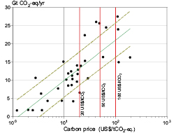
Figure 3.40: Permit price versus level of emission reduction – total economy in 2030 (the natural logarithm of the permit price is used for the x-axis). The uncertainty range indicated is the 68% interval.
Obviously, a considerable range of results is also found – this is a function of factors such as:
- Model uncertainties, including technology assumptions and inertia.
- Assumed baseline developments.
- The trajectory of the permit price prior to 2030.
The suggested relationship across the total is linear if permit prices are plotted on a logarithmic scale as shown in Figure 3.40 . In other words, the relationship between the two variables is logarithmic, which is a form that is consistent with the general form of marginal abatement curves reported in literature: increasing reduction levels for higher prices, but diminishing returns at higher prices as the reduction tends to reach a theoretical maximum. The figure not only shows the best-guess regression line, but also 68% confidence interval. The latter can be used to derive the 68 percentile interval of the reduction potential for the 20 and 100 US$/tCO2-eq price levels, which are 13.3 ± 4.6 GtCO2-eq/yr and 21.5 ± 4.7 GtCO2-eq/yr, respectively.
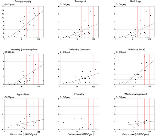
Figure 3.41: Permit price versus emission reduction level – several sectors in 2030 (vertical lines indicate levels at 20, 50 and 100 US$/tCO2).
Sectoral estimates
A more limited set of studies reported sectoral reduction levels. The same plot as Figure 3.40 has been made for the sectoral data (see Figure 3.41 ), again plotting the logarithm of the permit price against emission reduction levels. The data here are directly taken from Table 3.13 and Table 3.14 . As less data are available, the statistical analysis becomes less robust. Nevertheless, for most sectors, a similarly formed relationship was found across the set of studies as for the economy-wide potential (logarithmic relationship showing increasing reduction levels at relatively low prices, and a much slower increase at higher prices). As expected, in several sectors, the spread across models in the 2030 set is larger than in the economy-wide estimates.
In general, a relatively strong relationship is found in the sectors for energy supply, transport, and industrial energy consumption. The relationship between the price and emission reduction level is less clear in other sectors – and more-or-less absent for the limited reported data on the forestry sector. It should be noted here that definitions across studies may be less well-defined – and also, forest sector emissions may actually increase in mitigation scenarios as a result of net deforestation due to bio-energy production.
It should be noted that emission data (and thus also reduction levels) are reported on a ‘point of emission basis’ (emissions are reported for the sectors in which the emissions occur). For example, the efficiency improvements in end-use sectors for electricity lead to reductions in the energy supply sector. Likewise, using bio-energy leads to emission reductions in the end-use sectors, but at the same time (in some models) may lead to increases in emissions for forestry, due to associated land-use changes. The latter may explain differences in the way that data from top-down models are represented elsewhere in this report, as here (in most cases) only the emission changes from mitigation measures in the forestry sector itself are reported. It also explains why the potential in some of the end-use sectors is relatively small, as emission reductions from electricity savings are reported elsewhere.
Reported estimates
On the basis of the available data, the following ranges have been estimated for the reduction potential at a 20, 50 and 100 US$/tCO2-eq price ( Table 3.15 ). As estimates have been made independently, the total of the different sectors does not add up to the overall range (as expected, the sum of the sectors gives a slightly wider range).
Table 3.15: Reduction potential at various marginal prices, averages across different models (low and high indicate one standard deviation variation).
| 20 US$/tCO2-eq | 50 US$/tCO2-eq | 100 US$/tCO2-eq | ||||
|---|---|---|---|---|---|---|
| Low | High | Low | High | Low | High | |
| Energy supply | 3.9 | 9.7 | 6.7 | 12.4 | 8.7 | 14.5 |
| Transport | 0.1 | 1.6 | 0.5 | 1.9 | 0.8 | 2.5 |
| Buildings | 0.2 | 1.1 | 0.4 | 1.3 | 0.6 | 1.5 |
| Industry | 1.2 | 3.2 | 2.2 | 4.3 | 3.0 | 5.0 |
| Agriculture | 0.6 | 1.2 | 0.8 | 1.4 | 0.9 | 1.5 |
| Forestry | 0.2 | 0.8 | 0.2 | 0.8 | 0.2 | 0.8 |
| Waste | 0.7 | 0.9 | 0.8 | 1.0 | 0.9 | 1.1 |
| Overall1 | 8.7 | 17.9 | 13.7 | 22.6 | 16.8 | 26.2 |
The largest potential is found in energy supply – covering both the electricity sector and energy supply – with a relatively high capability of responding to permit prices. Relatively high reduction levels are also found for the industry sector. Relatively small reduction levels are reported for the forestry sector and the waste management sector.
REFERENCES
Aaheim, H.A., H. Asbjørn, J.S. Fuglestvedt, and O. Godal, 2006: Costs savings of a flexible multi-gas climate policy, The Energy Journal, Vol. Multi-Greenhouse gas Mitigation and Climate Policy, Special Issue No.3, pp. 485-502. [NPR]
Abramovitz, M., 1986: Catching-up, forging ahead, and falling behind. Journal of Economic History, 46(2), pp. 385-406. Clean
Aghion, P.P. and P. Howitt, 1998: Endogenous growth theory. MIT Press, Cambridge, 694 pp. [NPR]
Agrawala, S. (ed.), 2005: Bridge over troubled waters: Linking climate change and development. OECD Publishing, Paris, 154 pp. [NPR]
Ahammad, H., A. Matysek, B.S. Fisher, R. Curtotti, A. Gurney, G. Jakeman, E. Heyhoe, and D. Gunasekera, 2006: Economic impact of climate change policy: the role of technology and economic instruments. ABARE Research report 06.7, Canberra, 66 pp. <http://www.abareconomics.com/publications_html/climate/climate_06/cc_policy_nu.pdf>, accessed 1 June 2007. [NPR, SRC]
Ainsworth, E.A., S.P. Long, 2005: What have we learned from 15 years of free-air CO2 enrichment (FACE)? A meta-analytic review of the responses of photosynthesis, canopy properties and plant production to rising CO2. New Phytologist, 165, pp. 351-372. [NPR]
Akimoto, K., H. Kotsubo, T. Asami, X. Li, M. Uno, T. Tomoda, and T. Ohsumi, 2004: Evaluation of carbon dioxide sequestration in Japan with a mathematical model. Energy, 29(9-10), pp. 1537-1549. [MoS]
Alcamo, J., A. Bouwman, J. Edmonds, A. Grübler, T. Morita, and A. Sugandhy, 1995: An evaluation of the IPCC IS92 emission scenarios. In Climate change 1994, radiative forcing of climate change and an evaluation of the IPCC IS92 emission scenarios. Cambridge University Press, Cambridge, pp. 233-304. [NPR, MoS, ARC]
Alcamo, J. (ed.), 2002: Linkages between regional air pollution and climate change in Europe. Environmental Science & Policy, 5(4), pp. 255-365. Clean
Amann, M., 2002: Emission trends of anthropogenic air pollutants in the Northern Hemisphere. Air pollution as a climate forcing. Goddard Institute for Space Studies, Honolulu, Hawaii, 29 April – 3 May 2002. <http://www.giss.nasa.gov/meetings/pollution2002/d1_amann.html>, accessed 1 June 2007. [NPR, MoS, ARC]
Ambrosi, P., J.C. Hourcade, S. Hallegatte, F. Lecocq, P. Dumas, and M.H. Duong, 2003: Optimal control models and elicitation of attitudes towards climate damages. Environmental Modeling and Assessment, 8(3), pp. 133-147. [MoS, SRC]
Ambrosi, P., 2007: Mind the rate! Why the rate of global climate change matters, and how much. In Conference Volume of the 6th CESIfo Venice Summer Institute - David Bradford Memorial Conference on the Design of Climate Policy, R. Guesnerie and H. Tulkens (eds.), MIT Press, Cambridge MA. [NPR, SRC, 2007]
Andrae, M.O., 2001: The dark side of aerosols. Nature, 409(6821), pp. 671-672. [JoC]
Arnell, N.W., M.G.R. Cannell, M. Hulme, R.S. Kovats, J.F.B. Mitchell, R.J. Nicholls, M.L. Parry, M.T.J. Livermore and A. White, 2002: The Consequences of CO2 stabilisation for the impacts of climate change. Climatic Change, 53(4), pp. 413-446. [JoC]
Azar, C. and H. Dowlatabadi, 1999: A review of technical change in assessment of climate policy. Annual Review of Energy and the Environment, 24, pp. 513-544. Clean
Azar, C. and S.H. Schneider, 2001: Are uncertainties in climate and energy systems a justification for stronger near-term mitigation policies? Pew Center on Global Climate Change, 52 pp, <http://stephenschneider.stanford.edu/Publications/PDF_Papers/UncertaintiesInClimate.pdf>, accessed 1 June 2007. [NPR, PoC]
Azar, C. and K. Lindgren, 2003: Catastrophic events and stochastic cost-benefit analysis of climate change. An editorial comment. Climatic Change, 56(3), pp. 245-255. [JoC]
Azar, C., K. Lindgren, E. Larson, and K. Möllersten, 2006: Carbon capture and storage from fossil fuels and biomass - Costs and potential role in stabilizing the atmosphere. Climatic Change, 74(1-3), pp. 47-79. [JoC]
Babiker, M.H., J.M. Reilly, M. Mayer, R.S. Eckaus, I. Sue Wing, and R.C. Hyman, 2001: The emissions prediction and policy analysis (EPPA) model: revisions, sensitivities and comparisons of results. MIT, Cambridge MA. <http://web.mit.edu/globalchange/www/MITJPSPGC_Rpt71.pdf>, accessed 1 June 2007. [NPR, MoS, SRC]
Baranzini, A., M. Chesney, and J. Morisset, 2003: The impact of possible climate catastrophes on global warming policy. Energy Policy, 31(8), pp. 691-701. Clean
Barker, T., H. Pan, J. Köhler, R. Warren, S. Winne, 2006: Avoiding dangerous climate change by inducing technological progress: Scenarios using a large-scale econometric model. In Avoiding Dangerous Climate Change, H.J. Schellnhuber, W. Cramer, N. Nakicenovic, T. Wigley and G. Yohe (eds.), Cambridge University Press, Cambridge, pp. 361-373. [NPR, SRC]
Barro, R., 1991: Economic growth in a cross section of countries. Quarterly Journal of Economics, 106, pp. 407-443. Clean
Barro, R.J., and X. Sala-i-Martin, 1997: Technological diffusion, convergence, and growth. Journal of Economic Growth, 2(1), pp. 1-26. Clean
Baumol, W.J., 1986: Productivity growth, convergence, and welfare: what the long-run data show. American Economic Review, 76(5), pp. 1072-1085. Clean
Beierle, T.C. and J. Cayford, 2002: Democracy in practice: public participation in environmental decisions. Resources for the Future, Washington DC, 158 pp. [NPR, MoS]
Berndes, G., M. Hoogwijk, and R. van den Broek, 2003: The contribution of biomass in the future global energy system: a review of 17 studies. Biomass and Bioenergy, 25(1), pp. 1-28. [MoS, ARC]
Betts, R.A., 2000: Offset of the potential carbon sink from boreal forestation by decreases in surface albedo. Nature, 408(6809), pp. 187-190. [JoC]
Böhringer, C., A. Löschel, and T.F. Rutherford, 2006: Efficiency gains from “what”-flexibility in climate policy - An integrated CGE assessment, The Energy Journal, Vol. Multi-Greenhouse Gas Mitigation and Climate Policy, Special Issue, No.3, pp. 405-424. [NPR]
Bond, T.C., D.G. Streets, K.F. Yarber, S.M. Nelson, J.-H. Woo, and Z. Klimont, 2004: A technology-based global inventory of black and organic carbon emissions from combustion. Journal of Geophysical Research, 109(14), pp. D14203. [JoC]
Bosello, F. 2005: Adaptation and mitigation to global climate change: Conflicting strategies? Insights from an empirical integrated assessment exercise. University of Venice, 41 pp. <http://www.feem-web.it/ess05/files/Bosello.pdf>, accessed 1 June 2007. [NPR]
Bosello, F. and J. Zhang, 2005: Assessing climate change impacts: Agriculture. Fondazione Eni Enrico Mattei, Nota di lavoro 94.2005, Venice, 39 pp. <http://www.feem.it/NR/rdonlyres/8D8F51C4-EC35-4BC5-AA8F-67739BBC793C/1650/9405.pdf>, accessed 1 June 2007. [NPR]
Bouwman, A.F. and D.P. van Vuuren, 1999: Global assessment of acidification and eutrophication of natural ecosystems. Rijksinstituut voor Volksgezondheid en Milieu (RIVM), Report 402001 012, Bilthoven, 64 pp. <http://www.mnp.nl/bibliotheek/rapporten/402001012.pdf>, accessed 1 June 2007. [NPR, SRC]
Bradford, D.F., 2001: Time, money and tradeoffs. Nature, 410(6829), pp. 649-650. [JoC]
Brovkin, V., A. Ganopolski, M. Claussen, C. Kubatzki, and V. Petoukhov, 1999: Modelling climate response to historical land cover change. Global Ecology and Biogeography, 8(6), pp. 509-517. [MoS]
Brovkin, V., M. Claussen, E. Driesschaert, T. Fichefet, D. Kicklighter, M.F. Loutre, H. D. Matthews, N. Ramankutty, M. Schaeffer, and A. Sokolov, 2006: Biogeophysical effects of historical land cover changes simulated by six Earth system models of intermediate complexity. Climate Dynamics, 26(6), pp. 587-600. [MoS]
Bruinsma, J.E. (ed.), 2003: World agriculture: towards 2015/2030. An FAO perspective. Earthscan, London, 432 pp. [NPR]
Burrows, B., A. Mayne, and P. Newbury, 1991: Into the 21st century: a handbook for a sustainable future. Adamantine Press, Twickenham, 442 pp. [NPR, MoS]
Caldeira, K., A.K. Jain, and M.I. Hoffert, 2003: Climate sensitivity uncertainty and the need for energy without CO2 emission. Science, 299(5615), pp. 2052-2054. [JoC]
Carmichael, G.R., D.G. Streets, G. Calori, M. Amann, M.Z. Jacobson, J. Hansen, and H. Ueda, 2002: Changing trends in sulphur emissions in Asia: implications for acid deposition, air pollution, and climate. Environmental Science and Technology, 36(22), pp. 4707- 4713. [ARC]
Carpenter, S.R., P.L. Pingali, E.M. Bennet, M.B. Zurek (eds.), 2005: Ecosystems and Human Well-being: Scenarios, Vol.II, Millennium Ecosystem Assessment (MA), Island Press, Chicago, 561 pp. [NPR]
Carter, T.R., K. Jylhä, A. Perrels, S. Fronzek, and S. Kankaanpää, 2005: Alternative futures for considering adaptation to climate change in Finland. Finadapt Working Paper 2, Finnish Environment Institute, Helsinki, 42 pp. <http://www.ymparisto.fi/download.asp?contentid=44018&lan=en>, accessed 1 June 2007. [NPR, MoS]
Cassman, K.G., A. Dobermann, D.T. Walters, and H. Yang, 2003: Meeting cereal demand while protecting natural resources and improving environmental quality. Annual Review of Environmental Resources, 28, pp. 315-358. [ARC]
Castles, I. and D. Henderson, 2003a: Economics, emissions scenarios and the work of the IPCC. Energy and Environment, 14(4), pp. 415- 435. Clean
Castles, I. and D. Henderson, 2003b: The IPCC emission scenarios: an economic-statistical critique. Energy and Environment, 14(2-3), pp. 159-185. Clean
Central Planning Bureau, 1992: Scanning the future: a long-term scenario study of the world economy 1990-2015. SDU Publishers, The Hague, 246 pp. [NPR, MoS]
Chen, W., 2005: The costs of mitigating carbon emissions in China: Findings from China MARKAL-MACRO modeling. Energy Policy, 33(7), pp. 885-896. [MoS, ARC]
Cofala, J., M. Amann, Z. Klimont, and R. Mechler, 2006: Scenarios of world anthroprogenic emissions of air pollutants and methane up to 2030. IIASA Interim Report IR-06-023, International Institute of Applied Systems Analysis, Laxenburg. <http://www.iiasa.ac.at/rains/global_emiss/IR-06-023.pdf>, accessed 1 June 2007. [NPR, ARC]
Cohen, S.J., D. Neilsen, and R. Welbourn (eds.), 2004: Expanding the dialogue on climate change and water management on the Okanagan Basin, British Columbia. Natural Resources Canada, Ottawa, 241 pp. <http://www.ires.ubc.ca/downloads/publications/layout_Okanagan_final.pdf>, accessed 8 June 2007. [NPR]
Collins, W.J., D.E. Stevenson, C.E. Johnson, and R.G. Derwent, 2000: The European regional ozone distribution and its links with the global scale for the years 1992 and 2015. Atmospheric Environment, 34(2), pp. 255-267. Clean
Cooke, W.F. and J.J.N. Wilson, 1996: A global black carbon aerosol model. Journal of Geophysical Research, 101(14), pp. 19395-19409. [JoC, MoS]
Cooke, W.F., C. Liousse, H. Cachier, and J. Feichter, 1999: Construction of a 1º x 1º fossil fuel emission data set for carbonaceous aerosol and implementation and radiative impact in the ECHAM4 model. Journal of Geophysical Research, 104(D18), pp. 22137-22162. [JoC, MoS]
Corfee-Morlot, J. and N. Höhne, 2003: Climate change: long-term targets and short-term commitments. Global Environmental Change, 13(4), pp. 277-293. [JoC, ARC]
Corfee-Morlot, J., J. Smith, S. Agrawala, T. Franck, 2005: Long-term goals and post-2012 commitments: Where do we go from here with climate policy? Climate Policy, 5(3), pp. 251-272. [JoC]
Cox, P.M., R.A. Betts, C.B. Bunton, R.L.H. Essery, P.R. Rowntree, and J. Smith, 1999: The impact of new land surface physics on the GCM simulation of climate and climate sensitivity. Climate Dynamics, 15(3), pp. 183-203. [MoS]
Cox, P.M., R.A. Betts, C.D. Jones, S.A. Spall, and I.J. Totterdell, 2000: Acceleration of global warming due to carbon-cycle feedbacks in a coupled climate model. Nature, 408(6809), pp. 184-187. [JoC, MoS]
Cramer, W., A. Bondeau, S. Schaphoff, W. Lucht, B.E. Smith, and S. Sitch, 2004: Tropical forests and the global carbon cycle: impacts of atmospheric carbon dioxide climate change and rate of deforestations. Philosophical Transactions of the Royal Society of London Series B, 359(1443), pp. 331-343. Clean
Criqui, P., P. Russ, and D. Debye, 2006: Impacts of multi-gas strategies for greenhouse gas emission abatement: Insights from a partial equilibrium model. The Energy Journal, Vol. Multi-gas Mitigation and Climate Policy, Special Issue No.3, pp. 251-274. [NPR]
De la Chesnaye, F.C. and J.P. Weyant (eds.), 2006: Multi-gas mitigation and climate policy. The Energy Journal, Special Issue No.3, 520 pp. [SRC]
De la Chesnaye, F.C., C. Delhotal, B. DeAngelo, D. Ottinger-Schaefer, and D. Godwin, 2007: Past, present, and future of non-CO2 gas mitigation analysis. In Human-Induced Climate Change: An Interdisciplinary Assessment. M. Schlesinger, H. Kheshgi, J. Smith, F. de la Chesnaye, J.M. Reilly, T. Wilson, C. Kolstad (eds.), Cambridge University Press, Cambridge. [NPR, MoS, SRC, 2007]
Den Elzen, M.G.J. and M. Meinshausen, 2006: Multi-gas emission pathways for meeting the EU 2 C climate target. In Avoiding Dangerous Climate Change. H.J. Schellnhuber, W. Cramer, N. Nakicenovic, T. Wigley, and G. Yohe (eds.), Cambridge University Press, Cambridge. [NPR, ARC]
Den Elzen, M.G.J., M. Meinshausen, and D.P. Van Vuuren, 2006: Multi-gas emission envelopes to meet greenhouse gas concentration targets: Costs versus certainty of limiting temperature increase. In Stabilizing greenhouse gas concentrations at low levels, D.P. van Vuuren, M.G.J. Den Elzen, P.L. Lucas, B. Eickhout, B.J. Strengers, B. Van Ruijven, M.M. Berk, H.J.M. De Vries, S.J. Wonink, R. Van den Houdt, R. Oostenrijk, M. Hoogwijk, M. Meinshausen, Netherlands Environmental Assessment Agency (MNP), Bilthoven, 273 pp. [NPR, SRC]
Deutscher Bundestag, 2002: Enquete commission on sustainable energy supply against the background of globalisation and liberalisation: summary of the final report. Berlin. 80 pp. <http://www.bundestag.de/parlament/gremien/kommissionen/archiv14/ener/schlussbericht/engl.pdf>, accessed 1 June 2007. [NPR]
Dixon, P.B. and M.T. Rimmer, 2005: Analysing convergence with a multi-country computable general equilibrium model: PPP versus MER. Proceedings of 8th Annual Conference on Global Economic Analysis, Lübeck. <https://www.gtap.agecon.purdue.edu/resources/download/2254.pdf>, accessed 1 June 2007. [NPR, MoS]
Downing, T., D. Anthoff, R. Butterfield, M. Ceronsky, M. Grubb, J. Guo, C. Hepburn, C. Hope, A. Hunt, A. Li, A. Markandya, S. Moss, A. Nyong, R.S.J. Tol, and P. Watkiss. 2005. Social cost of carbon: a closer look at uncertainty. Department for Environment, Food and Rural Affairs, London, 95 pp. <http://www.defra.gov.uk/environment/climatechange/research/carboncost/pdf/sei-scc-report.pdf>, accessed 1 June 2007. [NPR, ARC]
Douglas, M. and A. Wildavsky, 1982: Risk and culture: an essay on the selection of technological and environmental damages. University of California Press, Berkeley. [NPR]
DTI, 2003: Energy White Paper: Our energy future - creating a low carbon economy. Department of Trade and Industry, London, 142 pp. <http://www.dti.gov.uk/files/file10719.pdf>, accessed 1 June 2007. [NPR, MoS]
Dumas, P. and M. Ha-Duong, 2005: An abrupt stochastic damage function to analyse climate policy benefits: essays on integrated assessment. In The Coupling of climate and economic dynamics: essays on integrated assessment. A. Haurie and L. Viguier (eds.), Springer Netherlands, pp. 97-111. [NPR]
Edenhofer, O., K. Lessmann, C. Kemfert, M. Grubb, J. Köhler, 2006: Induced technological change: Exploring its implications for the economics of atmospheric stabilization; Synthesis report from the innovation modeling comparison project. The Energy Journal, Vol. Endogenous Technological Change and the Economics of Atmospheric Stabilisation, Special Issue No.1, pp. 57-108. [NPR, ARC]
Edmonds, J.A., 2004: Technology options for a long-term mitigation response to climate change. 2004 Earth Technologies Forum, 13 April 2004, Pacific Northwest National Laboratory, Washington DC. [NPR, ARC]
Edmonds, J., J. Clarke, J. Dooley, S.H. Kim, and S.J. Smith, 2004a: Stabilization of CO2 in a B2 world: insights on the roles of carbon capture and disposal, hydrogen, and transportation technologies. Energy Economics, 26(4), pp. 517-537. [ARC]
Edmonds, J.A., J. Clarke, J. Dooley, S.H. Kim, S.J. Smith, 2004b: Modeling greenhouse gas energy technology responses to climate change. Energy, 29(9-10), pp. 1529-1536. [MoS, ARC]
Edmonds, J. and L. Clarke, 2005: Endogeneous technological change in long-term emissions and stabilization scenarios. IPCC Expert Meeting on Emissions Scenarios, 12 - 14 January 2005, Washington DC. [NPR, ARC]
Ehrlich, P.R. and J.P. Holdren, 1971: Impact of population growth. Science, 171(3977), pp. 1212-1217. [JoC]
European Commission, 2003: World energy, technology and climate policy outlook 2030 (WETO). EUR 20366, Office of Official Publications of European Communities, Luxembourg. <http://ec.europa.eu/research/energy/pdf/weto_final_report.pdf>, accessed 1 June 2007. [NPR]
Fagerberg, J., 1995: User-producer interaction, learning and competitive advantage. Cambridge Journal of Economics, 19(1), pp. 243-256. Clean
Fagerberg, J. and M. Godinho, 2005: Innovation and catching-up. In The Oxford Handbook of Innovation, J. Fagerberg, D.C. Mowery, R.R. Nelson (eds.), Oxford University Press, Oxford, pp. 514-542. [NPR]
Fawcett, A.A. and R.D. Sands, 2006: Non-CO2 greenhouse gases in the second generation model. The Energy Journal, Vol. Multi-Greenhouse Gas Mitigation and Climate Policy. Special Issue No.3, pp. 305-322. [MoS]
Fischedick, M. and J. Nitsch, 2002 (eds.): Long-term scenarios for a sustainable energy future in Germany. Wuppertal Institute for Climate, Environment, Energy; Wissenschaftszentrum Nordrhein-Westfalen, Wuppertal. <http://archive.greenpeace.org.au/climate/pdfs/Wuppertal_report.pdf>, accessed 1 June 2007. [NPR, 2007]
Fischedick, M., J. Nitsch, and S. Ramesohl, 2005: The role of hydrogen for the long-term development of sustainable energy systems - a case study for Germany. Solar Energy, 78(5), pp. 678-686. Clean
Fischer, G. and L. Schrattenholzer, 2001: Global bioenergy potentials through 2050. Biomass and Bioenergy, 20(3), pp. 151-159. Clean
Fisher, B.S., G. Jakeman, H.M. Pant, M. Schwoon, R.S.J. Tol, 2006: CHIMP: A simple population model for use in integrated assessment of global environmental change. The Integrated Assessment Journal, 6(3), pp. 1-33. [MoS, SRC]
Fankhauser, S. and R.S.J. Tol, 2005: On climate change and economic growth. Resource and Energy Economics, 27(1), pp. 1-17. [JoC]
Friedlingstein, P., P. Bopp, P. Ciais, J.-L. Dufresne, L. Fairhead, H. LeTreut, P. Monfray, and J. Orr, 2001: Positive feedback between future climate change and the carbon cycle. Geophysical Research Letters, 28(8), pp. 1543-1546. [MoS]
Füssel, H.-M. and J.G. van Minnen, 2001: Climate impact response functions for terrestrial ecosystems. The Integrated Assessment Journal, 2, pp. 183-197. Clean
Fuglestvedt, J.S., T.K. Berntsen, O. Godal, R. Sausen, K.P. Shine, T. Skodvin, 2003: Metrics of climate change: Assessing radiative forcing and emission indices. Climatic Change, 58(3), pp. 267-331. [JoC, MoS]
Fujino, J., R. Nair, M. Kainuma, T. Masui, and Y. Matsuoka, 2006: Multi-gas mitigation analysis on stabilization scenarios using AIM global model. The Energy Journal, Vol. Multi-Greenhouse Gas Mitigation and Climate Policy, Special Issue No.3, pp. 343-354. [NPR, SRC]
GCI, 2005: GCI Briefing: Contraction & Convergence. <http://www.gci.org.uk/briefings/ICE.pdf> accessed April 2006. [NPR]
Gallopin, G., A. Hammond, P. Raskin, and R. Swart, 1997: Branch points: global scenarios and human choice: a resource paper of the Global Scenario Group. Stockholm Environment Institute, Stockholm, 55 pp. <http://www.tellus.org/seib/publications/branchpt.pdf>, accessed 1 June 2007. [NPR, ARC]
Georgescu-Roegen, 1971: The Entropy Law and the Economic Process. Harvard University Press, Cambridge MA, 476 pp. [NPR]
Gitz, V. and P. Ciais, 2003: Amplifying effects of land-use change on future atmospheric CO2 levels. Global Biogeochemical cycles, 17(1), pp. 24-39. [NPR, MoS]
Gitz, V. and P. Ciais, 2004: Future expansion of agriculture and pasture acts to amplify atmospheric CO2 in response to fossil fuel and land-use change emissions. Climate Change, 67(2-3), pp. 161-184. [MoS]
Glenn, J.C. and T.J. Gordon, 1997: 1997 State of the future: implications for actions today. American Council for the United Nations University, Washington DC, 202 pp. [NPR, MoS]
Godal, O., 2003: The IPCC’s assessment of multidisciplinary issues: The case of greenhouse gas indices. Climate Change, 58(3), pp. 243-249. Clean
Goklany, I.M., 2003: Relative contributions of global warming to various climate sensitive risks, and their implications for adaptation and mitigation. Energy and Environment, 14(6), pp. 797-822. Clean
Goulder, L.H., 2004: Induced technological change and climate policy. Pew Center on Global Climate Change, Washington DC, 47 pp. <http://www.pewclimate.org/docUploads/ITC%5FReport%5FF2%2Epdf>, accessed 1 June 2007. [NPR]
Gray, H.A. and G.R. Cass, 1998: Source contributions to atmospheric fine carbon particle concentrations. Atmospheric Environment, 32(22), pp. 3805-3825. Clean
Gritsevskyi, A. and N. Nakicenovic, 2000: Modeling uncertainty of induced technological change. Energy Policy, 28(13), pp. 907-921. [MoS, SRC]
Grubb, M., O. Edenhofer, and C. Kemfert, 2005: Technological change and the innovation modeling comparison project. IPCC Expert Meeting on Emissions Scenarios, 12 - 14 January 2005, Washington DC. [NPR, MoS, ARC]
Grübler, A., 2002: Trends in global emissions: Carbon, sulphur and nitrogen, Encyclopedia of Global Environmental Change, 3, pp. 35-53. [ARC]
Grübler, A., N. Nakicenovic, and W.D. Nordhaus (eds.), 2002: Technological change and the environment. Resources for the Future Press, Washington DC, 407 pp. [NPR, MoS, SRC]
Grübler, A., N. Nakicenovic, J. Alcamo, G. Davis, J. Fenhann, B. Hare, S. Mori, B. Pepper, H. Pitcher, K. Riahi, H.H. Rogner, E.L. La Rovere, A. Sankovski, M. Schlesinger, R.P. Shukla, R. Swart, N. Victor, and T.Y. Jung, 2004: Emissions scenarios: a final response. Energy and Environment, 15(1), pp. 11-24. [SRC]
Grübler, A., B. O’Neill, K. Riahi, V. Chirkov, A. Goujon, P. Kolp, I. Prommer, S. Scherbov, and E. Slentoe, 2006: Regional, national, and spatially explicit scenarios of demographic and economic change based on SRES. Technological Forecasting and Social Change, Special Issue, 74(8–9). doi:10.1016/j.techfore.2006.05.023. [NPR, SRC]
GTSP, 2001: Global Energy Technology Strategy: Addressing Climate Change, 60 pp. <http://www.pnl.gov/gtsp/docs/infind/cover.pdf>, accessed 1 June 2007. [NPR]
Hall, D.C. and R.J. Behl, 2006: Integrating economic analysis and the science of climate instability. Ecological Economics, 57(3), pp. 442-465. Clean
Halloy, S.R.P. and J.A. Lockwood, 2005: Ethical implications of the laws of pattern abundance distribution. Emergence: Complexity and Organization, 7(2), pp. 41-53. [NPR]
Halsnaes, K., 2002: A review of the literature on climate change and sustainable development. In Climate change and sustainable development: prospects for developing countries. A. Markandya and Kirsten Halsnaes (eds.), Earthscan Publications, London, pp. 272. [NPR, ARC]
Hanaoka, T., R. Kawase, M. Kainuma, Y. Matsuoka, H. Ishii, and K. Oka, 2006: Greenhouse gas emissions scenarios database and regional mitigation analysis. CGER-D038-2006, National Institute for Environmental Studies, Tsukuba, 106 pp. <http://www-cger.nies.go.jp/publication/D038/all_D038.pdf>, accessed 1 June 2007. [NPR, SRC]
Hansen, J., M. Sato, R. Ruedy, A. Lacis, and V. Oinas, 2000: Global warming in the twenty-first century: an alternative scenario. Proceedings of the National Academy of Sciences of the United States of America, 97(18), pp. 9875-9880. [JoC]
Hanson, D.A., I. Mintzer, J.A. Laitner, and J.A. Leonard, 2004: Engines of growth: energy challenges, opportunities and uncertainties in the 21st century. Argonne National Laboratory, Argonne, IL, 59 pp. <http://www.ari.vt.edu/hydrogen/Resources/BackDoc/Doc/engines_growth.pdf>, accessed 1 June 2007. [NPR]
Hare, B. and M. Meinshausen, 2006: How much warming are we committed to and how much can be avoided? Climatic Change, 75(1-2), pp. 111-149. [JoC, ARC]
Harvey, L.D.D., 2004: Declining temporal effectiveness of carbon sequestration: implications for compliance with the United Nations Framework Convention on Climate Change. Climatic Change, 63(3), pp. 259-290. [JoC]
Harvey, L.D.D., 2006: Uncertainties in global warming science and near-term emission policies, Climate Policy, 6(5), pp. 573–584. [JoC]
Hayhoe, K., D. Cayan, C.B. Field, P.C. Frumhoff, E.P. Maurer, N.L. Miller, S.C. Moser, S.H. Schneider, K.N. Cahill, E.E. Cleland, L. Dale, R. Drapek, R.M. Hanemann, L.S. Kalkstein, J. Lenihan, C.K. Lunch, R.P. Neilson, S.C. Sheridan, and J.H. Verville, 2004: Emissions pathways, climate change, and impacts on California. Proceedings of the National Academy of Sciences of the United States of America, 101(34), pp. 12422-12427. [PoC, JoC, ARC]
Henderson, D., 2005: The treatment of economic issues by the Intergovernmental Panel on Climate Change. Energy & Environment, 16(2), pp. 321-326. Clean
Herzog, H., K. Smekens, P. Dadhich, J. Dooley, Y. Fujii, O. Hohmayer, K. Riahi, 2005: Cost and economic potential. In: IPCC Special Report on Carbon Dioxide Capture and Storage. Intergovernmental Panel on Climate Change, Cambridge University Press, Cambridge, pp. 339-362. [NPR, SRC]
Hijioka, Y, T. Masui, K. Takahashi, Y. Matsuoka, and H. Harasawa, 2006: Development of a support tool for greenhouse gas emissions control policy to help mitigate the impact of global warming. Environmental Economics and Policy Studies, 7(3), pp. 331-345. Clean
Holdren, J.P., 2000: Environmental degradation: population, affluence, technology, and sociopolitical factors. Environment, 42(6), pp. 4-5. Clean
Holtsmark, B.J. and K.H. Alfsen, 2004a: PPP correction of the IPCC emission scenarios - does it matter? Climatic Change, 68(1-2), pp. 11-19. [JoC, SRC]
Holtsmark, B.J. and K.H. Alfsen, 2004b: The use of PPP or MER in the construction of emission scenarios is more than a question of ‘metrics’. Climate Policy, 4(2), pp. 205-216. [JoC, SRC]
Hoogwijk, M., A. Faaij, B. Eickhout, B. de Vries and W. Turkenburg, 2005: Potential of biomass energy out to 2100, for four IPCC SRES land-use scenarios. Biomass and Bioenergy, 29(4), pp. 225-257. [SRC]
Hope, C., 2006: The Marginal Impact of CO2 from PAGE 2002: an Integrated Assessment Model Incorporating the IPCC’s Five Reasons for Concern. The Integrated Assessment Journal, 6(1), pp. 19-56. [MoS]
Houghton, R.A., 2003: Revised estimates of the annual net flux of carbon to the atmosphere from changes in land use and land management 1850-2000. Tellus, Serie B: Chemical and Physical Meteorology, 55b(2), pp. 378-390. [NPR, MoS]
Hourcade, J.-C. and P. Shukla, 2001: Global, regional and national costs and ancillary benefits of mitigation. In Climate change 2001: Mitigation. Contribution of Working Group III to the Third Assessment Report of the Intergovernmental Panel on Climate Change. Cambridge University Press, Cambridge MA, pp. 702. [NPR, ARC]
House, J.I., I.C. Prentice, and C. Le Quere, 2002: Maximum impacts of future reforestation or deforestation on atmospheric CO2. Global Change Biology, 8(11), pp. 1047-1052. [MoS]
Howarth, R.B., 2003: Catastrophic outcomes in the economics of climate change. An editorial comment. Climatic Change, 56(3), pp. 257-263. [JoC]
IEA, 2002: World Energy Outlook 2002. International Energy Agency, Paris, 530 pp. [NPR]
IEA, 2004: World Energy Outlook 2004. International Energy Agency, Paris, 570 pp. [NPR]
IPCC, 1996a: Climate Change 1995: impacts, adaptations and mitigation of climate change: scientific-technical analysis. Contribution of Working Group II to the Second Assessment Report of the IPCC. R.T. Watson, M.C. Zinyowera, R.H. Moss [eds], Intergovernmental Panel on Climate Change, Cambridge University Press, Cambridge. [NPR]
IPCC, 1996b: Climate Change 1995: economic and social dimensions of climate change. Contribution of Working Group III to the Second Assessment Report of the IPCC. J.B. Bruce, H. Lee, E.F. Haites [eds], Intergovernmental Panel on Climate Change, Cambridge University Press, Cambridge. [NPR]
IPCC, 1997: Revised 1996 IPCC Guidelines for National Greenhouse Inventories. Intergovernmental Panel on Climate Change, IPCC/OECD/IEA, Paris, France. [NPR]
IPCC, 2000: Land use, land-use change and forestry. A special report of the IPCC. Intergovernmental Panel on Climate Change, Cambridge University Press, Cambridge UK, 377 pp. [NPR]
IPCC, 2001a: Climate change 2001: Mitigation. Contribution of Working Group III to the Third Assessment Report of the IPCC. Intergovernmental Panel on Climate Change, Cambridge University Press, Cambridge, UK, 702 pp. [NPR]
IPCC, 2001b: Climate Change 2001: The Scientific Basis. Contribution of Working Group I to the Third Assessment Report of the IPCC. Intergovernmental Panel on Climate Change, Intergovernmental Panel on Climate Change, Cambridge University Press, UK, 944 pp. [NPR]
IPCC, 2007a: Climate Change 2007: The Physical Science Basis. Contribution of Working Group I to the Fourth Assessment Report of the Intergovernmental Panel on Climate Change [Solomon, S., D. Qin, M. Manning, Z. Chen, M. Marquis, K.B.M.Tignor and H.L. Miller (eds.)]. Cambridge University Press, Cambridge, United Kingdom and New York, NY, USA, 996 pp. [NPR, 2007]
IPCC, 2007b: Climate Change 2007: Impacts, Adaptation and Vulnerability. Contribution of Working Group II to the Fourth Assessment Report of the Intergovernmental Panel on Climate Change [Parry, M.L., O.F. Canziani, J.P. Palutikof, P.J. van der Linden, C.E. Hanson (eds.)]. Cambridge University Press, Cambridge, United Kingdom and New York, NY, USA. [NPR, 2007]
Izrael, Y.A. and S.M. Semenov, 2005: Calculations of a change in CO2 concentration in the atmosphere for some stabilization scenarios of global emissions using a model of minimal complexity. Russian Meteorology and Hydrology, 1, pp. 1-8. [MoS]
Jacobson, M.Z., 2001: Strong radiative heating due to the mixing state of black carbon in atmospheric aerosols. Nature, 409(6821), pp. 695-697. [JoC]
Jacoby, H.D., 2004: Informing climate policy given incommensurable benefits estimates. Global Environment Change, 14(3), pp. 287-297. [JoC, MoS]
Jakeman, G. and B.S. Fisher, 2006: Benefits of multi-gas mitigation: An application of the global trade and environment model (GTEM). The Energy Journal, Multi-Greenhouse Gas Mitigation and Climate Policy, Special Issue No.3, pp. 323-342. [NPR, SRC]
JAIF, 2004: 2050 Nuclear Vision and Roadmap. Japan Atomic Industrial Forum, Inc, Tokyo. <http://www.jaif.or.jp/english/news/2005/0317vision.html>, accessed 1 June 2007. [NPR]
Japan LCS Project, 2005: Backcasting from 2050, Japan Low Carbon Society Scenarios Toward 2050. LCS Research Booklet No.1, National Institute for Environmental Studies, Tsukuba, 11 pp, <http://2050.nies.go.jp/material/lcs_booklet/lcs_booklet.html>, accessed 1 June 2007. [NPR]
Jiang, K. and H. Xiulian, 2003: Long-term GHG emissions scenarios for China. Second Conference on Climate Change, Beijing. [NPR, SRC]
Jiang, K., H. Xiulian, and S. Zhu, 2006: Multi-gas mitigation analysis by IPAC. The Energy Journal, Vol. Multi-Greenhouse Gas Mitigation and Climate Policy, Special Issue No.3, pp. 425-440. [NPR, SRC]
Johansson, D.J.A., U.M. Persson and C. Azar, 2006: The cost of using global warming potentials: Analysing the trade off between CO2, CH4 and N2O. Climatic Change, 77(3-4), pp. 291-309. [JoC]
Jones, C.I., 1997: Convergence revisited. Journal of Economic Growth, 2(2), pp. 131-153. Clean
Jung, T.Y., E.L. La Rovere, H. Gaj, P.R. Shukla, and D. Zhou, 2000: Structural changes in developing countries and their implication to energy-related CO2 emissions. Technological Forecasting and Social Change, 63(2-3), pp. 111-136. [SRC]
Junker, C. and C. Liousse, 2006: A Global Emission Inventory of Carbonaceous Aerosol from historic records of Fossil Fuel and Biofuel consumption for the Period 1860 - 1997, Atmospheric Chemistry and Physics Discussions, 6, pp. 4897–4927 Clean
Kahn, H. and A. Weiner, 1967: The year 2000: a framework for speculation on the next thirty-three years. Macmillan, New York, 431 pp. [NPR]
Kahn, H., W. Brown, and L. Martel, 1976: The next 200 years: a scenario for America and the World. Morrow, New York, 241 pp. [NPR]
Kaplan, R.D., 1994: The coming anarchy. The Atlantic Monthly, 272(2), pp. 44-76. Clean
Kawase, R., Y. Matsuoka, and J. Fujino, 2006: Decomposition analysis of CO2 emission in long-term climate stabilization scenarios. Energy Policy, 34(15), pp. 2113-2122. Clean
Keller, K., K. Tan, F.M.M. Morel, and D.F. Bradford, 2000: Preserving the ocean circulation: implications for climate policy. Climatic Change, 47(1-2), pp. 17-43. [JoC]
Keller, K., B.M. Bolker, and D.F. Bradford, 2004: Uncertain climate thresholds and economic optimal growth. Journal of Environmental Economics and Management, 48, pp. 723-741. Clean
Keller, K., G. Yohe, and M. Schlesinger, 2006: Managing the risks of climate thresholds: Uncertainties and information needs. Climatic Change, doi:10.1007/s10584-006-9114-6. <http://www.geosc.psu.edu/~kkeller/publications.html>, accessed 1 June 2007. [JoC]
Kelly, D.L., C.D. Kolstad, M.E. Schlesinger, and N.G. Andronova, 2000: Learning about climate sensitivity from the instrumental temperature record. <http://www.econ.ucsb.edu/papers/wp32-98.pdf>, accessed 1 June 2007. [NPR, ARC]
Kelly, D.L., C.D. Kolstad, and G.T. Mitchell, 2005: Adjustment costs from environmental change. Journal of Environmental Economics and Management, 50(3), pp. 468-495. [ARC]
Kemfert, C., 2002: Global economic implications of alternative climate policy strategies. Environmental Science and Policy, 5(5), pp. 367-384. Clean
Kemfert, C. and K. Schumacher, 2005: Costs of inaction and costs of action in climate protection: assessment of costs of inaction or delayed action of climate protection and climate change. Final Report: Project FKZ 904 41 362 for the Federal Ministry for the Environment, Berlin. <http://www.diw.de/deutsch/produkte/publikationen/diwkompakt/docs/diwkompakt_2005-013.pdf>, accessed 1 June 2007. [NPR]
Kemfert, C., 2006: An integrated assessment of economy, energy and climate. The model WIAGEM - A reply to comment by Roson and Tol. The Integrated Assessment Journal, 6(3), pp. 45-49. [MoS]
Kemfert, C., T.P. Truong, and T. Bruckner, 2006: Economic impact assessment of climate change - A multi-gas investigation with WIAGEM-GTAPEL-ICM. The Energy Journal, Multi-Greenhouse Gas Mitigation and Climate Policy, Special Issue No.3, pp. 441-460. [NPR]
Keppo, I., B. O’Neill, and K. Riahi, 2006: Probabilistic temperature change projections and energy system implications of greenhouse gas emission scenarios. Technological Forecasting and Social Change, Special Issue, 74(8–9), doi:10.1016/j.techfore.2006.05.024. [NPR, MoS, SRC]
Kheshgi, H.S. 2004: Evasion of CO2 injected into the ocean in the context of CO2 stabilization. Energy, 29(9-10), pp. 1479-1486. [ARC]
Kheshgi, H.S., S.J. Smith, and J.A. Edmonds, 2005: Emissions and atmospheric CO2 stabilization: Long-term limits and paths. Mitigation and Adaptation Strategies for Global Change, 10(2), pp. 213-220. [ARC]
Kinsman, F., 1990: Millennium: towards tomorrow’s society. W.H. Allen, London. [NPR]
Kokic, P., A. Heaney, L. Pechey, S. Crimp, and B.S. Fisher, 2005: Climate change: predicting the impacts on agriculture: a case study. Australian Commodities, 12(1), pp. 161-170. [MoS, SRC]
Köhler, J., M. Grubb, D. Popp and O. Edenhofer, 2006: The transition to endogenous technical change in climate-economy models: A technical overview to the innovation modeling comparison project. The Energy Journal, Endogenous Technological Change and the Economics of Atmospheric Stabilisation, Special Issue No. 1. [NPR, ARC]
Kupiainen, K. and Z. Klimont, 2004: Primary emissions of submicron and carbonaceous particles in Europe and the potential for their control. IR-04-079, International Institute for Applied Systems Analysis Interim Report, Laxenburg. <http://www.iiasa.ac.at/rains/reports/ir-04-079.pdf>, accessed 1 June 2007. [NPR]
Kurosawa, A., 2004: Carbon concentration target and technological choice. Energy Economics, 26(4), pp. 675-684. Clean
Kurosawa, A., 2006: Multi-gas mitigation: An economic analysis using GRAPE model. The Energy Journal, Vol. Multi-Greenhouse Gas Mitigation and Climate Policy, Special Issue No.3, pp. 275-288. [NPR]
Kypreos, S., 2006: Stabilizing global temperature change below thresholds; A Monte Carlo analyses with MERGE. Paul Scherrer Institut, Villigen, 28 pp. <http://eem.web.psi.ch/Publications/Books_Journals/2006_Kypreos_stabilizing_with_merge.pdf>, accessed 1 June 2007. [NPR, MoS]
La Rovere, E.L. and B.B. Americano, 2002: Domestic actions contributing to the mitigation of GHG emissions from power generation in Brazil. Climate Policy, 2(2-3), pp. 247-254. [JoC, SRC]
Lazarus, M., L. Greber, J. Hall, C. Bartels, S. Bernow, E. Hansen, P. Raskin, and D. Von Hippel, 1993: Towards a fossil free energy future: the next energy transition. Stockholm Environment Institute, Boston Center, Boston. Greenpeace International, Amsterdam. [NPR, MoS]
Leemans, R., B. Eickhout, B. Strengers, L. Bouwman, and M. Schaeffer, 2002: The consequences of uncertainties in land use, climate and vegetation responses on the terrestrial carbon. Science in China, 45(Supplement), pp. 126-141. [SRC]
Leggett, J., W.J. Pepper, and R.J. Swart , J. Edmonds, L.G. Meira Filho, I. Mintzer, M.X. Wang, and J. Watson, 1992: Emissions scenarios for IPCC: an update. In Climate change 1992: the supplementary report to the IPCC Scientific Assessment. Cambridge University Press, Cambridge. [NPR, ARC]
Lehtila, A., I. Savolainen, and S. Syri, 2005: The role of technology development in greenhouse gas emissions reduction: the case of Finland. Energy, 30(14), pp. 2738-2758. Clean
Lempert, R.J., M.E. Schlesinger, and J.K. Hammitt, 1994: The impact of potential abrupt climate changes on near-term policy changes. Climatic Change, 26(4), pp. 351-376. [JoC]
Levy, P.E., A.D. Friend, A. White, and M.G.R. Cannell, 2004: The influence of land use change on global-scale fluxes of carbon from terrestrial ecosystems. Climatic Change, 67(2-3), pp. 185-209. [JoC]
Liousse, C., J.E. Penner, C. Chuang, J.J. Walton, H. Eddleman, and H. Cachier, 1996: A global three-dimensional model study of carbonaceous aerosols. Journal of Geophysical Research, 101(14), pp. 19411-19432. [JoC, MoS]
Liousse, C., B. Guillaume, C. Junker, C. Michel, H. Cachier, B. Guinot, P. Criqui, S. Mima, and J.M. Gregoire, 2005: Management and impact on climate change (a french initiative). GICC report, Carbonaceous Aerosol Emission Inventories from 1860 to 2100, March. <http://medias.obs-mip.fr/gicc/interface/projet.php?4/01>, accessed 1 June 2007. [NPR]
Lutz, W. and W. Sanderson, 2001: The end of world population growth. Nature, 412(6846), pp. 543-545. [JoC]
Lutz, W., W.C. Sanderson, and S. Scherbov, 2004: The end of world population growth. In: The end of world population growth in the 21st century: New challenges for human capital formation and sustainable development. W. Lutz and W. Sandersen (eds.), Earthscan Publications, London, pp. 17-83. [NPR]
Maddison, D., 2001: The amenity value of global climate. Earthscan, London, 240 pp. [NPR]
Mankiw, N.G., D. Romer, and D.N. Weil, 1992: A contribution to the empirics of economic growth. Quarterly Journal of Economics, 107(2), pp. 407-437. Clean
Manne, A.S. and R.G. Richels, 2001: An alternative approach to establishing trade-offs among greenhouse gases. Nature, 410(6829), pp. 675-677. [JoC, SRC]
Manne, A. and R. Richels, 2003: Market exchange rates or purchasing power parity: does the choice make a difference in the climate debate? AEI-Brookings Joint Center for Regulatory Studies, Working Paper No. 03-11, 14 pp. <http://ssrn.com/abstract=449265>, accessed 1 June 2007. [NPR, SRC]
Manne, A. and R. Richels, 2004: The impact of learning-by-doing on the timing and costs of CO2 abatement. Energy Economics, 26(4), pp. 603-619. [SRC]
Manne, A.S. and R.G. Richels, 2006: The role of non-CO2 greenhouse gases and carbon sinks in meeting climate objectives. The Energy Journal, Vol. Multi-Greenhouse Gas Mitigation and Climate Policy, Special Issue No.3, pp. 393-404. [NPR, SRC]
Martins, J.O. and G. Nicoletti, 2005: Long-term economic growth projections: could they be made less arbitrary? IPCC Expert Meeting on Emissions Scenarios, 12 - 14 January 2005, Washington DC. [NPR, MoS]
Mastrandrea, M.D., and S.H. Schneider, 2001: Integrated assessment of abrupt climatic changes. Climate Policy, 1(4), pp. 433-449. [PoC, JoC, SRC]
Mastrandrea, M.D. and S.H. Schneider, 2004: Probabilistic integrated assessment of ‘dangerous’ climate change. Science, 304(5670), pp. 571-575. [PoC, JoC, SRC]
Masui, T., Y. Matsuoka, and M. Kainuma, 2006: Long-term CO2 emission reduction scenarios in Japan. Environmental Economics and Policy Studies, 7(3), pp. 347-366. [SRC]
Matthews, H.D., A.J. Weaver, M. Eby, and K.J. Meissner, 2003: Radiative forcing of climate by historical land cover change. Geophysical Research Letters, 30(2), pp. 1055-1059. [MoS]
Matthews, H.D., 2005: Decrease of emissions required to stabilize atmospheric CO2 due to positive carbon cycle-climate feedbacks. Geophysical Research Letters, 32, L21707. Clean
Mayerhofer, P., B. de Vries, M.G.J. den Elzen, D.P. van Vuuren, J. Onigkeit, M. Posch, and R. Guardans, 2002: Long-term, consistent scenarios of emissions, deposition and climate change in Europe. Environmental Science and Policy, 5(4), pp. 273-305. [SRC]
McGuire, A.D., S. Sitch, J.S. Clein, R. Dargaville, G. Esser, J. Foler, M. Heimann, F. Joos, J. Kaplan, D.W. Kicklighter, R.A. Meier, J.M. Melillo, B. Moore, I.C. Prentice, N. Ramankutty, T. Reichenau, A. Schloss, H. Tian, L.J. Williams, and U. Wittenberg, 2001: Carbon balance of the terrestrial biosphere in the twentieth century: analyses of CO2, climate and land use effects with four process-based ecosystem models. Global Biogeochemical Cycles, 15(1), pp. 183-206. [PoC, JoC, MoS]
McKibbin, W.J., D. Pearce, and A. Stegman, 2004a: Can the IPCC SRES be improved? Energy and Environment, 15(3), pp. 351-362. Clean
McKibbin, W.J., D. Pearce, and A. Stegman, 2004b: Long-run projections for climate change scenarios. Centre for Applied Macroeconomics Analysis Working Paper Series, Australian National University, Canberra, 71 pp. <http://cama.anu.edu.au/Working%20Papers/Papers/2004/McKibbinPaper12004.pdf>, accessed 1 June 2007. [NPR, MoS]
Meadows, D.H., D.L. Meadows, J. Randers, and W.W. Behrens, 1972: The limits to growth: a report for the club of Rome’s project on the predicament of mankind. Universe Books, New York. [NPR]
Meehl, G.A., W.M. Washington, W.D. Collins, J.M. Arblaster, A. Hu, L.E. Buja, W.G. Strand, and H. Teng, 2005: How much more global warming and sea level rise? Science, 307(5716), pp. 1769-1772. [JoC]
Meehl, G. A., T. F. Stocker, W. D. Collins, P. Friedlingstein, A. T. Gaye, J. M. Gregory, A. Kitoh, R. Knutti, J. M. Murphy, A. Noda, S. C. B. Raper, I. G. Watterson, A. J. Weaver, Z.-C. Zhao, 2007: Global Climate Projections. In Climate Change 2007: The Physical Science Basis. Contribution of Working Group I to the Fourth Assessment Report of the Intergovernmental Panel on Climate Change, S. Solomon, D. Qin, M. Manning, Z. Chen, M. Marquis, K. B. Averyt, M. Tignor, and H. L. Miller (eds.), Cambridge University Press, Cambridge, UK and New York, NY, USA. [NPR, MoS, 2007]
Meier, G.M., 2001: The old generation of development economists and the new. In Frontiers of development economics. The Future in perspective. G.M. Meier and J.M. Stiglitz (eds.), Oxford University Press, New York. [NPR, MoS]
Meinshausen, M., 2006: What does a 2 °C Target mean for greenhouse gas concentrations? A brief analysis based on multi-gas emission pathways and several climate sensitivity uncertainty estimates. In Avoiding Dangerous Climate Change. H.J. Schellnhuber, W. Cramer, N. Nakicenovic, T. Wigley, and G. Yohe (eds.), Cambridge University Press, Cambridge. [NPR, MoS]
Meinshausen, M., B. Hare, T.M.M. Wigley, D. van Vuuren, M.G.J. den Elzen, and R. Swart, 2006: Multi-gas emissions pathways to meet climate targets. Climatic Change, 75(1-2), pp. 151-194. [JoC, SRC]
Mendelsohn, R., W. Morrison, M.E. Schlesinger, and N.G. Andronova, 2000: Country-specific market impacts of climate change. Climatic Change, 45(3-4), pp. 553. [JoC]
Mendelsohn, R. and L. Williams, 2004: Comparing forecasts of the global impacts of climate change. Mitigation and Adaptation Strategies for Global Change, 9(4), pp. 315-333. [MoS]
Mesarovic, M.D. and E. Pestel, 1974: Mankind at the turning point: the second report to the Club of Rome. Dutton, New York, 210 pp. [NPR]
Metz, B. and D. P. Van Vuuren, 2006: How, and at what costs, can low-level stabilisation be achieved? - An overview. In Avoiding Dangerous Climate Change. H.J. Schellnhuber, W. Cramer, N. Nakicenovic, T. Wigley, and G. Yohe (eds.), Cambridge University Press, Cambridge, UK. [NPR, SRC]
METI, 2005: Strategic Technology Roadmap (Energy Sector) - Energy Technology Vision 2100-. Ministry of Economy, Trade and Industry, The Institute of Applied Energy, Tokyo, 96 pp. <http://www.iae.or.jp/2100/main.pdf>, accessed 1 June 2007. [NPR]
MIES, 2004: Reducing CO2 emissions fourfold in France by 2050: introduction to the debate. La Mission Interministérielle de l’Effet de Serre, Paris, 40 pp. <http://www.climnet.org/pubs/1004_France_Factor%204.pdf>, accessed 1 June 2007. [NPR]
Mintzer, I., J.A. Leonard, and P. Schwartz, 2003: U.S. energy scenarios for the 21st century. Pew Center on Global Climate Change, Arlington, 88 pp. <http://www.pewclimate.org/docUploads/EnergyScenarios.pdf>, accessed 1 June 2007. [NPR]
Morgenstern, 2000: Baseline issues in the estimation of ancillary benefits of greenhouse gas mitigation policies, Ancillary benefits and costs of greenhouse gas mitigation. OECD Proceedings of an IPCC Co-sponsored Workshop, 27-29 March 2000, in Washington DC, OECD Publishing, Paris, pp. 95-122. [NPR, MoS]
Mori, S., 2003: Issues on global warming, energy and food from the long-term point of view. Journal of the Japan Institute of Energy, 82(1), pp. 25-30. Clean
Morita, T. and H.-C. Lee, 1998: Appendix: IPCC Emissions Scenarios Database, Mitigation and Adaptation Strategies for Global Change, 3, pp. 121-131. [ARC]
Morita, T., J. Robinson, A. Adegbulugbe, J. Alcamo, D. Herbert, E. Lebre La Rovere, N. Nakicenovic, H. Pitcher, P. Raskin, K. Riahi, A. Sankovski, V. Sololov, B. de Vries and D. Dadi, 2001: Greenhouse gas emission mitigation scenarios and implications. In Climate change 2001: Mitigation, Report of Working Group III of the IPCC. Cambridge University Press, Cambridge, pp. 115-166. [NPR, SRC]
Nair, R., P.R. Shukla, M. Kapshe, A. Garg, and A. Rana, 2003: Analysis of long-term energy and carbon emission scenarios for India. Mitigation and Adaptation Strategies for Global Change, 8(1), pp. 53-69. [SRC]
Nakicenovic, N., 1996: Freeing energy from carbon. Daedalus, 125(3), pp. 95-112. [SRC]
Nakicenovic, N., J. Alcamo, G. Davis, B. de Vries, J. Fenham, S. Gaffin, K. Gregory, A. Grübler, T.-Y. Jung, T. Kram, E.L. La Rovere, L. Michaelis, S. Mori, T. Morita, W. Pepper, H. Pitcher, L. Price, K. Riahi, A. Reohrl, H.H. Rogner, A. Sankovski, M. Schlesinger, P. Shukla, S. Smith, R. Swart, S. van Rooijen, N. Victor, and Z. Dadi, 2000: Special report on emissions scenarios. Working Group III, Intergovernmental Panel on Climate Change (IPCC). Cambridge University Press, Cambridge, 595 pp. [NPR, SRC]
Nakicenovic, N. and K. Riahi, 2003: Model runs with MESSAGE in the context of the further development of the Kyoto-Protocol. Wissenschaftlicher Beirat der Bundesregierung Globale Umweltveränderungen, Berlin, 54 pp. <http://www.wbgu.de/wbgu_sn2003_ex03.pdf>, accessed 1 June 2007. [NPR, MoS, SRC]
Nakicenovic, N., A. Grübler, S. Gaffin, T.T. Jung, T. Kram, T. Morita, H. Pitcher, K. Riahi, M. Schlesinger, P.R. Shukla, D. van Vuuren, G. Davis, L. Michaelis, R. Swart, and N. Victor, 2003: IPCC SRES revisited: a response. Energy and Environment, 14(2-3), pp. 187-214. [SRC]
Nakicenovic, N., J. McGalde, S. Ma, J. Alcamo, E. Bennett, W. Cramer, J. Robinson, F.L. Toth, M. Zurek, 2005: Lessons learned for scenario analysis. In Ecosystems and Human Well-being: Scenarios. Carpenter, S.R., P.L. Pingali, E.M. Bennet, M.B. Zurek (eds.), Vol.II, Millennium Ecosystem Assessment (MA), Island Press, Chicago, pp. 449-468. [NPR, SRC]
Nakicenovic, N., P. Kolp, K. Riahi, M. Kainuma, T. Hanaoka, 2006: Assessment of emissions scenarios revisited. Environmental Economics and Policy Studies, 7(3), pp. 137-173. [SRC]
Newell, R.G., A.B. Jaffe, and R.N. Stavins, 1999: The induced innovation hypothesis and energy-saving technological change. Quarterly Journal of Economics, 114(3), pp. 941-975. Clean
Nicholls, R.J., S.E. Hansen, J.A. Lowe, D.A.Vaughan, T. Lenton, A. Ganopolski, R.S.J. Tol, and A.T. Vafeidis, 2006: Metrics for assessing the economic benefits of climate change policies: sea level rise, Organisation for Economic Co-operation and Development, ENV/EPOC/GSP(2006)3/FINAL, OECD Publishing, Paris, pp. 125. <http://www.oecd.org/dataoecd/19/63/37320819.pdf>, accessed 1 June 2007. [NPR]
Nordhaus, W.D. and J. Boyer, 2000: Warming the world: economic models of global warming. MIT Press, Cambridge MA, 244 pp. [NPR, MoS]
Nordhaus, W.D., 2005: Should modelers use purchasing power parity or market exchange rates in global modelling systems. IPCC Seminar on Emission Scenarios, Intergovernmental Panel on Climate Change (IPCC), 12 - 14 January 2005, Washington DC. [NPR, MoS]
Nordhaus, W.D., 2006a: Geography and macroeconomics: New data and new findings. Proceedings of the National Academy of Sciences of the United States of America, 103(10), pp. 3510-3517. [JoC]
Nordhaus, W.D., 2006b: The “Stern” review on the economics of climate change. National Bureau of Economic Research, Working Paper No. 12741, pp. 10. <http://ssrn.com/abstract=948654>, accessed 1 June 2007. [NPR]
NRCan, 2000: Energy Technology Futures. 2050 Study: Greening the pump. National Resources Canada, Ottowa. [NPR, MoS]
OECD, 2000: Ancillary benefits and costs of greenhouse gas mitigation. Organisation for Economic Co-operation and Development Proceedings of an IPCC co-sponsored workshop in Washington DC, 27-29 March 2000, OECD Publishing, Paris. [NPR]
OECD, 2003: Organisation for Economic Co-operation and Development Workshop on the benefits of climate policy: improving information for policy makers. 12-13 December 2002, OECD Publishing, Paris. [NPR]
Olivier, J.G.J., A.F. Bouwman, K.W. Van der Hoek, and J.J.M. Berdowski, 1998: Global air emission inventories for anthropogenic sources of NOx, NH3 and N2O in 1990. Environmental Pollution, 102(Supplement 1), pp. 135-148. [NPR, ARC]
Olivier, J.G.J. and J.J.M. Berdowski, 2001: Global emissions sources and sinks. In The Climate System. J. Berdowski, R. Guicherit and B.J. Heij (eds.), A.A. Balkema/Swets & Zeitlinger, Lisse, pp. 33-78. [NPR, ARC]
O’Neill, B.C. and M. Oppenheimer, 2002: Dangerous climate impacts and the Kyoto Protocol, Science, 296(5575), pp. 1971-1972. [JoC, SRC]
O’Neill, B.C., 2003; Economics, natural science, and the costs of Global Warming Potentials. Climatic Change, 58(3), pp. 251-260. [JoC, SRC]
O’Neill, B.C., 2004: Conditional probabilistic population projections: an application to climate change. International statistical review, 72(2), pp. 167-184. [NPR, MoS, SRC]
O’Neill, B.C. and M. Oppenheimer, 2004: Climate change impacts sensitive to the concentration stabilization path. Proceedings of the National Academy of Science of the United States of Amercia, 101(47), pp. 16411-16416. [SRC]
Ostrom, E., 1990: Governing the commons: The evolution of institutions for collective action. Cambridge University Press, Cambridge, 298 pp. [NPR]
Ostrom, E., T. Dietz, N. Dolsak, P.C. Stern, S. Stonich, and E. Weber (eds.), 2002: The drama of the commons. National Academy Press, Washington DC, 521 pp. [NPR]
Pacala, S. and R. Socolow, 2004: Stabilization wedges: Solving the climate problem for the next 50 years with current technologies. Science, 305(5686), pp. 968 - 972. [JoC]
Parry, M.L., C. Rosenzweig, A. Iglesias, M. Livermore, and G. Fischer, 2004: Effects of climate change on global food production under SRES emissions and socio economic scenarios. Global Environmental Change, 14(1), pp. 53-67. [JoC]
Pearce, D., 2003: The social cost of carbon and its policy implications. Oxford Review of Economic Policy, 19(3), pp. 362-384. Clean
Peck, S.C., and T.J. Teisberg, 1995: International CO2 emissions control: an analysis using CETA. Energy Policy, 23(4-5), pp. 297-308. Clean
Penner, J.E., H. Eddleman, and T. Novakov, 1993: Towards the development of a global inventory for black carbon emissions. Atmospheric Environment, 27A(8), pp. 1277-1295. Clean
Penner, J.E., X. Dong, and Y. Chen, 2004: Observational evidence of a change in radiative forcing due to the indirect aerosol effect. Nature, 427(6971), pp. 231-234. [JoC, MoS]
Pepper, W., J. Leggett, R. Swart, J. Wasson, J. Edmonds, and I. Mintzer, 1992: Emission scenarios for the IPCC. An update: assumptions, methodology and results. In: Climate change 1992: supplementary report to the IPCC scientific assessment. Cambridge University Press, Cambridge. [NPR, ARC]
Peterson, J.A. and L.F. Peterson, 1994: Ice retreat from the neoglacial maxima in the Puncak Jayakesuma area, Republic of Indonesia. Zeitschrift fur Gletscherkunde und Glazialgeologie, 30, pp. 1-9. Clean
Placet, M., K.K. Humphreys, and N.M. Mahasean, 2004: Climate change technology scenarios: Energy, emissions and economic implications. PNNL-14800, Pacific Northwest National Laboratory, US, 104 pp. <http://www.pnl.gov/energy/climate/climate_change-technology_scenarios.pdf>, accessed 1 June 2007. [NPR]
Prather, M., R. Derwent, P. Erhalt, P. Fraser, E. Sanhueza, and X. Zhou, 1995: Other trace gases and atmospheric chemistry. In Climate change 1994 - radiative forcing of climate change. Intergovernmental Panel on Climate Change, Cambridge University Press, Cambridge, pp. 73-126. [NPR, MoS]
Quah, D., 1993: Galton’s fallacy and tests of the convergence hypothesis. The Scandinavian Journal of Economics, 95(4), pp. 427-443. Clean
Quah, D.T., 1996: Convergence empirics across economies with (some) capital mobility. Journal of Economic Growth, 1(1), pp. 95-124. Clean
Rahmstorf, S. and K. Zickfeld, 2005: Thermohaline Circulation Changes: A question of risk assessment. Climatic Change, 68(1-2), pp. 241-247. [PoC, JoC]
Ramaswamy, V., O. Boucher, J. Haigh, D. Hauglustaine, J. Haywood, G. Myhre, T. Nakajima, G.Y. Shi, and S. Solomon, 2001: Radiative forcing of climate change. In Climate change 2001: the scientific basis. Contribution of Working Group I to the Third Assessment Report to the Intergovernmental Panel on Climate Change. Cambridge University Press, New York, 881 pp. [NPR, PoC, MoS]
Rao, S., K. Riahi, K. Kupiainen, and Z. Klimont, 2005: Long-term scenarios for black and organic carbon emissions. Environmental Sciences, 2(2-3), pp. 205-216. [SRC]
Rao, S. and K. Riahi, 2006: The role of non-CO2 greenhouse gases in climate change mitigation: long-term scenarios for the 21st century. The Energy Journal, Vol. Multi-Greenhouse Gas Mitigation and Climate Policy. Special Issue No.3, pp. 177-200. [SRC]
Raskin, P., G. Gallopin, P. Gutman, A. Hammond, and R. Swart, 1998: Bending the curve: toward global sustainability. A report of the Global Scenario Group. Stockholm Environment Institute, Stockholm, 144 pp. <http://www.tellus.org/seib/publications/bendingthecurve.pdf>, accessed 1 June 2007. [NPR, ARC]
Raskin, P., T. Banuri, G. Gallopin, P. Gutman, A. Hammond, R. Kates, and R. Swart, 2002: Great transition: the promise and lure of the times ahead. A report of the Global Scenario Group. Stockholm Environment Institute, Stockholm, 111 pp. <http://www.tellus.org/seib/publications/Great_Transitions.pdf>, accessed 1 June 2007. [NPR, ARC]
Raskin, P., F. Monks, T. Ribeiro, van D. Vuuren, and M. Zurek, 2005: Global scenarios in historical perspective. In Ecosystems and Human Well-being: Scenarios. Carpenter, S.R., P.L. Pingali, E.M. Bennet, M.B. Zurek (eds.), Vol. II, Millennium Ecosystem Assessment Report, Island Press, Washington DC. [NPR, SRC]
Rayner, S., and E.L. Malone (eds.), 1998: Human choice and climate change: the societal framework. Battelle Press, Columbus, 536 pp. [NPR, ARC]
Reilly, J., M. Sarofim, S. Paltsev, and R. Prinn, 2006: The role of non-CO2 GHGs in climate policy: analysis using the MIT IGSM. The Energy Journal Vol. Multi-Greenhouse Gas Mitigation and Climate Policy, Special Issue No.3, p. 503-520. [NPR]
Riahi, K. and R.A. Roehrl, 2001: Energy technology strategies for carbon dioxide mitigation and sustainable development. Environmental Economics and Policy Studies, 3(2), pp. 89-123. [SRC]
Riahi, K., A. Grübler, and N. Nakicenovic, 2006: Scenarios of long-term socio-economic and environmental development under climate stabilization. Technological Forecasting and Social Change, Special Issue, 74(8–9). doi:10.1016/j.techfore.2006.05.026. [NPR, SRC]
Richels, R.G., A.S. Manne, and T.M.L. Wigley, 2004: Moving beyond concentrations: the challenge of limiting temperature change. AEI-Brookings Joint Center for Regulatory Studies, Working Paper No. 04-11, 32 pp. <http://ssrn.com/abstract=545742>, accessed 1 June 2007. [NPR, SRC]
Rypdal, K., T. Berntsen, J. Fuglestvedt, K. Aunan, A. Torvanger, F. Stordal, J. Pacyna and L. Nygaard, 2005: Tropospheric ozone and aerosols in climate agreements: scientific and political challenges. Environmental Science and Policy, 8(1), pp. 29-43. [ARC]
Rose, S., H. Ahammad, B. Eickhout, B. Fisher, A. Kurosawa, S. Rao, K. Riahi, and D. van Vuuren, 2007: Land in climate stabilization modeling: Initial observations. Energy Modeling Forum Report, Stanford University, <http://www.stanford.edu/group/EMF/projects/group21/EMF21sinkspagenew.htm>, accessed 1 June 2007. [NPR, MoS, SRC, 2007]
Roson, R. and R.S.J. Tol, 2006: An integrated assessment of economy-energy-climate -- the model WIAGEM: a comment. The Integrated Assessment Journal, 6(1), pp. 75-82. [MoS]
Rydin, Y., 2003: Conflict, consensus and rationality in environmental planning: an institutional discourse approach. Oxford University Press, Oxford, 216 pp. [NPR]
Sachs, J.D., 2004: Seeking a global solution: the Copenhagen Consensus neglects the need to tackle climate change. Nature, 430(7001), pp. 725-726. [JoC]
Sands, R.D. and M. Leimbach, 2003: Modeling agriculture and land use in and integrated assessment framework. Climatic Change, 56(1-2), pp. 185-210. [JoC, MoS]
Sathaye, J., W. Makundi, L. Dale, P. Chan, and K. Andrasko, 2006: GHG mitigation potential, costs and benefits in global forests: A dynamic partial equilibrium approach. The Energy Journal, Vol. Multi-Greenhouse Gas Mitigation and Climate Policy, Special Issue No.3, pp. 127-162. [NPR, ARC]
Savolainen, I., M. Ohlstrom, and S. Soimakallio, 2003: Climate challenge for technology: views and results from the CLIMTECH program. TEKES, The National Technology Agency of Finland, Helsinki. [NPR]
Schaeffer, M., B. Eickhout, M. Hoogwijk, B. Strengers, D. van Vuuren, R. Leemans, and T. Opsteegh, 2006: CO2 and albedo climate impacts of extratropical carbon and biomass plantations. Global Biogeochemical Cycles, 20(2), GB2020. [JoC, SRC]
Schneider, S.H., 2001: What is ‘Dangerous’ Climate Change? Nature 411(6833), pp. 17-19. [PoC, JoC]
Schneider, S. and J. Lane, 2004: Abrupt non-linear climate change and climate policy. In The Benefits of Climate Change Policy: Analytical and Framework Issues. J. Corfee-Morlot and S. Agrawala (eds.), OECD Publishing, Paris. [NPR, PoC]
Schneider, S.H. and M.D. Mastrandrea, 2005: Probabilistic assessment of ‘dangerous’ climate change and emissions pathways. Proceedings of the National Academy of Sciences of the United States of America, 102(44), pp. 15728-15735. [PoC, JoC, SRC]
Schneider, S.H. and J. Lane, 2006: Dangers and thresholds in climate change and the implications for justice in Fairness in Adaptation to Climate Change, W.N. Adger, J. Paavola, S. Huq, and M.J. Mace (eds.), MIT Press, Cambridge MA. [NPR, PoC]
Schwartz, P., 1991: The art of the long view. Doubleday, New York, 258 pp. [NPR]
Shell, 2005: The Shell Global Scenarios to 2025. The future business environment: trends, trade-offs and choices. Institute for International Economics, 220 pp. [NPR, MoS]
Shukla, P.R., 2005: The role of endogenous technology development in long-term mitigation and stabilization scenarios: a developing country perspective. IPCC Expert Meeting on Emissions Scenarios. Washington DC. [NPR, ARC]
Shukla, P.R., A. Rana, A. Garg, M. Kapshe, and R. Nair, 2006: Global climate change stabilization regimes and Indian emission scenarios: lessons for modeling of developing country transitions. Environmental Economics and Policy Studies, 7(3), pp. 205-231. [MoS, SRC]
Sijm, J.B.M., 2004: Induced technological change and spillovers in climate policy modeling. An assessment. Energy Research Centre of the Netherlands, ZG Petten, 80 pp. <http://www.ecn.nl/docs/library/report/2004/c04073.pdf>, accessed 1 June 2007. [NPR, MoS]
Sitch, S., V. Brovkin, W. von Bloh, D. Van Vuuren, B. Eickhout, A. Ganopolski, 2005: Impacts of future land cover on atmospheric CO2 and climate. Global Biogeochemical Cycles, 19(2), pp. 1-15. [JoC, MoS, SRC]
Slovic, P., 2000: The perception of risk. Earthscan, London, 518 pp. [NPR]
Smith, S.J., H. Pitcher, and T.M.L. Wigley, 2001: Global and regional anthropogenic sulfur dioxide emissions. Global and Planetary Change, 29(1-2), pp. 99-119. [SRC]
Smith, S.J., R. Andres, E. Conception, and J. Lurz, 2004: Historical sulfur dioxide emissions, 1850-2000: methods and results. Joint Global Research Institute, College Park, 14 pp. <http://www.pnl.gov/main/publications/external/technical_reports/PNNL-14537.pdf>, accessed 1 June 2007. [NPR]
Smith, S.J., 2005: Income and pollutant emissions in the ObjECTS MiniCAM Model. Journal of Environment and Development, 14(1), pp.175-196. [MoS]
Smith, S.J., H. Pitcher, and T.M.L. Wigley, 2005: Future sulfur dioxide emissions. Climatic Change, 73(3), pp. 267-318. [JoC, MoS, SRC]
Smith, S.J. and T.M.L. Wigley, 2006: Multi-gas forcing stabilization with the MiniCAM. The Energy Journal, Vol. Multi-Greenhouse Gas Mitigation and Climate Policy, Special Issue No.3, pp. 373-392. [NPR]
Sohngen, B. and R. Mendelsohn, 2003: An optimal control model of forest carbon sequestration. American Journal of Agricultural Economics, 85(2), pp. 448-457. [MoS, ARC]
Sohngen, B. and R. Sedjo, 2006: Carbon sequestration in global forests under different carbon price regimes. The Energy Journal, Vol. Multi-Greenhouse Gas Mitigation and Climate Policy, Special Issue, No.3, pp. 108-126. [NPR, ARC]
Sohngen, B. and R. Mendelsohn, 2007: A sensitivity analysis of carbon sequestration. In Human-induced climate change: An Interdisciplinary assessment. M. Schlesinger, H. Kheshgi, J. Smith, F. de la Chesnaye, J.M. Reilly, T. Wilson, C. Kolstad (Eds.), Cambridge University Press, Cambridge. [NPR, ARC, 2007]
Solow, R.M., 1956: A contribution to the theory of economic growth. Quarterly Journal of Economics, 70(1), pp. 65-94. Clean
Sørensen, B., 1999: Long-term scenarios for global energy demand and supply - four global greenhouse mitigation scenarios. Roskilde University. [NPR]
Stern, D.I., 2005: Global sulfur emissions from 1850 to 2000. Chemosphere, 58(2), pp. 163-175. Clean
Stern, N., 2006: Stern review on the economics of climate change. HM Treasury, London. <http://www.hm-treasury.gov.uk/independent_reviews/ stern_review_economics_climate_change/sternreview_index.cfm>, accessed 1 June 2007. [NPR]
Streets, D.G., N.Y. Tsai, H. Akimoto, and K. Oka, 2000: Sulfur dioxide emissions in Asia in the period 1985-1997. Atmospheric Environment, 34(26), pp. 4413-4424. Clean
Streets, D.G., K. Jiang, X. Hu, J.E. Sinton, X.-Q. Zhang, D. Xu, M.Z. Jacobson, and J.E. Hansen, 2001: Recent reductions in China’s greenhouse gas emissions. Science, 294(5548), pp. 1835-1837. [JoC, SRC]
Streets, D.G., T.C. Bond, G.R. Carmichael, S.D. Fernandes, Q.Fu, D.He, Z.Klimont, S.M.Nelson, N.Y. Tsai, M.Q. Wang, J.-H. Hu, and K.F. Yarber. 2003: An inventory of gaseous and primary aerosol emissions in Asia in the year 2000. Journal of Geophysical Research, 108, (D21, 8809). [JoC]
Streets, D.G., T.C. Bond, T. Lee, and C. Jang, 2004: On the future of carbonaceous aerosol emissions. Journal of Geophysical Research, 109(24), pp. 1-19. [JoC, MoS]
Strengers, B., R. Leemans, B. Eickhout, B. de Vries, and L. Bouwman, 2004: The land-use projections and resulting emissions in the IPCC SRES scenarios as simulated by the IMAGE 2.2 model. GeoJournal, 61(4), pp. 381-393. [MoS, SRC]
Svedin, U. and B. Aniansson (eds.), 1987: Surprising futures: notes from an international workshop on long-term development. Friiberg Manor, Sweden, January 1986. Swedish Council for Planning and Coordination of Research, Stockholm, 128 pp. [NPR, MoS]
Swart, R.S., M. Berk, M. Janssen, and G.J.J. Kreileman, 1998: The safe landing approach: Risks and trade-offs in climate change, In Global Change Scenarios of the 21st Century: Results from the IMAGE 2 Model. J. Alcamo, G.J.J. Kreileman, and R. Leemans (eds.), Elsevier, London, pp. 193-218. [NPR, MoS]
Swart, R., M. Amann, F. Raes, and W. Tuinstra, 2004: A good climate for clean air: linkages between climate change and air pollution. Climatic Change, 66(3), pp. 263-269. [JoC, ARC]
Timmer, H., 2005: PPP vs. MER: A view from the World Bank. IPCC Expert Meeting on Emission Scenarios, 12 - 14 January 2005, Washington DC. [NPR]
Tol, R.S.J., 1999: The marginal costs of greenhouse gas emissions. Energy Journal, 20(1), pp. 61-81. Clean
Tol, R.S.J., 2000: Timing of greenhouse gas emission reduction. Pacific and Asian Journal of Energy, 10(1), pp. 63-68. Clean
Tol, R.S.J. and H. Dowlatabadi, 2001: Vector-borne diseases, development & climate change, The Integrated Assessment Journal, 2, pp. 173-181. Clean
Tol, R.S.J., 2002a: Estimates of the damage costs of climate change. Part 1: Benchmark estimates. Environmental and Resource Economics, 21(1), pp. 47-73. [MoS]
Tol, R.S.J., 2002b: Estimates of the damage costs of climate change. Part 2: Dynamic estimates. Environmental and Resource Economics, 21(1), pp. 135-160. [MoS]
Tol, R.S.J., 2005a: Adaptation and mitigation: trade-offs in substance and methods. Environmental Science & Policy, 8, pp. 572-578. Clean
Tol, R.S.J., 2005b: The marginal damage costs of climate change: an assessment of the uncertainties. Energy Policy, 33(16), pp. 2064-2074. Clean
Tol, R.S.J. and G. Yohe, 2006: On dangerous climate change and dangerous emission reduction. In Avoiding Dangerous Climate Change, H.J. Schellnhuber, W. Cramer, N. Nakicenovic, T. Wigley, and G. Yohe (eds.), Cambridge University Press, Cambridge, pp. 291-298. [NPR]
Tompkins, E.L. and W.N. Adger, 2005: Defining response capacity to enhance climate change policy. Environmental Science and Policy, 8(6), pp. 562-571. Clean
Toth, F.L., E. Hizsnyik, and W. Clark (eds.), 1989: Scenarios of socioeconomic development for studies of global environmental change: a critical review. RR-89-4, International Institute for Applied Systems, Laxenburg. [NPR, SRC]
Toth, F.L., T. Bruckner, H.-M. Füssel, M. Leimbach, G. Petschel-Held and H.J. Schellnhuber 2002: Exploring options for global climate policy: a new analytical framework. Environment, 44(5), pp. 22-34. [SRC]
Toth, F.L. (ed.), 2003: Integrated Assessment of Climate Protection Strategies. Climatic Change, Special Issue, 56(1-2). [JoC, SRC]
Treffers, D.J., A.P.C. Faaij, J. Spakman and A.Seebregts, 2005: Exploring the possibilities for setting up sustainable energy systems for the long-term: Two visions for the Dutch energy system in 2050. Energy Policy, 33(13), pp. 1723-1743. [ARC]
Tuinstra, W., M. Berk, M. Hisschemöller, L. Hordijk, B. Metz and A.P.J. Mol (eds.), 2002: Climate OptiOns for the Long-term (COOL) - Synthesis Report. National Reference Point Report 954281, DA Zoetermeer, 118 pp. <http://www2.wau.nl/cool/reports/COOLVolumeAdef.pdf>, accessed 1 June 2007. [NPR, ARC]
UN, 1993: System of National Accounts. United Nations, New York. [NPR]
UN, 2004: World population to 2300. Department of Economic and Social Affairs, Population Division, United Nations, New York, 254 pp. <http://www.un.org/esa/population/publications/longrange2/WorldPop2300final.pdf>, accessed 1 June 2007. [NPR]
UNEP, 2002: Global Environment Outlook 3. Past, present and future perspectives. United Nations Environment Programme, Earthscan, London. <http://www.unep.org/geo/geo3/english/pdf.htm>, accessed 1 June 2007. [NPR, MoS]
UNIDO, 2005: Capability building for catching-up. United Nations Industrial Development Organization, Industrial Development Report, Vienna, 204 pp. <http://www.unido.org/doc/5156>, accessed 1 June 2007. [NPR]
UNSD, 2005: Progress towards the Millennium Development Goals, 1990-2005. United Nations Statistics Division, New York, <http://unstats.un.org/unsd/mi/mi_coverfinal.htm>, accessed 1 June 2007. [NPR]
USCCSP, 2006: Scenarios of greenhouse gas emissions and atmospheric concentrations. Report by the United States Climate Change Science Program and approved by the Climate Change Science Program Product Development Advisory Committee, 212 pp. <http://www.climatescience.gov/Library/sap/sap2-1/sap2-1a-draft3-all.pdf>, accessed 1 June 2007. [NPR]
USDOE, 2004: International Energy Outlook. United States Department of Energy - Energy Information Administration, Washington DC, 248 pp. <http://tonto.eia.doe.gov/FTPROOT/forecasting/0484(2004).pdf>, accessed 1 June 2007. [NPR, MoS]
USEPA, 2006a: Global anthropogenic emissions of non-CO2 greenhouse gases 1990-2020. United States Environmental Protection Agency Report 430-R-06-003, Washington DC. <http://www.epa.gov/nonco2/econ-inv/international.html>, accessed 1 June 2007. [NPR]
USEPA, 2006b: Global mitigation of non-CO2 greenhouse gases. United States Environmental Protection Agency Report 430-R-06-005, Washington DC. <http://www.epa.gov/nonco2/econ-inv/international.html>, accessed 1 June 2007. [NPR]
Van Harmelen, T., J. Bakker, B. de Vries, D. van Vuuren, M. den Elzen, and P. Mayerhofer, 2002: Long-term reductions in costs of controlling regional air pollution in Europe due to climate policy. Environmental Science & Policy, 5(4), pp. 349-365. [SRC]
Van Vuuren, D.P. and H.J.M. de Vries, 2001: Mitigation scenarios in a world oriented at sustainable development: the role of technology, efficiency and timing. Climate Policy, 1(2), pp. 189-210. [JoC, SRC]
Van Vuuren, D., Z. Fengqi, B. de Vries, J. Kejun, C. Graveland, and L. Yun, 2003: Energy and emission scenarios for China in the 21st century - exploration of baseline development and mitigation options. Energy Policy, 31(4), pp. 369-387. [SRC]
Van Vuuren, D.P. and K.H. Alfsen, 2006: PPP Versus MER: searching for answers in a multi-dimensional debate. Climatic Change, 75(1-2), pp. 47-57. [JoC, SRC]
Van Vuuren, D. and B.C. O’Neill, 2006: The consistency of IPCC’s SRES scenarios to 1990-2000 trends and recent projections. Climatic Change, 75(1-2), pp. 9-46. [JoC, MoS, SRC]
Van Vuuren, D.P., B. Eickhout, P.L. Lucas, and M.G.J. den Elzen, 2006a: Long-term multi-gas scenarios to stabilise radiative forcing - Exploring costs and benefits within an integrated assessment framework, The Energy Journal. Vol. Multi-Greenhouse Gas Mitigation and Climate Policy, Special Issue No.3, pp. 201-234. [NPR, MoS, SRC]
Van Vuuren, D., J. Weyant, and F. de la Chesnaye, 2006b: Multi-gas scenarios to stabilise radiative forcing. Energy Economics, 28(1), pp. 102-120. [MoS, SRC]
Van Vuuren, D.P., J. Cofala, H.E. Eerens, R. Oostenrijk, C. Heyes, Z. Klimont, M.G.J. den Elzen, and M. Amann, 2006c: Exploring the ancillary benefits of the Kyoto Protocol for air pollution in Europe. Energy Policy, 34(4), pp. 444-460. [SRC]
Van Vuuren, D.P., M.G.J. den Elzen, P.L. Lucas, B. Eickhout, B.J. Strengers, B. van Ruijven, S. Wonink, R. van Houdt, 2007: Stabilizing greenhouse gas concentrations at low levels: an assessment of reduction strategies and costs. Climatic Change, 81(2), pp. 119-159. [JoC, SRC, 2007]
Vitousek, P.M., H.A. Mooney, J. Lubchenco, and J.M. Melillo, 1997: Human domination of Earth’s ecosystems. Science, 277(5325), pp. 494-499. [JoC]
Wack, P., 1985a: Scenarios: shooting the rapids. Harvard Business Review, 63(6), pp. 139-150. Clean
Wack, P., 1985b: Scenarios: uncharted waters ahead. Harvard Business Review, 63(5), pp. 72-89. Clean
Watkiss, P., D. Anthoff, T. Downing, C. Hepburn, C. Hope, A. Hunt, and R.S.J. Tol, 2005: The social cost of carbon - methodological approaches for using SCC estimates in policy assessment. AEA Technology Environment, Didcot, 125 pp. <http://socialcostofcarbon.aeat.com/html/report.htm>, accessed 1 June 2007. [NPR, MoS]
WBCSD, 2004: Mobility 2030: Meeting the challenges to sustainability. World Business Council for Sustainable Development, Conches-Geneva. <http://www.wbcsd.org/web/publications/mobility/mobility-full.pdf>, accessed 1 June 2007. [NPR]
Webster, M.D., M. Babiker, M. Mayer, J.M. Reilly, J. Harnisch, R. Hyman, M.C. Sarofim and C. Wang, 2002: Uncertainty in emissions projections for climate models. Atmospheric Environment, 36(22), pp. 3659-3670. [MoS, SRC]
Webster, M.D., C. Forest, J. Reilly, M. Babiker, D. Kicklighter, M. Mayer, R. Prinn, M. Sarofim, A. Sokolov, P. Stone and C. Wang, 2003: Uncertainty analysis of climate change and policy response. Climatic Change, 61(3), pp. 295-320. [JoC, SRC]
West, C. and M. Gawith, 2005: Measuring progress: preparing for climate change through the UK Climate Impacts Programme. UK Climate Impacts Programme, Oxford, 72 pp. [NPR]
Weyant, J.P., 2000: An introduction to the economics of climate change policy. Pew Center on Global Climate Change. Washington DC, 56 pp. [NPR, SRC]
Weyant, J.P. (ed.), 2004: EMF 19 alternative technology strategies for climate change policy. Energy Economics, 26(4), pp. 501-755. [SRC]
Weyant, J.P., F. de la Chesnaye, and G. Blanford, 2006: Overview of EMF – 21: Multigas mitigation and climate policy. The Energy Journal, Vol. Multi-Greenhouse Gas Mitigation and Climate Policy, Special Issue No.3, pp. 1-32. [NPR, SRC]
White House, 2002: Executive summary of Bush Climate Change Initiative. Washington DC. <http://www.whitehouse.gov/news/releases/2002/02/climatechange.html>, accessed 1 June 2007. [NPR]
Wigley, T.M.L., R. Richels, and J.A. Edmonds, 1996: Economic and environmental choices in the stablization of atmospheric CO2 concentrations. Nature, 379(6562), pp. 240-243. [JoC, SRC]
Wigley, T.M.L., 2003: Modeling climate change under no-policy and policy emissions pathways. Benefits of climate policy: improving information for policy makers. Organization for Economic Co-operation and Development, OECD Publishing, Paris, 32 pp. [NPR, MoS]
Wigley, T.M.L. 2005: The Climate Change Commitment. Science, 307(5716), pp. 1766-1769. [JoC]
Williams, R.H., 1998: Fuel decarbonization for fuel cell applications and sequestration of the separated CO2. In Eco-restructuring: Implications for Sustainable Development. R.U. Ayres and P.M. Weaver (eds.), United Nations University Press, Tokyo, pp. 180-222. [NPR]
World Bank, 1992: World development report 1992: development and the environment. Oxford University Press, Oxford, 308 pp. [NPR]
World Bank, 2002: Income poverty - trends in inequality. <http://www.worldbank.org/poverty/data/trends/inequal.htm>, accessed 1 June 2007. [NPR]
World Bank, 2004: World Economic Prospects 2004. World Bank, Washington DC. [NPR]
Worrell, E., 2005: The use and development of bottom-up technological scenarios. IPCC Expert Meeting on Emissions Scenarios. Meeting Report, 12-14 January 2005, Washington DC. [NPR, ARC]
Yamaji, K., R. Matsuhashi, Y. Nagata, Y. Kaya, 1991: An integrated systems for CO2 /Energy/GNP Analysis: Case studies on economic measures for CO2 reduction in Japan. Workshop on CO2 Reduction and Removal: Measures for the Next Century, 19-21 March 1991, International Institute for Applied Systems Analysis, Laxenburg. [NPR, ARC]
Yohe, G., N. Andronova, and M. Schlesinger, 2004: To hedge or not against an uncertain climate future? Science, 306(5695), pp. 416-417. [JoC, MoS]
Yohe, G., 2006: Some thoughts on the damage estimates presented in the Stern Review - An Editorial. The Integrated Assessment Journal, 6(3), pp. 65-72. [MoS]
| Tag | Explanation | Occurrences | Percentages |
|---|---|---|---|
| PoC |
Person of Concern Key individual involved in CRU emails as defined in this spreadsheet. |
11 | 3% |
| JoC |
Journal of Concern A Journal which has published articles by one or more PoCs (Person of Concern) |
69 | 19% |
| MoS |
Model or Simulation Reference appears to be a model or simulation, not observation or experiment. |
85 | 23% |
| NPR |
Non Peer Reviewed Reference has no Journal or no Volume or no Pages or it has Editors. |
175 | 48% |
| SRC |
Self Reference Concern Author of a chapter containing references to own work. |
83 | 23% |
| ARC |
Paper authored or co-authored by person who is also in list of Authors of another chapter. |
46 | 12% |
| 2007 |
Paper dated 2007, when IPCC policy stated cutoff was December 2005 |
9 | 2% |
| Clean |
The reference was probably peer reviewed. |
52 | 14% |
NOTE: In the Summary of Reviewer Comments,
Accepted includes only those responses that were unambiguously Accepted.
There are other categories of responses that we have not yet quantified
due to inconsistencies of usage.
| Reviewer | Total Comments | Accepted | IPCC Roles | Papers |
|---|---|---|---|---|
| Metz, B | 111 | 47 | 1 | 5 |
| Harvey, D | 109 | 39 | 1 | 0 |
| Government of U.S. Department of State | 105 | 37 | 0 | 0 |
| Tol, Richard | 67 | 7 | 0 | 0 |
| Government of Australia | 61 | 19 | 0 | 1 |
| Read, P | 32 | 3 | 1 | 2 |
| Government of Germany | 23 | 3 | 0 | 0 |
| Government of European Community / European Commission | 16 | 5 | 0 | 0 |
| Chen, WY | 12 | 3 | 1 | 4 |
| Government of France | 11 | 2 | 0 | 0 |
| Hallegatte, S | 10 | 0 | 0 | 1 |
| Hamilton, K | 7 | 2 | 0 | 7 |
| Mori, S | 6 | 0 | 0 | 5 |
| Government of Environment Canada | 6 | 3 | 0 | 0 |
| Akimoto, K | 6 | 1 | 0 | 3 |
| Kemfert, C | 6 | 1 | 0 | 14 |
| IPCC | 5 | 1 | 0 | 50 |
| Reisinger, Andy | 5 | 1 | 0 | 0 |
| Bartra, Valentin | 4 | 0 | 0 | 0 |
| Goldston, Robert | 4 | 0 | 0 | 0 |
| Government of China Meteorological Administration | 4 | 1 | 0 | 0 |
| Cook, I | 4 | 0 | 0 | 1 |
| Mottershead, Chris | 4 | 0 | 0 | 0 |
| Bosch, P | 4 | 1 | 1 | 0 |
| Dlugolecki, A | 4 | 0 | 0 | 2 |
| Ackerman, F | 3 | 0 | 0 | 1 |
| Quiggin, J | 3 | 0 | 0 | 1 |
| Masui, T | 3 | 2 | 0 | 7 |
| Green, C | 3 | 0 | 0 | 2 |
| Kheshgi, HS | 3 | 0 | 1 | 4 |
| Government of Sweden | 2 | 1 | 0 | 0 |
| Ruffing, Kenneth | 2 | 2 | 0 | 0 |
| Chapman, Ralph | 2 | 0 | 0 | 0 |
| Winkler, H | 2 | 0 | 1 | 15 |
| Government of Finland | 2 | 0 | 0 | 0 |
| Bogner, J | 2 | 1 | 2 | 11 |
| Finnegan, Pat | 2 | 0 | 0 | 0 |
| Bernstein, L | 2 | 1 | 3 | 0 |
| Mollersten, K | 2 | 2 | 0 | 2 |
| Barreto, L | 2 | 2 | 0 | 8 |
| Government of UK | 1 | 0 | 0 | 0 |
| Dooley, JJ | 1 | 0 | 0 | 7 |
| Juhler-Kristoffersen, Helle | 1 | 0 | 0 | 0 |
| Treber, Manfred | 1 | 1 | 0 | 0 |
| Nishioka, Shuzo | 1 | 0 | 0 | 0 |
| Pols, Donald | 1 | 0 | 0 | 0 |
| Rilling, J | 1 | 1 | 1 | 0 |
| Schrattenholzer, L | 1 | 0 | 0 | 5 |
| Dave, R | 1 | 1 | 2 | 0 |
| Cobb, Jonathan | 1 | 1 | 0 | 0 |
| Kohler, J | 1 | 0 | 0 | 13 |
| Hernandez, Felix | 1 | 0 | 0 | 0 |
| Mizuno, Koichi | 1 | 0 | 0 | 0 |
| Latif, M | 1 | 0 | 0 | 1 |
| Government of Japan | 1 | 0 | 0 | 2 |
| Bruckner, T | 1 | 0 | 0 | 5 |
| Golub, A | 1 | 1 | 0 | 5 |
| Jefferson, M | 1 | 0 | 0 | 2 |
| Uddin, Noim | 1 | 0 | 0 | 0 |
| Government of Norwegian Pollution Control Authority | 1 | 0 | 0 | 0 |
| Gordelier, Stanley | 1 | 0 | 0 | 0 |
| Totals | 682 | 192 | 15 | 186 |
| Reviewer Type | Total Comments | Accepted | % Accepted |
|---|---|---|---|
| Govt | 171 | 52 | 30% |
| IPCC | 412 | 128 | 31% |
| Indep | 99 | 12 | 12% |
| Total | 682 | 192 | 28% |
Main AR4 Index | Working Group WG3 Index | Table of Contents | Authors | Executive Summary | Annotated Text | References | Reviewer Comments