Working Group 1 - Chapter 6: Palaeoclimate - (AR4-WG1-6)
Original at: http://www.ipcc.ch/publications_and_data/ar4/wg1/en/ch6.html
Main AR4 Index | Working Group WG1 Index | Table of Contents | Authors | Executive Summary | Annotated Text | References | Reviewer Comments
With the exception of Chapter and Section headings, all coloured text has been inserted by AccessIPCC. The non-coloured text is the IPCC original.
A number of emails from the Climate Research Unit (CRU) of the University of East Anglia were published on the Internet in November 2009. This has provided a window into the world of climate science.
We have identified a number of key individuals involved in the emails whom we have designated as Persons of Concern [PoC]; a Journal in which a PoC has published has been designated as a Journal of Concern [JoC].
This is not to suggest that we believe such papers are necessarily flawed, but rather that, as Joseph Alcamo noted at Bali in October 2009, "as policymakers and the public begin to grasp the multi-billion dollar price tag for mitigating and adapting to climate change, we should expect a sharper questioning of the science behind climate policy".
References occur in a list at the end of each chapter. Citations are within the normal text of sections and paragraphs.
| Tag | Explanation | Where Used | References | Citations |
|---|---|---|---|---|
| PoC |
Person of Concern Key individual involved in CRU emails as defined in this spreadsheet. |
References, Citations, IPCC Roles | 85 | 163 |
| JoC |
Journal of Concern A Journal which has published articles by one or more PoCs (Person of Concern) |
References, Citations | 454 | 699 |
| MoS |
Model or Simulation Reference appears to be a model or simulation, not observation or experiment |
References, Citations | 130 | 200 |
| NPR |
Non Peer Reviewed Reference has no Journal or no Volume or no Pages or it has Editors. |
References, Citations | 62 | 82 |
| SRC |
Self Reference Concern Author of a chapter containing references to own work. |
References, Citations, IPCC Roles | 116 | 199 |
| ARC |
Paper authored or co-authored by person who is also in list of Authors of another chapter. |
References, Citations | 110 | 151 |
| 2007 |
Paper dated 2007, when IPCC policy stated cutoff was December 2005 |
References, Citations | 3 | 4 |
| Ambiguous |
The short inline citation matched with more than one reference; however, AccessIPCC will link to the first reference found. |
Citations | - | 8 |
| NotFound |
The short inline citation was not matched with any reference. Believed to be caused by typing errors. |
Citations | - | 8 |
| Clean |
The reference was probably peer reviewed. |
References, Citations | 76 | 103 |
Coordinating Lead Authors:
Eystein Jansen (Norway) [SRC:5][PoC], , Jonathan Overpeck (USA) [SRC:8][PoC], ,
| Concern | Occurrence |
|---|---|
| PoC | 2 |
| SRC >= 5 | 2 |
| Potentially Biased Authors | 2 |
Lead Authors:
Keith R. Briffa (UK) [SRC:14][PoC], , Jean-Claude Duplessy (France), Fortunat Joos (Switzerland) [SRC:9][PoC], , Valérie Masson-Delmotte (France) [SRC:3], Daniel Olago (Kenya), Bette Otto-Bliesner (USA) [SRC:5], W. Richard Peltier (Canada), Stefan Rahmstorf (Germany) [SRC:6][PoC], , Rengaswamy Ramesh (India), Dominique Raynaud (France) [SRC:3], David Rind (USA) [SRC:4], Olga Solomina (Russian Federation), Ricardo Villalba (Argentina) [SRC:1], De’er Zhang (China),
| Concern | Occurrence |
|---|---|
| PoC | 3 |
| SRC >= 5 | 4 |
| SRC 1-4 | 4 |
| Potentially Biased Authors | 8 |
| Impartial Authors | 6 |
Contributing Authors:
J.-M. Barnola (France) [SRC:1], E. Bauer (Germany) [SRC:2], E. Brady (USA), M. Chandler (USA) [SRC:3], J. Cole (USA) [SRC:5], E. Cook (USA) [SRC:7][PoC], , E. Cortijo (France) [SRC:4], T. Dokken (Norway) [SRC:2], D. Fleitmann (Switzerland; Germany) [SRC:1], M. Kageyama (France) [SRC:3], M. Khodri (France) [SRC:2], L. Labeyrie (France) [SRC:2], A. Laine (France), A. Levermann (Germany), Ø. Lie (Norway), M.-F. Loutre (Belgium) [SRC:9], K. Matsumoto (USA), E. Monnin (Switzerland) [SRC:3], E. Mosley-Thompson (USA), D. Muhs (USA) [SRC:2], R. Muscheler (USA) [SRC:2], T. Osborn (UK) [SRC:10][PoC], , Ø. Paasche (Norway), F. Parrenin (France), G.-K. Plattner (Switzerland) [SRC:1], H. Pollack (USA) [SRC:6], R. Spahni (Switzerland) [SRC:2], L.D. Stott (USA) [SRC:2], L. Thompson (USA) [SRC:3], C. Waelbroeck (France) [SRC:3], G. Wiles (USA), J. Zachos (USA) [SRC:7], G. Zhengteng (China),
| Concern | Occurrence |
|---|---|
| PoC | 2 |
| SRC >= 5 | 6 |
| SRC 1-4 | 17 |
| Potentially Biased Authors | 23 |
| Impartial Authors | 10 |
Review Editors:
Jean Jouzel (France) [SRC:1], John Mitchell (UK),
| Concern | Occurrence |
|---|---|
| SRC 1-4 | 1 |
| Potentially Biased Authors | 1 |
| Impartial Authors | 1 |
This chapter should be cited as:
Jansen, E., J. Overpeck, K.R. Briffa, J.-C. Duplessy, F. Joos, V. Masson-Delmotte, D. Olago, B. Otto-Bliesner, W.R. Peltier, S. Rahmstorf, R. Ramesh, D. Raynaud, D. Rind, O. Solomina, R. Villalba and D. Zhang, 2007: Palaeoclimate. In: Climate Change 2007: The Physical Science Basis. Contribution of Working Group I to the Fourth Assessment Report of the Intergovernmental Panel on Climate Change [Solomon, S., D. Qin, M. Manning, Z. Chen, M. Marquis, K.B. Averyt, M. Tignor and H.L. Miller (eds.)]. Cambridge University Press, Cambridge, United Kingdom and New York, NY, USA.
Executive Summary
What is the relationship between past greenhouse gas concentrations and climate?
- The sustained rate of increase over the past century in the combined radiative forcing from the three well-mixed greenhouse gases carbon dioxide (CO2), methane (CH4), and nitrous oxide (N2O) is very likely unprecedented in at least the past 16 kyr. Pre-industrial variations of atmospheric greenhouse gas concentrations observed during the last 10 kyr were small compared to industrial era greenhouse gas increases, and were likely mostly due to natural processes.
- It is very likely that the current atmospheric concentrations of CO2 (379 ppm) and CH4 (1,774 ppb) exceed by far the natural range of the last 650 kyr. Ice core data indicate that CO2 varied within a range of 180 to 300 ppm and CH4 within 320 to 790 ppb over this period. Over the same period, antarctic temperature and CO2 concentrations co-vary, indicating a close relationship between climate and the carbon cycle.
- It is very likely that glacial-interglacial CO2 variations have strongly amplified climate variations, but it is unlikely that CO2 variations have triggered the end of glacial periods. Antarctic temperature started to rise several centuries before atmospheric CO2 during past glacial terminations.
- It is likely that earlier periods with higher than present atmospheric CO2 concentrations were warmer than present. This is the case both for climate states over millions of years (e.g., in the Pliocene, about 5 to 3 Ma) and for warm events lasting a few hundred thousand years (i.e., the Palaeocene-Eocene Thermal Maximum, 55 Ma). In each of these two cases, warming was likely strongly amplified at high northern latitudes relative to lower latitudes.
What is the significance of glacial-interglacial climate variability?
- Climate models indicate that the Last Glacial Maximum (about 21 ka) was 3°C to 5°C cooler than the present due to changes in greenhouse gas forcing and ice sheet conditions. Including the effects of atmospheric dust content and vegetation changes gives an additional 1°C to 2°C global cooling, although scientific understanding of these effects is very low. It is very likely that the global warming of 4°C to 7°C since the Last Glacial Maximum occurred at an average rate about 10 times slower than the warming of the 20th century.
- For the Last Glacial Maximum, proxy records for the ocean indicate cooling of tropical sea surface temperatures (average likely between 2°C and 3°C) and much greater cooling and expanded sea ice over the high-latitude oceans. Climate models are able to simulate the magnitude of these latitudinal ocean changes in response to the estimated Earth orbital, greenhouse gas and land surface changes for this period, and thus indicate that they adequately represent many of the major processes that determine this past climate state.
- Last Glacial Maximum land data indicate significant cooling in the tropics (up to 5°C) and greater magnitudes at high latitudes. Climate models vary in their capability to simulate these responses.
- It is virtually certain that global temperatures during coming centuries will not be significantly influenced by a natural orbitally induced cooling. It is very unlikely that the Earth would naturally enter another ice age for at least 30 kyr.
- During the last glacial period, abrupt regional warmings (likely up to 16°C within decades over Greenland) and coolings occurred repeatedly over the North Atlantic region. They likely had global linkages, such as with major shifts in tropical rainfall patterns. It is unlikely that these events were associated with large changes in global mean surface temperature, but instead likely involved a redistribution of heat within the climate system associated with changes in the Atlantic Ocean circulation.
- Global sea level was likely between 4 and 6 m higher during the last interglacial period, about 125 ka, than in the 20th century. In agreement with palaeoclimatic evidence, climate models simulate arctic summer warming of up to 5°C during the last interglacial. The inferred warming was largest over Eurasia and northern Greenland, whereas the summit of Greenland was simulated to be 2°C to 5°C higher than present. This is consistent with ice sheet modelling suggestions that large-scale retreat of the south Greenland Ice Sheet and other arctic ice fields likely contributed a maximum of 2 to 4 m of sea level rise during the last interglacial, with most of any remainder likely coming from the Antarctic Ice Sheet.
What does the study of the current interglacial climate show?
- Centennial-resolution palaeoclimatic records provide evidence for regional and transient pre-industrial warm periods over the last 10 kyr, but it is unlikely that any of these commonly cited periods were globally synchronous. Similarly, although individual decadal-resolution interglacial palaeoclimatic records support the existence of regional quasi-periodic climate variability, it is unlikely that any of these regional signals were coherent at the global scale, or are capable of explaining the majority of global warming of the last 100 years.
- Glaciers in several mountain regions of the Northern Hemisphere retreated in response to orbitally forced regional warmth between 11 and 5 ka, and were smaller (or even absent) at times prior to 5 ka than at the end of the 20th century. The present day near-global retreat of mountain glaciers cannot be attributed to the same natural causes, because the decrease of summer insolation during the past few millennia in the Northern Hemisphere should be favourable to the growth of the glaciers.
- For the mid-Holocene (about 6 ka), GCMs are able to simulate many of the robust qualitative large-scale features of observed climate change, including mid-latitude warming with little change in global mean temperature (<0.4°C), as well as altered monsoons, consistent with the understanding of orbital forcing. For the few well-documented areas, models tend to underestimate hydrological change. Coupled climate models perform generally better than atmosphere-only models, and reveal the amplifying roles of ocean and land surface feedbacks in climate change.
- Climate and vegetation models simulate past northward shifts of the boreal treeline under warming conditions. Palaeoclimatic results also indicated that these treeline shifts likely result in significant positive climate feedback. Such models are also capable of simulating changes in the vegetation structure and terrestrial carbon storage in association with large changes in climate boundary conditions and forcings (i.e., ice sheets, orbital variations).
- Palaeoclimatic observations indicate that abrupt decadal- to centennial-scale changes in the regional frequency of tropical cyclones, floods, decadal droughts and the intensity of the African-Asian summer monsoon very likely occurred during the past 10 kyr. However, the mechanisms behind these abrupt shifts are not well understood, nor have they been thoroughly investigated using current climate models.
How does the 20th-century climate change compare with the climate of the past 2,000 years?
- It is very likely that the average rates of increase in CO2,as well as in the combined radiative forcing from CO2,CH4 andN2Oconcentration increases, have been at least five times faster over the period from 1960 to 1999 than over any other 40-year period during the past two millennia prior to the industrial era.
- Ice core data from Greenland and Northern Hemisphere mid-latitudes show a very likely rapid post-industrial era increase in sulphate concentrations above the pre-industrial background.
- Some of the studies conducted since the Third Assessment Report (TAR) indicate greater multi-centennial Northern Hemisphere temperature variability over the last 1 kyr than was shown in the TAR, demonstrating a sensitivity to the particular proxies used, and the specific statistical methods of processing and/or scaling them to represent past temperatures. The additional variability shown in some new studies implies mainly cooler temperatures (predominantly in the 12th to 14th, 17th and 19th centuries), and only one new reconstruction suggests slightly warmer conditions (in the 11th century, but well within the uncertainty range indicated in the TAR).
- The TAR pointed to the ‘exceptional warmth of the late 20th century, relative to the past 1,000 years’. Subsequent evidence has strengthened this conclusion. It is very likely that average Northern Hemisphere temperatures during the second half of the 20th century were higher than for any other 50-year period in the last 500 years. It is also likely that this 50-year period was the warmest Northern Hemisphere period in the last 1.3 kyr, and that this warmth was more widespread than during any other 50-year period in the last 1.3 kyr. These conclusions are most robust for summer in extratropical land areas, and for more recent periods because of poor early data coverage.
- The small variations in pre-industrial CO2 and CH4 concentrations over the past millennium are consistent with millennial-length proxy Northern Hemisphere temperature reconstructions; climate variations larger than indicated by the reconstructions would likely yield larger concentration changes. The small pre-industrial greenhouse gas variations also provide indirect evidence for a limited range of decadal- to centennial-scale variations in global temperature.
- Palaeoclimate model simulations are broadly consistent with the reconstructed NH temperatures over the past 1 kyr. The rise in surface temperatures since 1950 very likely cannot be reproduced without including anthropogenic greenhouse gases in the model forcings, and it is very unlikely that this warming was merely a recovery from a pre-20th century cold period.
- Knowledge of climate variability over the last 1 kyr in the Southern Hemisphere and tropics is very limited by the low density of palaeoclimatic records.
- Climate reconstructions over the past millennium indicate with high confidence more varied spatial climate teleconnections related to the El Niño-Southern Oscillation than are represented in the instrumental record of the 20th century.
- The palaeoclimate records of northern and eastern Africa, as well as the Americas, indicate with high confidence that droughts lasting decades or longer were a recurrent feature of climate in these regions over the last 2 kyr.
What does the palaeoclimatic record reveal about feedback, biogeochemical and biogeophysical processes?
- The widely accepted orbital theory suggests that glacial-interglacial cycles occurred in response to orbital forcing. The large response of the climate system implies a strong positive amplification of this forcing. This amplification has very likely been influenced mainly by changes in greenhouse gas concentrations and ice sheet growth and decay, but also by ocean circulation and sea ice changes, biophysical feedbacks and aerosol (dust) loading.
- It is virtually certain that millennial-scale changes in atmospheric CO2 associated with individual antarctic warm events were less than 25 ppm during the last glacial period. This suggests that the associated changes in North Atlantic Deep Water formation and in the large-scale deposition of wind-borne iron in the Southern Ocean had limited impact on CO2.
- It is very likely that marine carbon cycle processes were primarily responsible for the glacial-interglacial CO2 variations. The quantification of individual marine processes remains a difficult problem.
- Palaeoenvironmental data indicate that regional vegetation composition and structure are very likely sensitive to climate change, and in some cases can respond to climate change within decades.
6.1 Introduction
This chapter assesses palaeoclimatic data and knowledge of how the climate system changes over interannual to millennial time scales, and how well these variations can be simulated with climate models. Additional palaeoclimatic perspectives are included in other chapters.
Palaeoclimate science has made significant advances since the 1970 s, when a primary focus was on the origin of the ice ages, the possibility of an imminent future ice age, and the first explorations of the so-called Little Ice Age and Medieval Warm Period. Even in the first IPCC assessment ( IPCC, 1990 [NPR] ), many climatic variations prior to the instrumental record were not that well known or understood. Fifteen years later, understanding is much improved, more quantitative and better integrated with respect to observations and modelling.
After a brief overview of palaeoclimatic methods, including their strengths and weaknesses, this chapter examines the palaeoclimatic record in chronological order, from oldest to youngest. This approach was selected because the climate system varies and changes over all time scales, and it is instructive to understand the contributions that lower-frequency patterns of climate change might make in influencing higher-frequency patterns of variability and change. In addition, an examination of how the climate system has responded to large changes in climate forcing in the past is useful in assessing how the same climate system might respond to the large anticipated forcing changes in the future.
Cutting across this chronologically based presentation are assessments of climate forcing and response, and of the ability of state-of-the-art climate models to simulate the responses. Perspectives from palaeoclimatic observations, theory and modelling are integrated wherever possible to reduce uncertainty in the assessment. Several sections also assess the latest developments in the rapidly advancing area of abrupt climate change, that is, forced or unforced climatic change that involves crossing a threshold to a new climate regime (e.g., new mean state or character of variability), often where the transition time to the new regime is short relative to the duration of the regime ( Rahmstorf, 2001 [NPR, PoC, SRC] ; Alley et al., 2003 [JoC, ARC] ; Overpeck and Trenberth, 2004 [NPR, PoC, MoS, SRC] ).
6.2 Palaeoclimatic Methods
6.2.1 Methods – Observations of Forcing and Response
The field of palaeoclimatology has seen significant methodological advances since the Third Assessment Report (TAR), and the purpose of this section is to emphasize these advances while giving an overview of the methods underlying the data used in this chapter. Many critical methodological details are presented in subsequent sections where needed. Thus, this methods section is designed to be more general, and to give readers more insight to and confidence in the findings of the chapter. Readers are referred to several useful books and special issues of journals for additional methodological detail ( Bradley, 1999 [PoC, JoC] ; Cronin, 1999 [NPR] ; Fischer and Wefer, 1999 [NPR] ; Ruddiman and Thomson, 2001 [JoC] ; Alverson et al., 2003 [NPR, PoC, MoS] ; Mackay et al., 2003 [NPR] ; Kucera et al., 2005 [JoC] ; NRC, 2006 [NPR] ).
6.2.1.1 How are Past Climate Forcings Known?
Time series of astronomically driven insolation change are well known and can be calculated from celestial mechanics (see Section 6.4 , Box 6.1 ). The methods behind reconstructions of past solar and volcanic forcing continue to improve, although important uncertainties still exist (see Section 6.6 ).
Perhaps one of the most important aspects of modern palaeoclimatology is that it is possible to derive time series of atmospheric trace gases and aerosols for the period from about 650 kyr to the present from air trapped in polar ice and from the ice itself (see Sections 6.4 to 6.6 for more methodological citations). As is common in palaeoclimatic studies of the Late Quaternary, the quality of forcing and response series are verified against recent (i.e., post- 1950 ) measurements made by direct instrumental sampling. Section 6.3 cites several papers that reveal how atmospheric CO2 concentrations can be inferred back millions of years, with much lower precision than the ice core estimates. As is common across all aspects of the field, palaeoclimatologists seldom rely on one method or proxy, but rather on several. This provides a richer and more encompassing view of climatic change than would be available from a single proxy. In this way, results can be cross-checked and uncertainties understood. In the case of pre-Quaternary carbon dioxide (CO2), multiple geochemical and biological methods provide reasonable constraints on past CO2 variations, but, as pointed out in Section 6.3 ,the quality of the estimates is somewhat limited.
6.2.1.3 How Precisely Can Palaeoclimatic Records of Forcing and Response be Dated?
Much has been researched and written on the dating methods associated with palaeoclimatic records, and readers are referred to the background books cited above for more detail. In general, dating accuracy gets weaker farther back in time and dating methods often have specific ranges where they can be applied. Tree ring records are generally the most accurate, and are accurate to the year, or season of a year (even back thousands of years). There are a host of other proxies that also have annual layers or bands (e.g., corals, varved sediments, some cave deposits, some ice cores) but the age models associated with these are not always exact to a specific year. Palaeoclimatologists strive to generate age information from multiple sources to reduce age uncertainty, and palaeoclimatic interpretations must take into account uncertainties in time control.
There continue to be significant advances in radiometric dating. Each radiometric system has ranges over which the system is useful, and palaeoclimatic studies almost always publish analytical uncertainties. Because there can be additional uncertainties, methods have been developed for checking assumptions and cross verifying with independent methods. For example, secular variations in the radiocarbon clock over the last 12 kyr are well known, and fairly well understood over the last 35 kyr. These variations, and the quality of the radiocarbon clock, have both been well demonstrated via comparisons with age models derived from precise tree ring and varved sediment records, as well as with age determinations derived from independent radiometric systems such as uranium series. However, for each proxy record, the quality of the radiocarbon chronology also depends on the density of dates, the material available for dating and knowledge about the radiocarbon age of the carbon that was incorporated into the dated material.
6.2.1.4 How Can Palaeoclimatic Proxy Methods Be Used to Reconstruct Past Climate Dynamics?
Most of the methods behind the palaeoclimatic reconstructions assessed in this chapter are described in some detail in the aforementioned books, as well as in the citations of each chapter section. In some sections, important methodological background and controversies are discussed where such discussions help assess palaeoclimatic uncertainties.
Palaeoclimatic reconstruction methods have matured greatly in the past decades, and range from direct measurements of past change (e.g., ground temperature variations, gas content in ice core air bubbles, ocean sediment pore-water change and glacier extent changes) to proxy measurements involving the change in chemical, physical and biological parameters that reflect – often in a quantitative and well-understood manner – past change in the environment where the proxy carrier grew or existed. In addition to these methods, palaeoclimatologists also use documentary data (e.g., in the form of specific observations, logs and crop harvest data) for reconstructions of past climates. While a number of uncertainties remain, it is now well accepted and verified that many organisms (e.g., trees, corals, plankton, insects and other organisms) alter their growth and/or population dynamics in response to changing climate, and that these climate-induced changes are well recorded in the past growth of living and dead (fossil) specimens or assemblages of organisms. Tree rings, ocean and lake plankton and pollen are some of the best-known and best-developed proxy sources of past climate going back centuries and millennia. Networks of tree ring width and density chronologies are used to infer past temperature and moisture changes based on comprehensive calibration with temporally overlapping instrumental data. Past distributions of pollen and plankton from sediment cores can be used to derive quantitative estimates of past climate (e.g., temperatures, salinity and precipitation) via statistical methods calibrated against their modern distribution and associated climate parameters. The chemistry of several biological and physical entities reflects well-understood thermodynamic processes that can be transformed into estimates of climate parameters such as temperature. Key examples include: oxygen (O) isotope ratios in coral and foraminiferal carbonate to infer past temperature and salinity; magnesium/calcium (Mg/Ca) and strontium/calcium (Sr/Ca) ratios in carbonate for temperature estimates; alkenone saturation indices from marine organic molecules to infer past sea surface temperature (SST); and O and hydrogen isotopes and combined nitrogen and argon isotope studies in ice cores to infer temperature and atmospheric transport. Lastly, many physical systems (e.g., sediments and aeolian deposits) change in predictable ways that can be used to infer past climate change. There is ongoing work on further development and refinement of methods, and there are remaining research issues concerning the degree to which the methods have spatial and seasonal biases. Therefore, in many recent palaeoclimatic studies, a combination of methods is applied since multi-proxy series provide more rigorous estimates than a single proxy approach, and the multi-proxy approach may identify possible seasonal biases in the estimates. No palaeoclimatic method is foolproof, and knowledge of the underlying methods and processes is required when using palaeoclimatic data.
The field of palaeoclimatology depends heavily on replication and cross-verification between palaeoclimate records from independent sources in order to build confidence in inferences about past climate variability and change. In this chapter, the most weight is placed on those inferences that have been made with particularly robust or replicated methodologies.
6.2.2 Methods – Palaeoclimate Modelling
Climate models are used to simulate episodes of past climate (e.g., the Last Glacial Maximum, the last interglacial period or abrupt climate events) to help understand the mechanisms of past climate changes. Models are key to testing physical hypotheses, such as the Milankovitch theory( Section 6.4 , Box 6.1 ), quantitatively. Models allow the linkage of cause and effect in past climate change to be investigated. Models also help to fill the gap between the local and global scale in palaeoclimate, as palaeoclimatic information is often sparse, patchy and seasonal. For example, long ice core records show a strong correlation between local temperature in Antarctica and the globally mixed gases CO2 and methane, but the causal connections between these variables are best explored with the help of models. Developing a quantitative understanding of mechanisms is the most effective way to learn from past climate for the future, since there are probably no direct analogues of the future in the past.
At the same time, palaeoclimate reconstructions offer the possibility of testing climate models, particularly if the climate forcing can be appropriately specified, and the response is sufficiently well constrained. For earlier climates (i.e., before the current ‘Holocene’ interglacial), forcing and responses cover a much larger range, but data are more sparse and uncertain, whereas for recent millennia more records are available, but forcing and response are much smaller. Testing models with palaeoclimatic data is important, as not all aspects of climate models can be tested against instrumental climate data. For example, good performance for present climate is not a conclusive test for a realistic sensitivity to CO2 – to test this, simulation of a climate with a very different CO2 level can be used. In addition, many parametrizations describing sub-grid scale processes (e.g., cloud parameters, turbulent mixing) have been developed using present-day observations; hence climate states not used in model development provide an independent benchmark for testing models. Palaeoclimate data are key to evaluating the ability of climate models to simulate realistic climate change.
In principle the same climate models that are used to simulate present-day climate, or scenarios for the future, are also used to simulate episodes of past climate, using differences in prescribed forcing and (for the deep past) in configuration of oceans and continents. The full spectrum of models (see Chapter8 )is used ( Claussen et al., 2002 [JoC, MoS, ARC] ), ranging from simple conceptual models, through Earth System Models of Intermediate Complexity (EMICs) and coupled General Circulation Models (GCMs). Since long simulations (thousands of years) can be required for some palaeoclimatic applications, and computer power is still a limiting factor, relatively ‘fast’ coupled models are often used. Additional components that are not standard in models used for simulating present climate are also increasingly added for palaeoclimate applications, for example, continental ice sheet models or components that track the stable isotopes in the climate system (LeGrande et al., 2006 ). Vegetation modules as well as terrestrial and marine ecosystem modules are increasingly included, both to capture biophysical and biogeochemical feedbacks to climate, and to allow for validation of models against proxy palaeoecological (e.g., pollen) data. The representation of biogeochemical tracers and processes is a particularly important new advance for palaeoclimatic model simulations, as a rich body of information on past climate has emerged from palaeoenvironmental records that are intrinsically linked to the cycling of carbon and other nutrients.
6.3 The Pre-Quaternary Climates
6.3.1 What is the Relationship Between Carbon Dioxide and Temperature in this Time Period?
Pre-Quaternary climates prior to 2.6 Ma (e.g., Figure 6.1 )were mostly warmer than today and associated with higher CO2 levels. In that sense, they have certain similarities with the anticipated future climate change (although the global biology and geography were increasingly different further back in time). In general, they verify that warmer climates are to be expected with increased greenhouse gas concentrations. Looking back in time beyond the reach of ice cores, that is, prior to about 1 Ma, data on greenhouse gas concentrations in the atmosphere become much more uncertain. However, there are ongoing efforts to obtain quantitative reconstructions of the warm climates over the past 65 Myr and the following subsections discuss two particularly relevant climate events of this period.
How accurately is the relationship between CO2 and temperature known? There are four primary proxies used for pre-Quaternary CO2 levels ( Jasper and Hayes, 1990 [JoC] ; Royer et al., 2001 [JoC] ; Royer, 2003 [NPR, MoS] ). Two proxies apply the fact that biological entities in soils and seawater have carbon isotope ratios that are distinct from the atmosphere ( (Cerling, 1991; ) Freeman and Hayes, 1992 [JoC, MoS] ; Yapp and Poths, 1992 [JoC] ; Pagani et al., 2005 [JoC] ). The third proxy uses the ratio of boron isotopes ( Pearson and Palmer, 2000 [JoC] ), while the fourth uses the empirical relationship between stomatal pores on tree leaves and atmospheric CO2 content ( (McElwain and Chaloner, 1995; ) Royer, 2003 [NPR, MoS] ). As shown in Figure 6.1 (bottom panel), while there is a wide range of reconstructed CO2 values, magnitudes are generally higher than the interglacial, pre-industrial values seen in ice core data. Changes in CO2 on these long time scales are thought to be driven by changes in tectonic processes (e.g., volcanic activity source and silicate weathering drawdown; e.g., Ruddiman, 1997 [NPR] ). Temperature reconstructions, such as that shown in Figure 6.1 (middle panel), are derived from O isotopes (corrected for variations in the global ice volume), as well as Mg/Ca in forams and alkenones. Indicators for the presence of continental ice on Earth show that the planet was mostly ice-free during geologic history, another indication of the general warmth. Major expansion of antarctic glaciations starting around 35 to 40 Ma was likely a response, in part, to declining atmospheric CO2 levels from their peak in the Cretaceous (~100 Ma) (DeConto and Pollard, 2003 [JoC] ). The relationship between CO2 and temperature can be traced further back in time as indicated in Figure 6.1 (top panel), which shows that the warmth of the Mesozoic Era (230–65 Ma) was likely associated with high levels of CO2 and that the major glaciations around 300 Ma likely coincided with low CO2 concentrations relative to surrounding periods.
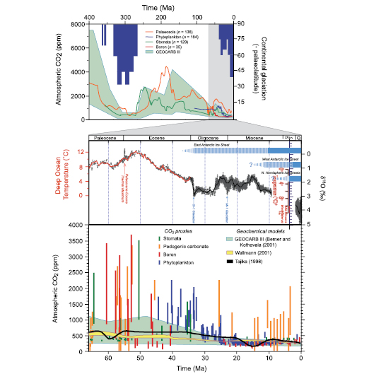
Figure 6.1. (Top) Atmospheric CO2 and continental glaciation 400 Ma to present. Vertical blue bars mark the timing and palaeolatitudinal extent of ice sheets (after Crowley, 1998 [NPR, PoC, MoS] ). Plotted CO2 records represent five-point running averages from each of the four major proxies (see ( Royer, 2006 ) for details of compilation). Also plotted are the plausible ranges of CO2 from the geochemical carbon cycle model GEOCARB III ( Berner and Kothavala, 2001 [MoS] ). All data have been adjusted to the Gradstein et al. 2004 [NPR] ) time scale. (Middle) Global compilation of deep-sea benthic foraminifera 18Oisotope records from 40 Deep Sea Drilling Program and Ocean Drilling Program sites ( Zachos et al., 2001 [JoC, SRC] ) updated with high-resolution records for the Eocene through Miocene interval ( Billups et al., 2002 [JoC, SRC] ; Bohaty and Zachos, 2003 [SRC] ; Lear et al., 2004 [JoC] ). Most data were derived from analyses of two common and long-lived benthic taxa, Cibicidoides and Nuttallides. To correct for genus-specific isotope vital effects, the 18Ovalues were adjusted by +0.64 and +0.4 ( Shackleton et al., 1984 [NPR] ), respectively. The ages are relative to the geomagnetic polarity time scale of Berggren et al. 1995 [NPR] ). The raw data were smoothed using a five-point running mean, and curve-fitted with a locally weighted mean. The 18Otemperature values assume an ice-free ocean (–1.0‰ Standard Mean Ocean Water), and thus only apply to the time preceding large-scale antarctic glaciation (~35 Ma). After the early Oligocene much of the variability (~70%) in the 18Orecord reflects changes in antarctic and Northern Hemisphere ice volume, which is represented by light blue horizontal bars (e.g., Hambrey et al., 1991 [NPR] ; Wise et al., 1991 [NPR] ;( Ehrmann and Mackensen, 1992 ) ). Where the bars are dashed, they represent periods of ephemeral ice or ice sheets smaller than present, while the solid bars represent ice sheets of modern or greater size. The evolution and stability of the West Antarctic Ice Sheet (e.g., ( Lemasurier and Rocchi, 2005 ) ) remains an important area of uncertainty that could affect estimates of future sea level rise. (Bottom) Detailed record of CO2 for the last 65 Myr. Individual records of CO2 and associated errors are colour-coded by proxy method; when possible, records are based on replicate samples (see ( Royer, 2006 ) for details and data references). Dating errors are typically less than ±1 Myr. The range of error for each CO2 proxy varies considerably, with estimates based on soil nodules yielding the greatest uncertainty. Also plotted are the plausible ranges of CO2 from three geochemical carbon cycle models.
6.3.2 What Does the Record of the Mid-Pliocene Show?
The Mid-Pliocene (about 3.3 to 3.0 Ma) is the most recent time in Earth’s history when mean global temperatures were substantially warmer for a sustained period (estimated by GCMs to be about 2°C to 3°C above pre-industrial temperatures; Chandler et al., 1994 [JoC, SRC] ; Sloan et al., 1996 [PoC, JoC, MoS] ; Haywood et al., 2000 [JoC] ; Jiang et al., 2005 [JoC, MoS] ), providing an accessible example of a world that is similar in many respects to what models estimate could be the Earth of the late 21st century. The Pliocene is also recent enough that the continents and ocean basins had nearly reached their present geographic configuration. Taken together, the average of the warmest times during the middle Pliocene presents a view of the equilibrium state of a globally warmer world, in which atmospheric CO2 concentrations (estimated to be between 360 to 400 ppm) were likely higher than pre-industrial values ( Raymo and Rau, 1992 [JoC] ; Raymo et al., 1996 [JoC] ), and in which geologic evidence and isotopes agree that sea level was at least 15 to 25 m above modern levels ( (Dowsett and Cronin, 1990; ) Shackleton et al., 1995 [NPR] ), with correspondingly reduced ice sheets and lower continental aridity ( Guo et al., 2004 [JoC] ).
Both terrestrial and marine palaeoclimate proxies ( Thompson, 1991 [JoC] ; Dowsett et al., 1996 [JoC] ; Thompson and Fleming, 1996 [JoC, MoS] ) show that high latitudes were significantly warmer, but that tropical SSTs and surface air temperatures were little different from the present. The result was a substantial decrease in the lower-tropospheric latitudinal temperature gradient. For example, atmospheric GCM simulations driven by reconstructed SSTs from the Pliocene Research Interpretations and Synoptic Mapping Group ( Dowsett et al., 1996 [JoC] ; Dowsett et al., 2005 [JoC, SRC] ) produced winter surface air temperature warming of 10°C to 20°C at high northern latitudes with 5°C to 10°C increases over the northern North Atlantic (~60°N), whereas there was essentially no tropical surface air temperature change (or even slight cooling) ( Chandler et al., 1994 [JoC, SRC] ; Sloan et al., 1996 [PoC, JoC, MoS] ; Haywood et al., 2000 [JoC] , Jiang et al., 2005 [JoC, MoS] ). In contrast, a coupled atmosphere-ocean experiment with an atmospheric CO2 concentration of 400 ppm produced warming relative to pre-industrial times of 3°C to 5°C in the northern North Atlantic, and 1°C to 3°C in the tropics ( (Haywood et al., 2005 ) ), generally similar to the response to higher CO2 discussed in Chapter 10 .
The estimated lack of tropical warming is a result of basing tropical SST reconstructions on marine microfaunal evidence. As in the case of the Last Glacial Maximum (see Section 6.4 ), it is uncertain whether tropical sensitivity is really as small as such reconstructions suggest. ( Haywood et al. 2005 ) ) found that alkenone estimates of tropical and subtropical temperatures do indicate warming in these regions, in better agreement with GCM simulations from increased CO2 forcing (see Chapter 10 ). As in the study noted above, climate models cannot produce a response to increased CO2 with large high-latitude warming, and yet minimal tropical temperature change, without strong increases in ocean heat transport ( Rind and Chandler, 1991 [JoC, SRC] ).
The substantial high-latitude response is shown by both marine and terrestrial palaeodata, and it may indicate that high latitudes are more sensitive to increased CO2 than model simulations suggest for the 21st century. Alternatively, it may be the result of increased ocean heat transports due to either an enhanced thermohaline circulation ( Raymo et al., 1989 [JoC] ; Rind and Chandler, 1991 [JoC, SRC] ) or increased flow of surface ocean currents due to greater wind stresses ( Ravelo et al., 1997 [JoC] ; Haywood et al., 2000 [JoC] ), or associated with the reduced extent of land and sea ice ( Jansen et al., 2000 [PoC, JoC, SRC] ;( Knies et al., 2002; ) ( Haywood et al., 2005 ) ). Currently available proxy data are equivocal concerning a possible increase in the intensity of the meridional overturning cell for either transient or equilibrium climate states during the Pliocene, although an increase would contrast with the North Atlantic transient deep-water production decreases that are found in most coupled model simulations for the 21st century (see Chapter 10 ). The transient response is likely to be different from an equilibrium response as climate warms. Data are just beginning to emerge that describe the deep ocean state during the Pliocene ( Cronin et al., 2005 [JoC] ). Understanding the climate distribution and forcing for the Pliocene period may help improve predictions of the likely response to increased CO2 in the future, including the ultimate role of the ocean circulation in a globally warmer world.
6.3.3 What Does the Record of the Palaeocene-Eocene Thermal Maximum Show?
Approximately 55 Ma, an abrupt warming (in this case of the order of 1 to 10 kyr) by several degrees celsius is indicated by changes in 18Oisotope and Mg/Ca records ( Kennett and Stott, 1991 [JoC, SRC] ; Zachos et al., 2003 [JoC, SRC] ; Tripati and Elderfield, 2004 [NPR] ). The warming and associated environmental impact was felt at all latitudes, and in both the surface and deep ocean. The warmth lasted approximately 100 kyr. Evidence for shifts in global precipitation patterns is present in a variety of fossil records including vegetation ( Wing et al., 2005 [JoC] ). The climate anomaly, along with an accompanying carbon isotope excursion, occurred at the boundary between the Palaeocene and Eocene epochs, and is therefore often referred to as the Palaeocene-Eocene Thermal Maximum (PETM). The thermal maximum clearly stands out in high-resolution records of that time( Figure 6.2 ). At the same time, 13Cisotopes in marine and continental records show that a large mass of carbon with low 13Cconcentration must have been released into the atmosphere and ocean. The mass of carbon was sufficiently large to lower the pH of the ocean and drive widespread dissolution of seafloor carbonates ( Zachos et al., 2005 [JoC, SRC] ). Possible sources for this carbon could have been methane (CH4)from decomposition of clathrates on the sea floor, CO2 from volcanic activity, or oxidation of sediments rich in organic matter ( Dickens et al., 1997 [MoS] ; Kurtz et al., 2003 [JoC] ; Svensen et al., 2004 [JoC] ). The PETM, which altered ecosystems worldwide ( Koch et al., 1992 [JoC, SRC] ; Bowen et al., 2002 [JoC] ; Bralower, 2002 [JoC] ;( Crouch et al., 2003; ) Thomas, 2003 [NPR] ; Bowen et al., 2004 [JoC] ;( Harrington et al., 2004 ) ), is being intensively studied as it has some similarity with the ongoing rapid release of carbon into the atmosphere by humans. The estimated magnitude of carbon release for this time period is of the order of 1 to 2 × 10¹⁸ g of carbon ( Dickens et al., 1997 [MoS] ), a similar magnitude to that associated with greenhouse gas releases during the coming century. Moreover, the period of recovery through natural carbon sequestration processes, about 100 kyr, is similar to that forecast for the future. As in the case of the Pliocene, the high-latitude warming during this event was substantial (~20°C; Moran et al., 2006 [JoC] ) and considerably higher than produced by GCM simulations for the event ( Sluijs et al., 2006 [JoC] ) or in general for increased greenhouse gas experiments( Chapter 10 ). Although there is still too much uncertainty in the data to derive a quantitative estimate of climate sensitivity from the PETM, the event is a striking example of massive carbon release and related extreme climatic warming.
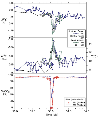
Figure 6.2. The Palaeocene-Eocene Thermal Maximum as recorded in benthic (bottom dwelling) foraminifer (Nuttallides truempyi) isotopic records from sites in the Antarctic, south Atlantic and Pacific (see Zachos et al., 2003 [JoC, SRC] for details). The rapid decrease in carbon isotope ratios in the top panel is indicative of a large increase in atmospheric greenhouse gases CO2 and CH4 that was coincident with an approximately 5°C global warming (centre panel). Using the carbon isotope records, numerical models show that CH4 released by the rapid decomposition of marine hydrates might have been a major component (~2,000 GtC) of the carbon flux ( Dickens and Owen, 1996 [JoC] ). Testing of this and other models requires an independent constraint on the carbon fluxes. In theory, much of the additional greenhouse carbon would have been absorbed by the ocean, thereby lowering seawater pH and causing widespread dissolution of seafloor carbonates. Such a response is evident in the lower panel, which shows a transient reduction in the carbonate (CaCO3)content of sediments in two cores from the south Atlantic ( Zachos et al., 2004 [NPR, SRC] , 2005 ). The observed patterns indicate that the ocean’s carbonate saturation horizon rapidly shoaled more than 2 km, and then gradually recovered as buffering processes slowly restored the chemical balance of the ocean. Initially, most of the carbonate dissolution is of sediment deposited prior to the event, a process that offsets the apparent timing of the dissolution horizon relative to the base of the benthic foraminifer carbon isotope excursion. Model simulations show that the recovery of the carbonate saturation horizon should precede the recovery in the carbon isotopes by as much as 100 kyr ( Dickens and Owen, 1996 [JoC] ), another feature that is evident in the sediment records.
6.4 Glacial-Interglacial Variability and Dynamics
6.4.1 Climate Forcings and Responses Over Glacial-Interglacial Cycles
Palaeoclimatic records document a sequence of glacial-interglacial cycles covering the last 740 kyr in ice cores (EPICA community members, 2004 ), and several million years in deep oceanic sediments ( Lisiecki and Raymo, 2005 [JoC] ) and loess ( Ding et al., 2002 [JoC] ). The last 430 kyr, which are the best documented, are characterised by 100-kyr glacial-interglacial cycles of very large amplitude, as well as large climate changes corresponding to other orbital periods ( Hays et al., 1976 [JoC] ; Box 6.1 ), and at millennial time scales ( (McManus et al., 2002; ) NorthGRIP, 2004 ). A minor proportion (20% on average) of each glacial-interglacial cycle was spent in the warm interglacial mode, which normally lasted for 10 to 30 kyr( Figure 6.3 ). There is evidence for longer interglacial periods between 430 and 740 ka, but these were apparently colder than the typical interglacials of the latest Quaternary (EPICA community members, 2004 ). The Holocene, the latest of these interglacials, extends to the present.
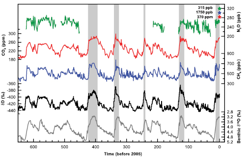
Figure 6.3. Variations of deuterium (δD; black), a proxy for local temperature, and the atmospheric concentrations of the greenhouse gases CO2 (red), CH4 (blue), and nitrous oxide (N2O; green) derived from air trapped within ice cores from Antarctica and from recent atmospheric measurements ( Petit et al., 1999 [JoC] ; Indermühle et al., 2000 [JoC] ; EPICA community members, 2004; Spahni et al., 2005 [JoC, SRC] ; Siegenthaler et al., 2005a [JoC] ,b). The shading indicates the last interglacial warm periods. Interglacial periods also existed prior to 450 ka, but these were apparently colder than the typical interglacials of the latest Quaternary. The length of the current interglacial is not unusual in the context of the last 650 kyr. The stack of 57 globally distributed benthic δ18Omarine records (dark grey), a proxy for global ice volume fluctuations ( Lisiecki and Raymo, 2005 [JoC] ), is displayed for comparison with the ice core data. Downward trends in the benthic δ18Ocurve reflect increasing ice volumes on land. Note that the shaded vertical bars are based on the ice core age model (EPICA community members, 2004 ), and that the marine record is plotted on its original time scale based on tuning to the orbital parameters ( Lisiecki and Raymo, 2005 [JoC] ). The stars and labels indicate atmospheric concentrations at year 2000 .
Box 6.1: Orbital Forcing
It is well known from astronomical calculations ( Berger, 1978 [ARC] ) that periodic changes in parameters of the orbit of the Earth around the Sun modify the seasonal and latitudinal distribution of incoming solar radiation at the top of the atmosphere (hereafter called ‘insolation’). Past and future changes in insolation can be calculated over several millions of years with a high degree of confidence ( Berger and Loutre, 1991 [JoC, SRC] ;( Laskar et al., 2004 ) ). This box focuses on the time period from the past 800 kyr to the next 200 kyr.
Over this time interval, the obliquity (tilt) of the Earth axis varies between 22.05° and 24.50° with a strong quasi-periodicity around 41 kyr. Changes in obliquity have an impact on seasonal contrasts. This parameter also modulates annual mean insolation changes with opposite effects in low vs. high latitudes (and therefore no effect on global average insolation). Local annual mean insolation changes remain below 6 Wm–2.
The eccentricity of the Earth’s orbit around the Sun has longer quasi-periodicities at 400 and around 100 kyr, and varies between values of about 0.002 and 0.050 during the time period from 800 ka to 200 kyr in the future. Changes in eccentricity alone modulate the Sun-Earth distance and have limited impacts on global and annual mean insolation. However, changes in eccentricity affect the intra-annual changes in the Sun-Earth distance and thereby modulate significantly the seasonal and latitudinal effects induced by obliquity and climatic precession.
Associated with the general precession of the equinoxes and the longitude of perihelion, periodic shifts in the position of solstices and equinoxes on the orbit relative to the perihelion occur, and these modulate the seasonal cycle of insolation with periodicities of about 19 and about 23 kyr. As a result, changes in the position of the seasons on the orbit strongly modulate the latitudinal and seasonal distribution of insolation. When averaged over a season, insolation changes can reach 60 Wm–2 (Box 6.1, Figure 1). During periods of low eccentricity, such as about 400 ka and during the next 100 kyr, seasonal insolation changes induced by precession are less strong than during periods of larger eccentricity (Box 6.1, Figure 1). High-frequency variations of orbital variations appear to be associated with very small insolation changes ( Bertrand et al., 2002a [NPR, JoC, SRC] ).
The Milankovitch theory proposes that ice ages are triggered by minima in summer insolation near 65°N, enabling winter snowfall to persist all year and therefore accumulate to build NH glacial ice sheets. For example, the onset of the last ice age, about 116 ± 1 ka ( Stirling et al., 1998 [ARC] ), corresponds to a 65°N mid-June insolation about 40 Wm–2 lower than today (Box 6.1, Figure 1).
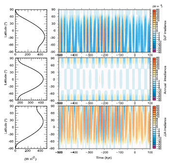
Box 6.1 ,Figure 1. (Left) December to February (top), annual mean (middle) and June to August (bottom) latitudinal distribution of present-day (year 1950 ) incoming mean solar radiation (Wm–2). (Right) Deviations with respect to the present of December to February (top), annual mean (middle) and June to August (bottom) latitudinal distribution of incoming mean solar radiation (Wm–2)from the past 500 kyr to the future 100 kyr ( Berger and Loutre, 1991 [JoC, SRC] ; Loutre et al., 2004 [SRC] ).
Studies of the link between orbital parameters and past climate changes include spectral analysis of palaeoclimatic records and the identification of orbital periodicities; precise dating of specific climatic transitions; and modelling of the climate response to orbital forcing, which highlights the role of climatic and biogeochemical feedbacks. Sections 6.4 and 6.5 describe some aspects of the state-of-the-art understanding of the relationships between orbital forcing, climate feedbacks and past climate changes.
The ice core record indicates that greenhouse gases co-varied with antarctic temperature over glacial-interglacial cycles, suggesting a close link between natural atmospheric greenhouse gas variations and temperature( Box 6.2 ). Variations in CO2 over the last 420 kyr broadly followed antarctic temperature, typically by several centuries to a millennium ( Mudelsee, 2001 [JoC] ). The sequence of climatic forcings and responses during deglaciations (transitions from full glacial conditions to warm interglacials) are well documented. High-resolution ice core records of temperature proxies and CO2 during deglaciation indicates that antarctic temperature starts to rise several hundred years before CO2 ( Monnin et al., 2001 [JoC, SRC] ; Caillon et al., 2003 [JoC] ). During the last deglaciation, and likely also the three previous ones, the onset of warming at both high southern and northern latitudes preceded by several thousand years the first signals of significant sea level increase resulting from the melting of the northern ice sheets linked with the rapid warming at high northern latitudes ( Petit et al., 1999 [JoC] ; Shackleton, 2000 [JoC] ; Pépin et al., 2001 [JoC, MoS, SRC] ). Current data are not accurate enough to identify whether warming started earlier in the Southern Hemisphere (SH) or Northern Hemisphere (NH), but a major deglacial feature is the difference between North and South in terms of the magnitude and timing of strong reversals in the warming trend, which are not in phase between the hemispheres and are more pronounced in the NH ( Blunier and Brook, 2001 [JoC] ).
Greenhouse gas (especially CO2)feedbacks contributed greatly to the global radiative perturbation corresponding to the transitions from glacial to interglacial modes (see Section 6.4.1.2 ). The relationship between antarctic temperature and CO2 did not change significantly during the past 650 kyr, indicating a rather stable coupling between climate and the carbon cycle during the late Pleistocene ( Siegenthaler et al., 2005a [JoC] ). The rate of change in atmospheric CO2 varied considerably over time. For example, the CO2 increase from about 180 ppm at the Last Glacial Maximum to about 265 ppm in the early Holocene occurred with distinct rates over different periods ( Monnin et al., 2001 [JoC, SRC] ; Figure 6.4 ).
Box 6.2: What Caused the Low Atmospheric Carbon Dioxide Concentrations During Glacial Times?
Ice core records show that atmospheric CO2 varied in the range of 180 to 300 ppm over the glacial-interglacial cycles of the last 650 kyr( Figure 6.3 ;Petit et al., 1999 [JoC] ; Siegenthaler et al., 2005a [JoC] ). The quantitative and mechanistic explanation of these CO2 variations remains one of the major unsolved questions in climate research. Processes in the atmosphere, in the ocean, in marine sediments and on land, and the dynamics of sea ice and ice sheets must be considered. A number of hypotheses for the low glacial CO2 concentrations have emerged over the past 20 years, and a rich body of literature is available ( Webb et al., 1997 [JoC] ; Broecker and Henderson, 1998 [JoC] ; Archer et al., 2000 [JoC, ARC] ; Sigman and Boyle, 2000 [JoC] ; Kohfeld et al., 2005 [JoC, ARC] ). Many processes have been identified that could potentially regulate atmospheric CO2 on glacial-interglacial time scales. However, the existing proxy data with which to test hypotheses are relatively scarce, uncertain, and their interpretation is partly conflicting.
Most explanations propose changes in oceanic processes as the cause for low glacial CO2 concentrations. The ocean is by far the largest of the relatively fast-exchanging (<1 kyr) carbon reservoirs, and terrestrial changes cannot explain the low glacial values because terrestrial storage was also low at the Last Glacial Maximum (see Section 6.4.1 ). On glacial-interglacial time scales, atmospheric CO2 is mainly governed by the interplay between ocean circulation, marine biological activity, ocean-sediment interactions, seawater carbonate chemistry and air-sea exchange. Upon dissolution in seawater, CO2 maintains an acid/base equilibrium with bicarbonate and carbonate ions that depends on the acid-titrating capacity of seawater (i.e., alkalinity). Atmospheric CO2 would be higher if the ocean lacked biological activity. CO2 is more soluble in colder than in warmer waters; therefore, changes in surface and deep ocean temperature have the potential to alter atmospheric CO2.Most hypotheses focus on the Southern Ocean, where large volume- fractions of the cold deep-water masses of the world ocean are currently formed, and large amounts of biological nutrients (phosphate and nitrate) upwelling to the surface remain unused. A strong argument for the importance of SH processes is the co-evolution of antarctic temperature and atmospheric CO2.
One family of hypotheses regarding low glacial atmospheric CO2 values invokes an increase or redistribution in the ocean alkalinity as a primary cause. Potential mechanisms are (i) the increase of calcium carbonate (CaCO3)weathering on land, (ii) a decrease of coral reef growth in the shallow ocean, or (iii) a change in the export ratio of CaCO3 and organic material to the deep ocean. These mechanisms require large changes in the deposition pattern of CaCO3 to explain the full amplitude of the glacial-interglacial CO2 difference through a mechanism called carbonate compensation ( Archer et al., 2000 [JoC, ARC] ). The available sediment data do not support a dominant role for carbonate compensation in explaining low glacial CO2 levels. Furthermore, carbonate compensation may only explain slow CO2 variation, as its time scale is multi-millennial.
Another family of hypotheses invokes changes in the sinking of marine plankton. Possible mechanisms include (iv) fertilization of phytoplankton growth in the Southern Ocean by increased deposition of iron-containing dust from the atmosphere after being carried by winds from colder, drier continental areas, and a subsequent redistribution of limiting nutrients; (v) an increase in the whole ocean nutrient content (e.g., through input of material exposed on shelves or nitrogen fixation); and (vi) an increase in the ratio between carbon and other nutrients assimilated in organic material, resulting in a higher carbon export per unit of limiting nutrient exported. As with the first family of hypotheses, this family of mechanisms also suffers from the inability to account for the full amplitude of the reconstructed CO2 variations when constrained by the available information. For example, periods of enhanced biological production and increased dustiness (iron supply) are coincident with CO2 concentration changes of 20 to 50 ppm (see Section 6.4.2 , Figure 6.7 ). Model simulations consistently suggest a limited role for iron in regulating past atmospheric CO2 concentration ( Bopp et al., 2002 [ARC] ).
Physical processes also likely contributed to the observed CO2 variations. Possible mechanisms include (vii) changes in ocean temperature (and salinity), (viii) suppression of air-sea gas exchange by sea ice, and (ix) increased stratification in the Southern Ocean. The combined changes in temperature and salinity increased the solubility of CO2,causing a depletion in atmospheric CO2 of perhaps 30 ppm. Simulations with general circulation ocean models do not fully support the gas exchange-sea ice hypothesis. One explanation (ix) conceived in the 1980 s invokes more stratification, less upwelling of carbon and nutrient-rich waters to the surface of the Southern Ocean and increased carbon storage at depth during glacial times. The stratification may have caused a depletion of nutrients and carbon at the surface, but proxy evidence for surface nutrient utilisation is controversial. Qualitatively, the slow ventilation is consistent with very saline and very cold deep waters reconstructed for the last glacial maximum ( Adkins et al., 2002 [JoC] ), as well as low glacial stable carbon isotope ratios(13C/12C) in the deep South Atlantic.
In conclusion, the explanation of glacial-interglacial CO2 variations remains a difficult attribution problem. It appears likely that a range of mechanisms have acted in concert (e.g., Köhler et al., 2005 [PoC, JoC, MoS, SRC] ). The future challenge is not only to explain the amplitude of glacial-interglacial CO2 variations, but the complex temporal evolution of atmospheric CO2 and climate consistently.
6.4.1.1 How Do Glacial-Interglacial Variations in the Greenhouse Gases Carbon Dioxide, Methane and Nitrous Oxide Compare with the Industrial Era Greenhouse Gas Increase?
The present atmospheric concentrations of CO2,CH4 and nitrous oxide (N2O) are higher than ever measured in the ice core record of the past 650 kyr (Figures 6.3 and 6.4 ). The measured concentrations of the three greenhouse gases fluctuated only slightly (within 4% for CO2 andN2Oand within 7% for CH4)over the past millennium prior to the industrial era, and also varied within a restricted range over the late Quaternary. Within the last 200 years, the late Quaternary natural range has been exceeded by at least 25% for CO2,120% for CH4 and 9% forN2O. All three records show effects of the large and increasing growth in anthropogenic emissions during the industrial era.
Variations in atmospheric CO2 dominate the radiative forcing by all three gases( Figure 6.4 ). The industrial era increase in CO2,and in the radiative forcing( Section 2.3 )by all three gases, is similar in magnitude to the increase over the transitions from glacial to interglacial periods, but started from an interglacial level and occurred one to two orders of magnitude faster ( Stocker and Monnin, 2003 [MoS, SRC] ). There is no indication in the ice core record that an increase comparable in magnitude and rate to the industrial era has occurred in the past 650 kyr. The data resolution is sufficient to exclude with very high confidence a peak similar to the anthropogenic rise for the past 50 kyr for CO2,for the past 80 kyr for CH4 and for the past 16 kyr forN2O. The ice core records show that during the industrial era, the average rate of increase in the radiative forcing from CO2,CH4 andN2Ois greater than at any time during the past 16 kyr( Figure 6.4 ). The smoothing of the atmospheric signal ( Schwander et al., 1993 [JoC] ; Spahni et al., 2003 [JoC, SRC] ) is small at Law Dome, a high-accumulation site in Antarctica, and decadal-scale rates of change can be computed from the Law Dome record spanning the past two millennia ( Etheridge et al., 1996 [JoC, ARC] ; Ferretti et al., 2005 [JoC] ; MacFarling Meure et al., 2006 [JoC] ). The average rate of increase in atmospheric CO2 was at least five times larger over the period from 1960 to 1999 than over any other 40-year period during the two millennia before the industrial era. The average rate of increase in atmospheric CH4 was at least six times larger, and that forN2Oat least two times larger over the past four decades, than at any time during the two millennia before the industrial era. Correspondingly, the recent average rate of increase in the combined radiative forcing by all three greenhouse gases was at least six times larger than at any time during the period AD 1 to AD 1800 ( Figure 6.4 d).
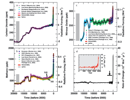
Figure 6.4. The concentrations and radiative forcing by (a) CO2,(b) CH4 and (c) nitrous oxide (N2O), and (d) the rate of change in their combined radiative forcing over the last 20 kyr reconstructed from antarctic and Greenland ice and firn data (symbols) and direct atmospheric measurements (red and magenta lines). The grey bars show the reconstructed ranges of natural variability for the past 650 kyr ( Siegenthaler et al., 2005a [JoC] ; Spahni et al., 2005 [JoC, SRC] ). Radiative forcing was computed with the simplified expressions of Chapter2 ( Myhre et al., 1998 [JoC, MoS, ARC] ). The rate of change in radiative forcing (black line) was computed from spline fits ( Enting, 1987 [JoC] ) of the concentration data (black lines in panels a to c). The width of the age distribution of the bubbles in ice varies from about 20 years for sites with a high accumulation of snow such as Law Dome, Antarctica, to about 200 years for low-accumulation sites such as Dome C, Antarctica. The Law Dome ice and firn data, covering the past two millennia, and recent instrumental data have been splined with a cut-off period of 40 years, with the resulting rate of change in radiative forcing shown by the inset in (d). The arrow shows the peak in the rate of change in radiative forcing after the anthropogenic signals of CO2,CH4 andN2Ohave been smoothed with a model describing the enclosure process of air in ice ( Spahni et al., 2003 [JoC, SRC] ) applied for conditions at the low accumulation Dome C site for the last glacial transition. The CO2 data are from Etheridge et al. 1996 [JoC, ARC] Monnin et al. 2001 [JoC, SRC] Monnin et al. 2004 [SRC] Siegenthaler et al. 2005b [JoC] ; South Pole); Siegenthaler et al. 2005a [JoC] ; Kohnen Station); and MacFarling Meure et al. 2006 [JoC] ). The CH4 data are from Stauffer et al. 1985 [JoC] Steele et al. 1992 [JoC] Blunier et al. 1993 [JoC] Dlugokencky et al. 1994 [JoC, ARC] Blunier et al. 1995 [JoC] Chappellaz et al. 1997 [JoC] Monnin et al. 2001 [JoC, SRC] Flückiger et al. 2002 [NPR, JoC] and Ferretti et al. 2005 [JoC] ). TheN2Odata are from Machida et al. 1995 [JoC] Battle et al. 1996 [JoC] Flückiger et al. 1999 [JoC] , 2002 and MacFarling Meure et al. 2006 [JoC] ). Atmospheric data are from the National Oceanic and Atmospheric Administration’s global air sampling network, representing global average concentrations (dry air mole fraction; Steele et al., 1992 [JoC] ; Dlugokencky et al., 1994 [JoC, ARC] ; Tans and Conway, 2005 [NPR, ARC] ), and from Mauna Loa, Hawaii ( Keeling and Whorf, 2005 [NPR, ARC] ). The globally averaged data are available from http://www.cmdl.noaa.gov/.
6.4.1.2 What Do the Last Glacial Maximum and the Last Deglaciation Show?
Past glacial cold periods, sometimes referred to as ‘ice ages’, provide a means for evaluating the understanding and modelling of the response of the climate system to large radiative perturbations. The most recent glacial period started about 116 ka, in response to orbital forcing( Box 6.1 ), with the growth of ice sheets and fall of sea level culminating in the Last Glacial Maximum (LGM), around 21 ka. The LGM and the subsequent deglaciation have been widely studied because the radiative forcings, boundary conditions and climate response are relatively well known.
The response of the climate system at the LGM included feedbacks in the atmosphere and on land amplifying the orbital forcing. Concentrations of well-mixed greenhouse gases at the LGM were reduced relative to pre-industrial values (Figures 6.3 and 6.4 ), amounting to a global radiative perturbation of –2.8 Wm–2 – approximately equal to, but opposite from, the radiative forcing of these gases for the year 2000 (see Section 2.3 ). Land ice covered large parts of North America and Europe at the LGM, lowering sea level and exposing new land. The radiative perturbation of the ice sheets and lowered sea level, specified as a boundary condition for some LGM simulations, has been estimated to be about –3.2 Wm–2,but with uncertainties associated with the coverage and height of LGM continental ice ( Mangerud et al., 2002 [JoC] ; Peltier, 2004 [MoS] ; Toracinta et al., 2004 [JoC, ARC] ; Masson-Delmotte et al., 2006 [JoC, MoS, SRC] ) and the parametrization of ice albedo in climate models ( Taylor et al., 2000 [NPR, MoS, ARC] ). The distribution of vegetation was altered, with tundra expanded over the northern continents and tropical rain forest reduced ( (Prentice et al., 2000 ) ), and atmospheric aerosols (primarily dust) were increased ( (Kohfeld and Harrison, 2001 ) ), partly as a consequence of reduced vegetation cover ( Mahowald et al., 1999 [JoC, MoS] ). Vegetation and atmospheric aerosols are treated as specified conditions in some LGM simulations, each contributing about –1 Wm–2 of radiative perturbation, but with very low scientific understanding of their radiative influence at the LGM ( Claquin et al., 2003 [JoC, MoS] ; Crucifix and Hewitt, 2005 [JoC] ). Changes in biogeochemical cycles thus played an important role and contributed, through changes in greenhouse gas concentration, dust loading and vegetation cover, more than half of the known radiative perturbation during the LGM. Overall, the radiative perturbation for the changed greenhouse gas and aerosol concentrations and land surface was approximately –8 Wm–2 for the LGM, although with significant uncertainty in the estimates for the contributions of aerosol and land surface changes( Figure 6.5 ).
Understanding of the magnitude of tropical cooling over land at the LGM has improved since the TAR with more records, as well as better dating and interpretation of the climate signal associated with snow line elevation and vegetation change. Reconstructions of terrestrial climate show strong spatial differentiation, regionally and with elevation. Pollen records with their extensive spatial coverage indicate that tropical lowlands were on average 2°C to 3°C cooler than present, with strong cooling (5°C–6°C) in Central America and northern South America and weak cooling (<2°C) in the western Pacific Rim ( Farrera et al., 1999 [JoC] ). Tropical highland cooling estimates derived from snow-line and pollen-based inferences show similar spatial variations in cooling although involving substantial uncertainties from dating and mapping, multiple climatic causes of treeline and snow line changes during glacial periods ( Porter, 2001 [JoC] ; Kageyama et al., 2004 [NPR, JoC, SRC] ), and temporal asynchroneity between different regions of the tropics ( Smith et al., 2005 [JoC] ). These new studies give a much richer regional picture of tropical land cooling, and stress the need to use more than a few widely scattered proxy records as a measure of low-latitude climate sensitivity ( (Harrison, 2005 ) ).
The Climate: Long-range Investigation, Mapping, and Prediction (CLIMAP) reconstruction of ocean surface temperatures produced in the early 1980 s indicated about 3°C cooling in the tropical Atlantic, and little or no cooling in the tropical Pacific. More pronounced tropical cooling for the LGM tropical oceans has since been proposed, including 4°C to 5°C based on coral skeleton records from off Barbados ( Guilderson et al., 1994 [JoC] ) and up to 6°C in the cold tongue off western South America based on foraminiferal assemblages ( Mix et al., 1999 [JoC, MoS] ). New data syntheses from multiple proxy types using carefully defined chronostratigraphies and new calibration data sets are now available from the Glacial Ocean Mapping (GLAMAP) and Multiproxy Approach for the Reconstruction of the Glacial Ocean surface (MARGO) projects, although with caveats including selective species dissolution, dating precision, non-analogue situations, and environmental preferences of the organisms ( Sarnthein et al., 2003b [JoC] ; Kucera et al., 2005 [JoC] ; and references therein). These recent reconstructions confirm moderate cooling, generally 0°C to 3.5°C, of tropical SST at the LGM, although with significant regional variation, as well as greater cooling in eastern boundary currents and equatorial upwelling regions. Estimates of cooling show notable differences among the different proxies. Faunal-based proxies argue for an intensification of the eastern equatorial Pacific cold tongue in contrast to Mg/Ca-based SST estimates that suggest a relaxation of SST gradients within the cold tongue ( Mix et al., 1999 [JoC, MoS] ; Koutavas et al., 2002 [JoC] ; Rosenthal and Broccoli, 2004 [JoC, ARC] ). Using a Bayesian approach to combine different proxies, Ballantyne et al. 2005 [JoC] ) estimated a LGM cooling of tropical SSTs of 2.7°C ± 0.5°C (1 standard deviation).
These ocean proxy synthesis projects also indicate a colder glacial winter North Atlantic with more extensive sea ice than present, whereas summer sea ice only covered the glacial Arctic Ocean and Fram Strait with the northern North Atlantic and Nordic Seas largely ice free and more meridional ocean surface circulation in the eastern parts of the Nordic Seas ( Sarnthein et al., 2003a [NPR, JoC, MoS] ; Meland et al., 2005 [PoC, JoC, MoS, SRC] ;( de Vernal et al., 2006 ) ). Sea ice around Antarctica at the LGM also responded with a large expansion of winter sea ice and substantial seasonal variation ( Gersonde et al., 2005 [JoC] ). Over mid- and high-latitude northern continents, strong reductions in temperatures produced southward displacement and major reductions in forest area ( Bigelow et al., 2003 [JoC] ), expansion of permafrost limits over northwest Europe ( Renssen and Vandenberghe, 2003 [JoC, ARC] ), fragmentation of temperate forests ( (Prentice et al., 2000; ) ( Williams et al., 2000 ) ) and predominance of steppe-tundra in Western Europe ( (Peyron et al., 2005 ) ). Temperature reconstructions from polar ice cores indicate strong cooling at high latitudes of about 9°C in Antarctica ( Stenni et al., 2001 [JoC] ) and about 21°C in Greenland ( Dahl-Jensen et al., 1998 [JoC] ).
The strength and depth extent of the LGM Atlantic overturning circulation have been examined through the application of a variety of new marine proxy indicators ( Rutberg et al., 2000 [JoC] ; Duplessy et al., 2002 [JoC, SRC] ; Marchitto et al., 2002 [JoC] ; McManus et al., 2004 [JoC] ). These tracers indicate that the boundary between North Atlantic Deep Water (NADW) and Antarctic Bottom Water was much shallower during the LGM, with a reinforced pycnocline between intermediate and particularly cold and salty deep water ( Adkins et al., 2002 [JoC] ). Most of the deglaciation occurred over the period about 17 to 10 ka, the same period of maximum deglacial atmospheric CO2 increase( Figure 6.4 ). It is thus very likely that the global warming of 4°C to 7°C since the LGM occurred at an average rate about 10 times slower than the warming of the 20th century.
In summary, significant progress has been made in the understanding of regional changes at the LGM with the development of new proxies, many new records, improved understanding of the relationship of the various proxies to climate variables and syntheses of proxy records into reconstructions with stricter dating and common calibrations.
6.4.1.3 How Realistic Are Results from Climate Model Simulations of the Last Glacial Maximum?
Model intercomparisons from the first phase of the Paleoclimate Modelling Intercomparison Project (PMIP-1), using atmospheric models (either with prescribed SST or with simple slab ocean models), were featured in the TAR. There are now six simulations of the LGM from the second phase (PMIP-2) using Atmosphere-Ocean General Circulation Models (AOGCMs) and EMICs, although only a few regional comparisons were completed in time for this assessment. The radiative perturbation for the PMIP-2 LGM simulations available for this assessment, which do not yet include the effects of vegetation or aerosol changes, is –4 to –7 Wm–2.These simulations allow an assessment of the response of a subset of the models presented in Chapters 8 and 10 to very different conditions at the LGM.
The PMIP-2 multi-model LGM SST change shows a modest cooling in the tropics, and greatest cooling at mid- to high latitudes in association with increases in sea ice and changes in ocean circulation( Figure 6.5 ). The PMIP-2 modelled strengthening of the SST meridional gradient in the LGM North Atlantic, as well as cooling and expanded sea ice, agrees with proxy indicators ( Kageyama et al., 2006 [JoC, MoS, SRC] ). Polar amplification of global cooling, as recorded in ice cores, is reproduced for Antarctica( Figure 6.5 ), but the strong LGM cooling over Greenland is underestimated, although with caveats about the heights of these ice caps in the PMIP-2 simulations ( Masson-Delmotte et al., 2006 [JoC, MoS, SRC] ).
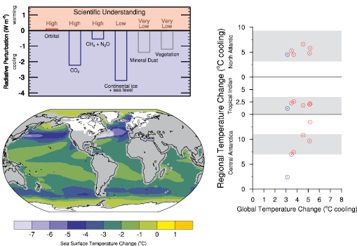
Figure 6.5. The Last Glacial Maximum climate (approximately 21 ka) relative to the pre-industrial ( 1750 ) climate. (Top left) Global annual mean radiative influences (Wm–2)of LGM climate change agents, generally feedbacks in glacial-interglacial cycles, but also specified in most Atmosphere-Ocean General Circulation Model (AOGCM) simulations for the LGM. The heights of the rectangular bars denote best estimate values guided by published values of the climate change agents and conversion to radiative perturbations using simplified expressions for the greenhouse gas concentrations and model calculations for the ice sheets, vegetation and mineral dust. References are included in the text. A judgment of each estimate’s reliability is given as a level of scientific understanding based on uncertainties in the climate change agents and physical understanding of their radiative effects. Paleoclimate Modelling Intercomparison Project 2 (PMIP-2) simulations shown in bottom left and right panels do not include the radiative influences of LGM changes in mineral dust or vegetation. (Bottom left) Multi-model average SST change for LGM PMIP-2 simulations by five AOGCMs (Community Climate System Model (CCSM), Flexible Global Ocean-Atmosphere-Land System (FGOALS), Hadley Centre Coupled Model (HadCM), Institut Pierre Simon Laplace Climate System Model (IPSL-CM), Model for Interdisciplinary Research on Climate (MIROC)). Ice extent over continents is shown in white. (Right) LGM regional cooling compared to LGM global cooling as simulated in PMIP-2, with AOGCM results shown as red circles and EMIC (ECBilt-CLIO) results shown as blue circles. Regional averages are defined as: Antarctica, annual for inland ice cores; tropical Indian Ocean, annual for 15°S to 15°N, 50°E to 100°E; and North Atlantic Ocean, July to September for 42°N to 57°N, 35°W to 20°E. Grey shading indicates the range of observed proxy estimates of regional cooling: Antarctica ( Stenni et al., 2001 [JoC] ; Masson-Delmotte et al., 2006 [JoC, MoS, SRC] ), tropical Indian Ocean ( Rosell-Mele et al., 2004 [JoC, MoS] ; Barrows and Juggins, 2005 [JoC] ), and North Atlantic Ocean ( Rosell-Mele et al., 2004 [JoC, MoS] ; Kucera et al., 2005 [JoC] ;( de Vernal et al., 2006; ) Kageyama et al., 2006 [JoC, MoS, SRC] ).
The PMIP-2 AOGCMs give a range of tropical ocean
cooling between 15°S to 15°N of 1.7°C to 2.4°C. Sensitivity simulations with models indicate that this tropical cooling can be explained by the reduced glacial greenhouse gas concentrations, which had direct effects on the tropical radiative forcing ( Shin et al., 2003 [JoC, MoS] ; Otto-Bliesner et al., 2006b [JoC, SRC] ) and indirect effects through LGM cooling by positive sea ice-albedo feedback in the Southern Ocean contributing to enhanced ocean ventilation of the tropical thermocline and the intermediate waters ( Liu et al., 2002 [JoC] ). Regional variations in simulated tropical cooling are much smaller than indicated by MARGO data, partly related to models at current resolutions being unable to simulate the intensity of coastal upwelling and eastern boundary currents. Simulated cooling in the Indian Ocean( Figure 6.5 ), a region with important present-day teleconnections to Africa and the North Atlantic, compares favourably to proxy estimates from alkenones ( Rosell-Mele et al., 2004 [JoC, MoS] ) and foraminifera assemblages ( Barrows and Juggins, 2005 [JoC] ).
Considering changes in vegetation appears to improve the realism of simulations of the LGM, and points to important climate-vegetation feedbacks ( Wyputta and McAvaney, 2001 [JoC, MoS, ARC] ; Crucifix and Hewitt, 2005 [JoC] ). For example, extension of the tundra in Asia during the LGM contributes to the local surface cooling, while the tropics warm where savannah replaces tropical forest ( Wyputta and McAvaney, 2001 [JoC, MoS, ARC] ). Feedbacks between climate and vegetation occur locally, with a decrease in the tree fraction in central Africa reducing precipitation, and remotely with cooling in Siberia (tundra replacing trees) altering (diminishing) the Asian summer monsoon. The physiological effect of CO2 concentration on vegetation needs to be included to properly represent changes in global forest ( Harrison and Prentice, 2003 [MoS] ), as well as to widen the climatic range where grasses and shrubs dominate. The biome distribution simulated with dynamic global vegetation models reproduces the broad features observed in palaeodata (e.g., Harrison and Prentice, 2003 [MoS] ).
In summary, the PMIP-2 LGM simulations confirm that current AOGCMs are able to simulate the broad-scale spatial patterns of regional climate change recorded by palaeodata in response to the radiative forcing and continental ice sheets of the LGM, and thus indicate that they adequately represent the primary feedbacks that determine the climate sensitivity of this past climate state to these changes. The PMIP-2 AOGCM simulations using glacial-interglacial changes in greenhouse gas forcing and ice sheet conditions give a radiative perturbation in reference to pre-industrial conditions of –4.6 to –7.2 Wm–2 and mean global temperature change of –3.3°C to –5.1°C, similar to the range reported in the TAR for PMIP-1 ( IPCC, 2001 [NPR] ). The climate sensitivity inferred from the PMIP-2 LGM simulations is 2.3°C to 3.7°C for a doubling of atmospheric CO2 (see Section 9.6.3.2 ). When the radiative perturbations of dust content and vegetation changes are estimated, climate models yield an additional cooling of 1°C to 2°C ( Crucifix and Hewitt, 2005 [JoC] ; Schneider et al., 2006 [NotFound] ), although scientific understanding of these effects is very low.
6.4.1.4 How Realistic Are Simulations of Terrestrial Carbon Storage at the Last Glacial Maximum?
There is evidence that terrestrial carbon storage was reduced during the LGM compared to today. Mass balance calculations based on 13Cmeasurements on shells of benthic foraminifera yield a reduction in the terrestrial biosphere carbon inventory (soil and living vegetation) of about 300 to 700 GtC ( Shackleton, 1977 [NPR] ; Bird et al., 1994 [JoC] ) compared to the pre-industrial inventory of about 3,000 GtC. Estimates of terrestrial carbon storage based on ecosystem reconstructions suggest an even larger difference (e.g., Crowley, 1995 [PoC, JoC] ). Simulations with carbon cycle models yield a reduction in global terrestrial carbon stocks of 600 to 1,000 GtC at the LGM compared to pre-industrial time ( Francois et al., 1998 [JoC, MoS] ; Beerling, 1999 [MoS] ;( Francois et al., 1999; ) Kaplan et al., 2002 [JoC, MoS] ; Liu et al., 2002 [JoC] ; Kaplan et al., 2003 [NPR, JoC, MoS] ; Joos et al., 2004 [PoC, JoC, MoS, SRC] ). The majority of this simulated difference is due to reduced simulated growth resulting from lower atmospheric CO2.A major regulating role for CO2 is consistent with the model-data analysis of ( Bond et al. 2003 ) ), who suggested that low atmospheric CO2 could have been a significant factor in the reduction of trees during glacial times, because of their slower regrowth after disturbances such as fire. In summary, results of terrestrial models, also used to project future CO2 concentrations, are broadly compatible with the range of reconstructed differences in glacial-interglacial carbon storage on land.
It has been suggested that Stage 11 was an extraordinarily long interglacial period because of its low orbital eccentricity, which reduces the effect of climatic precession on insolation( Box 6.1 )(Berger and Loutre, 2003 [NPR, MoS, SRC] ). In addition, the EPICA Dome C and the recently revisited Vostok records show CO2 concentrations similar to pre-industrial Holocene values throughout Stage 11 ( Raynaud et al., 2005 [JoC, SRC] ). Thus, both the orbital forcing and the CO2 feedback were providing favourable conditions for an unusually long interglacial. Moreover, the length of Stage 11 has been simulated by conceptual models of the Quaternary climate, based on threshold mechanisms ( Paillard, 1998 [JoC, MoS] ). For Stage 11, these conceptual models show that the deglaciation was triggered by the insolation maximum at about 427 ka, but that the next insolation minimum was not sufficiently low to start another glaciation. The interglacial thus lasts an additional precessional cycle, yielding a total duration of 28 kyr.
6.4.1.5 How Long Did the Previous Interglacials Last?
The four interglacials of the last 450 kyr preceding the Holocene (Marine Isotope Stages 5, 7, 9 and 11) were all different in multiple aspects, including duration( Figure 6.3 ). The shortest (Stage 7) lasted a few thousand years, and the longest (Stage 11; ~420 to 395 ka) lasted almost 30 kyr. Evidence for an unusually long Stage 11 has been recently reinforced by new ice core and marine sediment data. The European Programme for Ice Coring in Antarctica (EPICA) Dome C antarctic ice core record suggests that antarctic temperature remained approximately as warm as the Holocene for 28 kyr (EPICA community members, 2004 ). A new stack of 57 globally distributed benthic δ18Orecords presents age estimates at Stage 11 nearly identical to those provided by the EPICA results ( Lisiecki and Raymo, 2005 [JoC] ).
6.4.1.6 How Much Did the Earth Warm During the Previous Interglacial?
Globally, there was less glacial ice on Earth during the Last Interglacial, also referred to as “Last Interglaciation” (LIG, 130 ± 1 to 116 ± 1 ka; Stirling et al., 1998 [ARC] ) than now. This suggests significant reduction in the size of the Greenland and possibly Antarctic Ice Sheets (see Section 6.4.3 ). The climate of the LIG has been inferred to be warmer than present ( (Kukla et al., 2002 ) ), although the evidence is regional and not necessarily synchronous globally, consistent with understanding of the primary forcing. For the first half of this interglacial (~130–123 ka), orbital forcing( Box 6.1 )produced a large increase in NH summer insolation. Proxy data indicate warmer-than-present coastal waters in parts of the Pacific, Atlantic, and Indian Oceans as well as in the Mediterranean Sea, greatly reduced sea ice in the coastal waters around Alaska, extension of boreal forest into areas now occupied by tundra in interior Alaska and Siberia and a generally warmer Arctic ( (Brigham-Grette and Hopkins, 1995; ) ( Lozhkin and Anderson, 1995; ) Muhs et al., 2001 [JoC, SRC] , CAPE Last Interglacial Project Members, 2006 ). Ice core data indicate a large response over Greenland and Antarctica with early LIG temperatures 3°C to 5°C warmer than present ( Watanabe et al., 2003 [JoC] ; NGRIP, 2004 [JoC] ; Landais et al., 2006 [JoC] ). Palaeofauna evidence from New Zealand indicates LIG warmth during the late LIG consistent with the latitudinal dependence of orbital forcing ( (Marra, 2003 ) ).
There are AOGCM simulations available for the LIG, but no standardised intercomparison simulations have been performed. When forced with orbital forcing of 130 to 125 ka( Box 6.1 ), with over 10% more summer insolation in the NH than today, AOGCMs produce a summer arctic warming of up to 5°C, with greatest warming over Eurasia and in the Baffin Island/northern Greenland region( Figure 6.6 )(Montoya et al., 2000 [PoC, JoC, MoS] ; Kaspar et al., 2005 [JoC, MoS, ARC] ; Otto-Bliesner et al., 2006a [PoC, JoC, MoS, SRC] ). Simulations generally match proxy reconstructions of the maximum arctic summer warmth ( Kaspar and Cubasch, 2006 [NPR, ARC] ; CAPE Last Interglacial Project Members, 2006 ) although may still underestimate warmth in Siberia because vegetation feedbacks are not included in current simulations. Simulated LIG annual average global temperature is not notably higher than present, consistent with the orbital forcing.
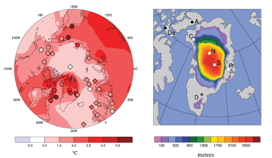
Figure 6.6. Summer surface air temperature change over the Arctic (left) and annual minimum ice thickness and extent for Greenland and western arctic glaciers (right) for the LIG from a multi-model and a multi-proxy synthesis. The multi-model summer warming simulated by the National Center for Atmospheric Research (NCAR) Community Climate System Model (CCSM), 130 ka minus present ( Otto-Bliesner et al., 2006b [JoC, SRC] ), and the ECHAM4 HOPE-G (ECHO-G) model, 125 ka minus pre-industrial ( Kaspar et al., 2005 [JoC, MoS, ARC] ), is contoured in the left panel and is overlain by proxy estimates of maximum summer warming from terrestrial (circles) and marine (diamonds) sites as compiled in the syntheses published by the CAPE Project Members ( 2006 and Kaspar et al. 2005 [JoC, MoS, ARC] ). Extents and thicknesses of the Greenland Ice Sheet and eastern Canadian and Iceland glaciers are shown at their minimum extent for the LIG as a multi-model average from three ice models ( Tarasov and Peltier, 2003 [JoC] ; Lhomme et al., 2005a [NotFound] ; Otto-Bliesner et al., 2006a [PoC, JoC, MoS, SRC] ). Ice core observations ( Koerner, 1989 [JoC] ; NGRIP, 2004 [JoC] ) indicate LIG ice (white dots) at Renland (R), North Greenland Ice Core Project (N), Summit (S, Greenland Ice Core Project and Greenland Ice Sheet Project 2) and possibly Camp Century (C), but no LIG ice (black dots) at Devon (De) and Agassiz (A) in the eastern Canadian Arctic. Evidence for LIG ice at Dye-3 (D) in southern Greenland is equivocal (grey dot; see text for detail).
6.4.1.7 What Is Known About the Mechanisms of Transitions Into Ice Ages?
Successful simulation of glacial inception has been a key target for models simulating climate change. The Milankovitch theory proposes that ice ages were triggered by reduced summer insolation at high latitudes in the NH, enabling winter snowfall to persist all year and accumulate to build NH glacial ice sheets( Box 6.1 ). Continental ice sheet growth and associated sea level lowering took place at about 116 ka ( Waelbroeck et al., 2002 [JoC, SRC] ) when the summer incoming solar radiation in the NH at high latitudes reached minimum values. The inception took place while the continental ice volume was minimal and stable, and low and mid-latitudes of the North Atlantic continuously warm ( Cortijo et al., 1999 [JoC, SRC] ;( Goni et al., 1999; ) ( McManus et al., 2002; ) Risebrobakken et al., 2005 [NPR, PoC, SRC] ). When forced with orbital insolation changes, atmosphere-only models failed in the past to find the proper magnitude of response to allow for perennial snow cover. Models and data now show that shifts in the northern treeline, expansion of sea ice at high latitudes and warmer low-latitude oceans as a source of moisture for the ice sheets provide feedbacks that amplify the local insolation forcing over the high-latitude continents and allow for growth of ice sheets ( Pons et al., 1992 [JoC] ; Cortijo et al., 1999 [JoC, SRC] ;( Goni et al., 1999; ) Crucifix and Loutre, 2002 [JoC, MoS, SRC] ;( McManus et al., 2002; ) Jackson and Broccoli, 2003 [JoC, MoS, ARC] ; Khodri et al., 2003 [JoC, MoS, SRC] ; Meissner et al., 2003 [JoC, MoS, ARC] ; Vettoretti and Peltier, 2003 [JoC] ; Khodri et al., 2005 [SRC] ; Risebrobakken et al., 2005 [NPR, PoC, SRC] ). The rapid growth of ice sheets after inception is captured by EMICs that include models for continental ice, with increased Atlantic Meridional Overturning Circulation (MOC) allowing for increased snowfall. Increasing ice sheet altitude and extent is also important, although the ice volume-equivalent drop in sea level found in data records ( Waelbroeck et al., 2002 [JoC, SRC] ;( Cutler et al., 2003 ) ) is not well reproduced in some EMIC simulations ( Wang and Mysak, 2002 [NPR, JoC, MoS] ; Kageyama et al., 2004 [NPR, JoC, SRC] ; Calov et al., 2005 [JoC, MoS] ).
There is no evidence of mechanisms that could mitigate the current global warming by a natural cooling trend. Only a strong reduction in summer insolation at high northern latitudes, along with associated feedbacks, can end the current interglacial. Given that current low orbital eccentricity will persist over the next tens of thousand years, the effects of precession are minimised, and extremely cold northern summer orbital configurations like that of the last glacial initiation at 116 ka will not take place for at least 30 kyr( Box 6.1 ). Under a natural CO2 regime (i.e., with the global temperature-CO2 correlation continuing as in the Vostok and EPICA Dome C ice cores), the next glacial period would not be expected to start within the next 30 kyr ( Loutre and Berger, 2000 [JoC, MoS, SRC] ; Berger and Loutre, 2002 [JoC, SRC] ; EPICA Community Members, 2004 ). Sustained high atmospheric greenhouse gas concentrations, comparable to a mid-range CO2 stabilisation scenario, may lead to a complete melting of the Greenland Ice Sheet ( Church et al., 2001 [NPR, ARC] ) and further delay the onset of the next glacial period ( Loutre and Berger, 2000 [JoC, MoS, SRC] ; Archer and Ganopolski, 2005 [ARC] ).
6.4.2 Abrupt Climatic Changes in the Glacial-Interglacial Record
6.4.2.1 What Is the Evidence for Past Abrupt Climate Changes?
Abrupt climate changes have been variously defined either simply as large changes within less than 30 years ( Clark et al., 2002 [JoC, ARC] ), or in a physical sense, as a threshold transition or a response that is rapid compared to forcing ( Rahmstorf, 2001 [NPR, PoC, SRC] ; Alley et al., 2003 [JoC, ARC] Overpeck and Trenberth 2004 [NPR, PoC, MoS, SRC] ) noted that not all abrupt changes need to be externally forced. Numerous terrestrial, ice and oceanic climatic records show that large, widespread, abrupt climate changes have occurred repeatedly throughout the past glacial interval (see review by Rahmstorf, 2002 [PoC, JoC, SRC] ). High-latitude records show that ice age abrupt temperature events were larger and more widespread than were those of the Holocene. The most dramatic of these abrupt climate changes were the Dansgaard-Oeschger (D-O) events, characterised by a warming in Greenland of 8°C to 16°C within a few decades (see Severinghaus and Brook, 1999 [JoC] ; Masson-Delmotte et al., 2005a [SRC] for a review) followed by much slower cooling over centuries. Another type of abrupt change were the Heinrich events; characterised by large discharges of icebergs into the northern Atlantic leaving diagnostic drop-stones in the ocean sediments ( Hemming, 2004 [JoC] ). In the North Atlantic, Heinrich events were accompanied by a strong reduction in sea surface salinity ( Bond et al., 1993 [JoC] ), as well as a sea surface cooling on a centennial time scale. Such ice age cold periods lasted hundreds to thousands of years, and the warming that ended them took place within decades( Figure 6.7 ;Cortijo et al., 1997 [SRC] ; Voelker, 2002 [JoC] ). At the end of the last glacial, as the climate warmed and ice sheets melted, climate went through a number of abrupt cold phases, notably the Younger Dryas and the 8.2 ka event.
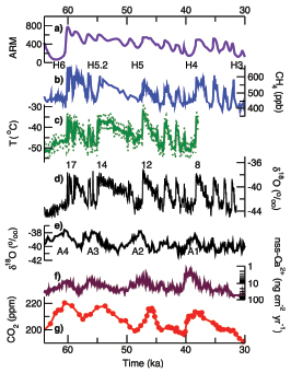
Figure 6.7. The evolution of climate indicators from the NH (panels a to d), and from Antarctica (panels e to g), over the period 64 to 30 ka. (a) Anhysteretic remanent magnetisation (ARM), here a proxy of the northward extent of Atlantic MOC, from an ocean sediment core from the Nordic Seas ( Dokken and Jansen, 1999 [PoC, JoC, SRC] ); (b) CH4 as recorded in Greenland ice cores at the Greenland Ice Core Project (GRIP), Greenland Ice Sheet Project (GISP) and North GRIP (NGRIP) sites ( Blunier and Brook, 2001 [JoC] ; Flückiger et al., 2004 [NPR, JoC] ;( Huber et al., 2006 ) ); CH4 data for the period 40 to 30 ka were selected for the GRIP site and for 64 to 40 ka for the GISP site when sample resolution is highest in the cores; (c) surface temperature estimated from nitrogen isotope ratios that are influenced by thermal diffusion ( (Huber et al., 2006 ) ); (d)d18O, a proxy for surface temperature, from NGRIP 2004 [JoC] ) with the D-O NH warm events 8, 12, 14 and 17 indicated; (e)d18Ofrom Byrd, Antarctica ( Blunier and Brook, 2001 [JoC] ) with A1 to A4 denoting antarctic warm events; (f) nss-Ca2+,a proxy of dust and iron deposition, from Dome C, Antarctica ( Röthlisberger et al., 2004 [JoC] ); and (g) CO2 as recorded in ice from Taylor Dome, Antarctica ( Indermühle et al., 2000 [JoC] ). The Heinrich events (periods of massive ice-rafted debris recorded in marine sediments) H3, H4, H5, H5.2, and H6, are shown. All data are plotted on the Greenland SS09sea time scale ( (Johnsen et al., 2001 ) ). CO2 and CH4 are well mixed in the atmosphere. CH4 variations are synchronous within the resolution of ±50 years with variations in Greenland temperature, but a detailed analysis suggests that CH4 rises lag temperature increases at the onset of the D-O events by 25 to 70 years ( (Huber et al., 2006 ) ). CO2 co-varied with the antarctic temperature, but the exact synchronisation between Taylor Dome and Byrd is uncertain, thus making the determination of leads or lags between temperature and CO2 elusive. The evolution of Greenland and antarctic temperature is consistent with a reorganisation of the heat transport and the MOC in the Atlantic ( Knutti et al., 2004 [JoC, ARC] ).
The effects of these abrupt climate changes were global, although out-of-phase responses in the two hemispheres ( Blunier et al., 1998 [JoC] ; Landais et al., 2006 [JoC] ) suggest that they were not primarily changes in global mean temperature. The highest amplitude of the changes, in terms of temperature, appears centred around the North Atlantic. Strong and fast changes are found in the global CH4 concentration (of the order of 100 to 150 ppb within decades), which may point to changes in the extent or productivity of tropical wetlands (see Chappellaz et al., 1993 [JoC, ARC] ; Brook et al., 2000 [JoC] for a review; Masson-Delmotte et al., 2005a [SRC] ), and in the Asian monsoon ( Wang et al., 2001 [JoC] ). The NH cold phases were linked with a reduced northward flow of warm waters in the Nordic Seas( Figure 6.7 ), southward shift of the Inter-Tropical Convergence Zone (ITCZ) and thus the location of the tropical rainfall belts ( Peterson et al., 2000 [JoC] ; Lea et al., 2003 [JoC] ). Cold, dry and windy conditions with low CH4 and high dust aerosol concentrations generally occurred together in the NH cold events. The accompanying changes in atmospheric CO2 content were relatively small (less than 25 ppm; Figure 6.7 )and parallel to the antarctic counterparts of Greenland D-O events. The record inN2Ois less complete and shows an increase of about 50 ppb and a decrease of about 30 ppb during warm and cold periods, respectively ( Flückiger et al., 2004 [NPR, JoC] ).
Asouthward shift of the boreal treeline and other rapid vegetation responses were associated with past cold events ( (Peteet, 1995; ) Shuman et al., 2002 [JoC] ;( Williams et al., 2002 ) ). Decadal-scale changes in vegetation have been recorded in annually laminated sequences at the beginning and the end of the Younger Dryas and the 8.2 ka event ( Birks and Ammann, 2000 [JoC] ;( Tinner and Lotter, 2001; ) ( Veski et al., 2004 ) ). Marine pollen records with a typical sampling resolution of 200 years provide unequivocal evidence of the immediate response of vegetation in Southern Europe to the climate fluctuations during glacial times ( Sánchez Goñi et al., 2002 [JoC] ; Tzedakis, 2005 [JoC] ). The same holds true for the vegetation response in northern South America during the last deglaciation ( Hughen et al., 2004 [JoC, ARC] ).
6.4.2.2 What Is Known About the Mechanism of these Abrupt Changes?
There is good evidence now from sediment data for a link between these glacial-age abrupt changes in surface climate and ocean circulation changes ( Clark et al., 2002 [JoC, ARC] ). Proxy data show that the South Atlantic cooled when the north warmed (with a possible lag), and vice versa ( Voelker, 2002 [JoC] ), a seesaw of NH and SH temperatures that indicates an ocean heat transport change ( Crowley, 1992 [PoC, JoC] ; Stocker and Johnsen 2003 [JoC, MoS, ARC] ). During D-O warming, salinity in the Irminger Sea increased strongly ( Elliot et al., 1998 [JoC] ; van Kreveld et al., 2000 [JoC] ) and northward flow of temperate waters increased in the Nordic Seas ( Dokken and Jansen, 1999 [PoC, JoC, SRC] ), indicative of saline Atlantic waters advancing northward. Abrupt changes in deep water properties of the Atlantic have been documented from proxy data (e.g., 13C, 231Pa/230Th), which reconstruct the ventilation of the deep water masses and changes in the overturning rate and flow speed of the deep waters ( Vidal et al., 1998 [JoC, SRC] ; Dokken and Jansen, 1999 [PoC, JoC, SRC] ; McManus et al., 2004 [JoC] ;( Gherardi et al., 2005 ) ). Despite this evidence, many features of the abrupt changes are still not well constrained due to a lack of precise temporal control of the sequencing and phasing of events between the surface, the deep ocean and ice sheets.
Heinrich events are thought to have been caused by ice sheet instability ( MacAyeal, 1993 [JoC, ARC] ). Iceberg discharge would have provided a large freshwater forcing to the Atlantic, which can be estimated from changes in the abundance of the isotope 18O. These yield a volume of freshwater addition typically corresponding to a few (up to 15) metres of global sea level rise occurring over several centuries (250–750 years), that is, a flux of the order of 0.1 Sv ( Hemming, 2004 [JoC] ). For Heinrich event 4, Roche et al. 2004 [JoC, MoS, SRC] ) have constrained the freshwater amount to 2 ±1 m of sea level equivalent provided by the Laurentide Ice Sheet, and the duration of the event to 250 ±150 years. Volume and timing of freshwater release is still controversial, however.
Freshwater influx is the likely cause for the cold events at the end of the last ice age (i.e., the Younger Dryas and the 8.2 ka event). Rather than sliding ice, it is the inflow of melt water from melting ice due to the climatic warming at this time that could have interfered with the MOC and heat transport in the Atlantic – a discharge into the Arctic Ocean of the order 0.1 Sv may have triggered the Younger Dryas ( Tarasov and Peltier, 2005 [JoC, MoS] ), while the 8.2 ka event was probably linked to one or more floods equal to 11 to 42 cm of sea level rise within a few years ( Clarke et al., 2004 [JoC, ARC] ; see Section 6.5.2 ). This is an important difference relative to the D-O events, for which no large forcing of the ocean is known; model simulations suggest that a small forcing may be sufficient if the ocean circulation is close to a threshold ( Ganopolski and Rahmstorf, 2001 [PoC, JoC, MoS, SRC] ). The exact cause and nature of these ocean circulation changes, however, are not universally agreed. Some authors have argued that some of the abrupt climate shifts discussed could have been triggered from the tropics (e.g., Clement and Cane, 1999 [NPR, MoS, ARC] ), but a more specific and quantitative explanation for D-O events building on this idea is yet to emerge.
Atmospheric CO2 changes during the glacial antarctic warm events, linked to changes in NADW ( Knutti et al., 2004 [JoC, ARC] ), were small (less than 25 ppm; Figure 6.7 ). A relatively small positive feedback between atmospheric CO2 and changes in the rate of NADW formation is found in palaeoclimate and global warming simulations ( Joos et al., 1999 [PoC, JoC, MoS, SRC] ; Marchal et al., 1999 [JoC, MoS] ). Thus, palaeodata and available model simulations agree that possible future changes in the NADW formation rate would have only modest effects on atmospheric CO2.This finding does not, however, preclude the possibility that circulation changes in other ocean regions, in particular in the Southern Ocean, could have a larger impact on atmospheric CO2 ( Greenblatt and Sarmiento, 2004 [NPR] ).
6.4.2.3 Can Climate Models Simulate these Abrupt Changes?
Modelling the ice sheet instabilities that are the likely cause of Heinrich events is a difficult problem because the physics are not sufficiently understood, although recent results show some promise ( Calov et al., 2002 [JoC, MoS, ARC] ). Many model studies have been performed in which an influx of freshwater from an ice sheet instability (Heinrich event) or a melt water release (8.2 ka event; see Section 6.5.2 )has been assumed and prescribed, and its effects on ocean circulation and climate have been simulated. These experiments suggest that freshwater input of the order of magnitude deduced from palaeoclimatic data could indeed have caused the Atlantic MOC to shut down, and that this is a physically viable explanation for many of the climatic repercussions found in the data (e.g., the high-latitude northern cooling, the shift in the ITCZ and the hemispheric seesaw; Vellinga and Wood, 2002 [JoC, ARC] ; Dahl et al., 2005 [JoC, MoS, ARC] ; Zhang and Delworth, 2005 [JoC, MoS, ARC] ). The phase relation between temperature in Greenland and Antarctic has been explained by a reduction in the NADW formation rate and oceanic heat transport into the North Atlantic region, producing cooling in the North Atlantic and a lagged warming in the SH ( Ganopolski and Rahmstorf, 2001 [PoC, JoC, MoS, SRC] ; Stocker and Johnsen, 2003 [JoC, MoS, ARC] ). In freshwater simulations where the North Atlantic MOC is forced to collapse, the consequences also include an increase in nutrient-rich water in the deep Atlantic Ocean, higher 231Pa/230Th ratios in North Atlantic sediments ( Marchal et al., 2000 [PoC, JoC, SRC] ), a retreat of the northern treeline ( Scholze et al., 2003 [JoC, MoS, ARC] ; Higgins, 2004 [JoC] ; Köhler et al., 2005 [PoC, JoC, MoS, SRC] ), a small (10 ppm) temporary increase in atmospheric CO2 in response to a reorganisation of the marine carbon cycle ( Marchal et al., 1999 [JoC, MoS] ) and CO2 changes of a few parts per million due to carbon stock changes in the land biosphere ( Köhler et al., 2005 [PoC, JoC, MoS, SRC] ). A 10 ppb reduction in atmosphericN2Ois found in one ocean-atmosphere model ( Goldstein et al., 2003 [NPR, PoC, JoC, MoS, SRC] ), suggesting that part of the measuredN2Ovariation (up to 50 ppb) is of terrestrial origin. In summary, model simulations broadly reproduce the observed variations during abrupt events of this type.
Dansgaard-Oeschger events appear to be associated with latitudinal shifts in oceanic convection between the Nordic Seas and the open mid-latitude Atlantic ( Alley and Clark, 1999 [ARC] ). Models suggest that the temperature evolution in Greenland, the seesaw response in the South Atlantic, the observed Irminger Sea salinity changes and other observed features of the events may be explained by such a mechanism ( Ganopolski and Rahmstorf, 2001 [PoC, JoC, MoS, SRC] ), although the trigger for the ocean circulation changes remains undetermined. Alley et al. 2001 [JoC, ARC] ) showed evidence for a stochastic resonance process at work in the timing of these events, which means that a regular cycle together with random ‘noise’ could have triggered them. This can be reproduced in models (e.g., the above), as long as a threshold mechanism is involved in causing the events.
Some authors have argued that climate models tend to underestimate the size and extent of past abrupt climate changes ( Alley et al., 2003 [JoC, ARC] ), and hence may underestimate the risk of future ones. However, such a general conclusion is probably too simple, and a case-by-case evaluation is required to understand which effects may be misinterpreted in the palaeoclimatic record and which mechanisms may be underestimated in current models. This issue is important for an assessment of risks for the future: the expected rapid warming in the coming centuries could approach the amount of warming at the end of the last glacial, and would occur at a much faster rate. Hence, melt water input from ice sheets could again become an important factor influencing the ocean circulation, as for the Younger Dryas and 8.2 ka events. A melting of the Greenland Ice Sheet (equivalent to 7 m of global sea level) over 1 kyr would contribute an average freshwater flux of 0.1 Sv; this is a comparable magnitude to the estimated freshwater fluxes associated with past abrupt climate events. Most climate models used for future scenarios have thus far not included melt water runoff from melting ice sheets. Intercomparison experiments subjecting different models to freshwater influx have revealed that while responses are qualitatively similar, the amount of freshwater needed for a shutdown of the Atlantic circulation can differ greatly between models; the reasons for this model dependency are not yet fully understood ( Rahmstorf et al., 2005 [PoC, JoC, MoS, SRC] ; Stouffer et al., 2006 [JoC, MoS, ARC] ). Given present knowledge, future abrupt climate changes due to ocean circulation changes cannot be ruled out.
6.4.3 Sea Level Variations Over the Last Glacial-Interglacial Cycle
6.4.3.1 What Is the Influence of Past Ice Volume Change on Modern Sea Level Change?
Palaeorecords of sea level history provide a crucial basis for understanding the background variations upon which the sea level rise related to modern processes is superimposed. Even if no anthropogenic effect were currently operating in the climate system, measurable and significant changes in relative sea level (RSL) would still be occurring. The primary cause of this natural variability in sea level has to do with the planet’s memory of the last deglaciation event. Through the so-called glacial isostatic adjustment (GIA) process, gravitational equilibrium is restored following deglaciation, not only by crustal ‘rebound’, but also through the horizontal redistribution of water in the ocean basins required to maintain the ocean surface at gravitational equipotential.
Models of the global GIA process have enabled isolation of a contribution to the modern rate of global sea level rise being measured by the TOPography EXperiment (TOPEX)/Poseidon (T/P) satellite of –0.28 mm yr–1 for the ICE-4G(VM2) model of Peltier 1996 [JoC] ) and –0.36 mm yr–1 for the ICE-5G(VM2) model of Peltier 2004 [MoS] ). These analyses ( Peltier, 2001 [NPR] ) imply that the impact of modern climate change on the global rate of sea level rise is larger than implied by the uncorrected T/P measurements (see also Chapter5 ).
By employing the same theory to predict the impact upon Earth’s rotational state due to both the Late Pleistocene glacial cycle and the influence of present-day melting of the great polar ice sheets on Greenland and Antarctica, it has also proven possible to estimate the extent to which these ice sheets may have been losing mass over the past century. In Peltier 1998 [JoC] ), such analysis led to an upper-bound estimate of approximately 0.5 mm yr–1 for the rate of global sea level rise equivalent to the mass loss. This suggests the plausibility of the notion that polar ice sheet and glacier melting may provide the required closure of the global sea level rise budget (see Chapters 4 and 5 ).
6.4.3.2 What Was the Magnitude of Glacial-Interglacial Sea Level Change?
Model-based palaeo-sea level analysis also helps to refine estimates of the eustatic (globally averaged) sea level rise that occurred during the most recent glacial-interglacial transition from the LGM to the Holocene. The extended coral-based RSL curve from the island of Barbados in the Caribbean Sea ( Fairbanks, 1989 [JoC] ; Peltier and Fairbanks, 2006 [JoC] ) is especially important, as the RSL history from this site has been shown to provide a good approximation to the ice-equivalent eustatic curve itself ( Peltier, 2002 [JoC] ). The fit of the prediction of the ICE-5G(VM2) model to the Fairbanks data set, as shown in Figure 6.8 b, constrains the net ice-equivalent eustatic rise subsequent to 21 ka to a value of 118.7 m, very close to the value of approximately 120 m conventionally inferred (e.g., Shackleton, 2000 [JoC] ) on the basis of deep-sea O isotopic information( Figure 6.8 b). Waelbroeck et al. 2002 [JoC, SRC] ) produced a sea level reconstruction based upon coral records and deep-sea O isotopes corrected for the influence of abyssal ocean temperature changes for the entire glacial-interglacial cycle. This record( Figure 6.8 a) is characterised by a best estimate of the LGM depression of ice-equivalent eustatic sea level that is also near 120 m. The analysis of the Red Sea O isotopic record by Siddal et al. ( 2003 ) further supports the validity of the interpretation of the extended Barbados record by Peltier and Fairbanks 2006 [JoC] ).
The ice-equivalent eustatic sea level curve of Lambeck and Chappell 2001 [JoC, ARC] ), based upon data from a variety of different sources, including the Barbados coral record, measurements from the Sunda Shelf of Indonesia ( Hanebuth et al., 2000 [JoC] ) and observations from the Bonaparte Gulf of northern Australia ( Yokoyama et al., 2000 [JoC] ), is also shown in Figure 6.8 b. This suggests an ice-equivalent eustatic sea level history that conflicts with that based upon the extended Barbados record. First, the depth of the low stand of the sea at the LGM is approximately 140 m below present sea level rather than the value of approximately 120 m required by the Barbados data set. Second, the Barbados data appear to rule out the possibility of the sharp rise of sea level at 19 ka suggested by Yokoyama et al. 2000 [JoC] ). That the predicted RSL history at Barbados using the ICE-5G(VM2) model is essentially identical to the ice-equivalent eustatic curve for the same model is shown explicitly in Figure 6.8 ,where the red curve is the model prediction and the step-discontinuous purple curve is the ice-equivalent eustatic curve.
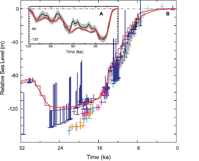
Figure 6.8. (A) The ice-equivalent eustatic sea level history over the last glacial-interglacial cycle according to the analysis of Waelbroeck et al. 2002 [JoC, SRC] ). The smooth black line defines the mid-point of their estimates for each age and the surrounding hatched region provides an estimate of error. The red line is the prediction of the ICE-5G(VM2) model for the Barbados location for which the RSL observations themselves provide an excellent approximation to the ice-equivalent eustatic sea level curve. (B) The fit of the ICE-5G(VM2) model prediction (red line) to the extended coral-based record of RSL history from the island of Barbados in the Caribbean Sea ( Fairbanks, 1989 [JoC] ; Peltier and Fairbanks, 2006 [JoC] ) over the age range from 32 ka to present. The actual ice-equivalent eustatic sea level curve for this model is shown as the step-discontinuous purple line. The individual coral-based estimates of RSL (blue) have an attached error bar that depends upon the coral species. The estimates denoted by the short error bars are derived from the Acropora palmata species, which provide the tightest constraints upon relative sea level as this species is found to live within approximately 5 m of sea level in the modern ecology. The estimates denoted by the longer error bars are derived either from the Montastrea annularis species of coral (error bars of intermediate 20 m length) or from further species that are found over a wide range of depths with respect to sea level (longest error bars). These additional data are most useful in providing a lower bound for the sea level depression. The data denoted by the coloured crosses are from the ice-equivalent eustatic sea level reconstruction of Lambeck and Chappell 2001 [JoC, ARC] ) for Barbados (cyan), Tahiti (grey), Huon (black), Bonaparte Gulf (orange) and Sunda Shelf (purple).
6.4.3.3 What Is the Significance of Higher than Present Sea Levels During the Last Interglacial Period?
The record of eustatic sea level change can be extended into the time of the LIG. Direct sea level measurements based upon coastal sedimentary deposits and tropical coral sequences (e.g., in tectonically stable settings) have clearly established that eustatic sea level was higher than present during this last interglacial by approximately 4 to 6 m (e.g., Rostami et al., 2000 [JoC, MoS] ; Muhs et al., 2002 [JoC, SRC] ). The undisturbed ice core record of the North Greenland Ice Core Project (NGRIP) to 123 ka, and older but disturbed LIG ice in the Greenland Ice Core Project (GRIP) and Greenland Ice Sheet Project 2 (GISP2) cores, indicate that the Greenland Summit region remained ice-covered during the LIG ( Raynaud et al., 1997 [JoC, SRC] ; NGRIP, 2004 [JoC] ). Similar isotopic value differences found in the Camp Century and Renland cores ( (Johnsen et al., 2001 ) ) suggest that relative elevation differences during the LIG in northern Greenland were not large ( NGRIP, 2004 [JoC] ). Interpretation of the Dye-3 ice core in southern Greenland is equivocal. The presence of isotopically enriched ice, possibly LIG ice, at the bottom of the Dye-3 core has been interpreted as substantial reduction in southern Greenland ice thickness during the LIG ( NGRIP, 2004 [JoC] ). Equally plausible interpretations suggest that the Greenland Ice Sheet’s southern dome did not survive the peak interglacial warmth and that Dye-3 is recording the growth of late-LIG ice when the ice sheet re-established itself in southern Greenland ( (Koerner and Fisher, 2002 ) ), or ice that flowed into the region from central Greenland or from a surviving but isolated southern dome (Lhomme et al., 2005a [NotFound] ). The absence of pre-LIG ice in the larger ice caps in the eastern Canadian Arctic indicates that they melted completely during the LIG ( Koerner, 1989 [JoC] ).
Most of the global sea level rise during the LIG must have been the result of polar ice sheet melting. Greenland Ice Sheet models forced with Greenland temperature scenarios derived from data ( Cuffey and Marshall, 2000 [JoC] ; Tarasov and Peltier, 2003 [JoC] ; Lhomme et al., 2005a [NotFound] ), or temperatures and precipitation produced by an AOGCM ( Otto-Bliesner et al., 2006a [PoC, JoC, MoS, SRC] ), simulate the minimal LIG Greenland Ice Sheet as a steep-sided ice sheet in central and northern Greenland( Figure 6.6 ). This inferred ice sheet, combined with the change in other arctic ice fields, likely generated no more than 2 to 4 m of early LIG sea level rise over several millennia. The simulated contribution of Greenland to this sea level rise was likely driven by orbitally forced summer warming in the Arctic (see Section 6.4.1 ). The evidence that sea level was 4 to 6 m above present implies there may also have been a contribution from Antarctica ( Scherer et al., 1998 [JoC] ; Overpeck et al., 2006 [PoC, JoC, MoS, SRC] Overpeck et al. 2006 [PoC, JoC, MoS, SRC] ) argued that since the circum-arctic LIG warming was very similar to that expected in a future doubled CO2 climate, significant retreat of the Greenland Ice Sheet can be expected to occur under this future condition. Since not all of the LIG increment of sea level appears to be explained by the melt-back of the Greenland Ice Sheet, it is possible that parts of the Antarctic Ice Sheet might also retreat under this future condition (see also Scherer et al., 1998 [JoC] ; Tarasov and Peltier, 2003 [JoC] ; Domack et al., 2005 [JoC] and Oppenheimer and Alley, 2005 [JoC, ARC] ).
6.4.3.4 What Is the Long-Term Contribution of Polar Ice-sheet Derived Melt Water to the Observed Globally Averaged Rate of Sea Level Rise?
Models of postglacial RSL history together with Holocene observations can be employed to assess whether or not a significant fraction of the observed globally averaged rate of sea level rise of about 2 mm yr–1 during the 20th century can be explained as a long term continuing influence of the most recent partial deglaciation of the polar ice sheets. Based upon post-TAR estimates derived from geological observations of Holocene sea level from 16 equatorial Pacific islands ( Peltier, 2002 [JoC] ; Peltier et al., 2002 [JoC] ), it appears likely that the average rate of sea level rise due to this hypothetical source over the last 2 kyr was zero and at most in the range 0 to 0.2 mm yr–1 ( Lambeck, 2002 [NPR, ARC] ).
6.5 The Current Interglacial
Avariety of proxy records provide detailed temporal and spatial information concerning climate change during the current interglacial, the Holocene, an approximately 11.6 kyr period of increasingly intense anthropogenic modifications of the local (e.g., land use) to global (e.g., atmospheric composition) environment. The well-dated reconstructions of the past 2 kyr are covered in Section 6.6 .In the context of both climate forcing and response, the Holocene is far better documented in terms of spatial coverage, dating and temporal resolution than previous interglacials. The evidence is clear that significant changes in climate forcing during the Holocene induced significant and complex climate responses, including long-term and abrupt changes in temperature, precipitation, monsoon dynamics and the El Niño-Southern Oscillation (ENSO). For selected periods such as the mid-Holocene, about 6 ka, intensive efforts have been dedicated to the synthesis of palaeoclimatic observations and modelling intercomparisons. Such extensive data coverage provides a sound basis to evaluate the capacity of climate models to capture the response of the climate system to the orbital forcing.
6.5.1 Climate Forcing and Response During the Current Interglacial
6.5.1.1 What Were the Main Climate Forcings During the Holocene?
During the current interglacial, changes in the Earth’s orbit modulated the latitudinal and seasonal distribution of insolation( Box 6.1 ). Ongoing efforts to quantify Holocene changes in stratospheric aerosol content recorded in the chemical composition of ice cores from both poles ( Zielinski, 2000 [JoC] ; Castellano et al., 2005 [JoC] ) confirm that volcanic forcing amplitude and occurrence varied significantly during the Holocene (see also Section 6.6.3 ). Fluctuations of cosmogenic isotopes (ice core 10Be and tree ring 14C) have been used as proxies for Holocene changes in solar activity (e.g., Bond et al., 2001 [JoC] ), although the quantitative link to solar irradiance remains uncertain and substantial work is needed to disentangle solar from non-solar influences on these proxies over the full Holocene (Muscheler et al., 2006 [NotFound] ). Residual continental ice sheets formed during the last ice age were retreating during the first half of the current interglacial period( Figure 6.8 ). The associated ice sheet albedo is thought to have locally modulated the regional climate response to the orbital forcing (e.g., Davis et al., 2003 [JoC] ).
The evolution of atmospheric trace gases during the Holocene is well known from ice core analyses( Figure 6.4 ). A first decrease in atmospheric CO2 of about 7 ppm from 11 to 8 ka was followed by a 20 ppm CO2 increase until the onset of the industrial revolution ( Monnin et al., 2004 [SRC] ). Atmospheric CH4 decreased from a NH value of about 730 ppb around 10 ka to about 580 ppb around 6 ka, and increased again slowly to 730 ppb in pre-industrial times ( Chappellaz et al., 1997 [JoC] ; Flückiger et al., 2002 [NPR, JoC] ). AtmosphericN2Olargely followed the evolution of atmospheric CO2 and shows an early Holocene decrease of about 10 ppb and an increase of the same magnitude between 8 and 2 ka ( Flückiger et al., 2002 [NPR, JoC] ). Implied radiative forcing changes from Holocene greenhouse gas variations are 0.4 Wm–2 (CO2)and 0.1 Wm–2 (N2Oand CH4), relative to pre-industrial forcing.
6.5.1.2 Why Did Holocene Atmospheric Greenhouse Gas Concentrations Vary Before the Industrial Period?
Recent transient carbon cycle-climate model simulations with a predictive global vegetation model have attributed the early Holocene CO2 decrease to forest regrowth in areas of the waning Laurentide Ice Sheet, partly counteracted by ocean sediment carbonate compensation ( Joos et al., 2004 [PoC, JoC, MoS, SRC] ). Carbonate compensation of terrestrial carbon uptake during the glacial-interglacial transition and the early Holocene, as well as coral reef buildup during the Holocene, likely contributed to the subsequent CO2 rise ( Broecker and Clark, 2003 [JoC] ; Ridgwell et al., 2003 [JoC] ; Joos et al., 2004 [PoC, JoC, MoS, SRC] ), whereas recent carbon isotope data ( Eyer, 2004 [NPR] ) and model results ( Brovkin et al., 2002 [JoC, MoS, ARC] ; Kaplan et al., 2002 [JoC, MoS] ; Joos et al., 2004 [PoC, JoC, MoS, SRC] ) suggest that the global terrestrial carbon inventory has been rather stable over the 7 kyr preceding industrialisation. Variations in carbon storage in northern peatlands may have contributed to the observed atmospheric CO2 changes. Such natural mechanisms cannot account for the much more significant industrial trace gas increases; atmospheric CO2 would be expected to remain well below 290 ppm in the absence of anthropogenic emissions ( Gerber et al., 2003 [JoC, MoS] ).
It has been hypothesised, based on Vostok ice core CO2 data ( Petit et al., 1999 [JoC] ), that atmospheric CO2 would have dropped naturally by 20 ppm during the past 8 kyr (in contrast with the observed 20 ppm increase) if prehistoric agriculture had not caused a release of terrestrial carbon and CH4 during the Holocene ( Ruddiman, 2003 [JoC] ; Ruddiman et al., 2005 [JoC] ). This hypothesis also suggests that incipient late-Holocene high-latitude glaciation was prevented by these pre-industrial greenhouse gas emissions. However, this hypothesis conflicts with several, independent lines of evidence, including the lack of orbital similarity of the three previous interglacials with the Holocene and the recent finding that CO2 concentrations were high during the entire Stage 11 ( Siegenthaler et al., 2005a [JoC] ; Figure 6.3 ), a long (~28 kyr) interglacial (see Section 6.4.1.5 ). This hypothesis also requires much larger changes in the Holocene atmospheric stable carbon isotope ratio(13C/12C) than found in ice cores ( Eyer, 2004 [NPR] ), as well as a carbon release by anthropogenic land use that is larger than estimated by comparing carbon storage for natural vegetation and present day land cover ( Joos et al., 2004 [PoC, JoC, MoS, SRC] ).
6.5.1.3 Was Any Part of the Current Interglacial Period Warmer than the Late 20th Century?
The temperature evolution over the Holocene has been established for many different regions, often with centennial-resolution proxy records more sensitive to specific seasons (see Section 6.1 ). At high latitudes of the North Atlantic and adjacent Arctic, there was a tendency for summer temperature maxima to occur in the early Holocene (10 to 8 ka), pointing to the direct influence of the summer insolation maximum on sea ice extent ( Kim et al., 2004 [JoC] ;( Kaplan and Wolfe, 2006 ) ). Climate reconstructions for the mid-northern latitudes exhibit a long-term decline in SST from the warmer early to mid-Holocene to the cooler pre-industrial period of the late Holocene ( (Johnsen et al., 2001; ) Marchal et al., 2002 [JoC] ; Andersen et al., 2004 [JoC, MoS] ; Kim et al., 2004 [JoC] ;( Kaplan and Wolfe 2006 ) ), most likely in response to annual mean and summer orbital forcings at these latitudes ( Renssen et al., 2005 [JoC, MoS, ARC] ). Near ice sheet remnants in northern Europe or North America, peak warmth was locally delayed, probably as a result of the interplay between ice elevation, albedo, atmospheric and oceanic heat transport and orbital forcing ( (MacDonald et al., 2000; ) Davis et al., 2003 [JoC] ; Kaufman et al., 2004 [JoC] ). The warmest period in northern Europe and north-western North America occurs from 7 to 5 ka ( Davis et al., 2003 [JoC] ; Kaufman et al., 2004 [JoC] ). During the mid-Holocene, global pollen-based reconstructions ( (Prentice and Webb, 1998; ) ( Prentice et al., 2000 ) ) and macrofossils ( (MacDonald et al., 2000 ) ) show a northward expansion of northern temperate forest ( Bigelow et al., 2003 [JoC] ; Kaplan et al., 2003 [NPR, JoC, MoS] ), as well as substantial glacier retreat (see Box 6.3 ). Warmer conditions at mid- and high latitudes of the NH in the early to mid-Holocene are consistent with deep borehole temperature profiles ( Huang et al., 1997 [JoC, SRC] ). Other early warm periods were identified in the equatorial west Pacific ( Stott et al., 2004 [JoC, SRC] ), China ( (He et al., 2004 ) ), New Zealand ( Williams et al., 2004 [JoC] ), southern Africa ( Holmgren et al., 2003 [JoC] ) and Antarctica ( (Masson et al., 2000 ) ). At high southern latitudes, the early warm period cannot be explained by a linear response to local summer insolation changes (see Box 6.1 ), suggesting large-scale reorganisation of latitudinal heat transport. In contrast, tropical temperature reconstructions, only available from marine records, show that Mediterranean, tropical Atlantic, Pacific and Indian Ocean SSTs exhibit a progressive warming from the beginning of the current interglacial onwards ( Kim et al., 2004 [JoC] ; Rimbu et al., 2004 [JoC, MoS] ; Stott et al., 2004 [JoC, SRC] ), possibly a reflection of tropical annual mean insolation increase( Box 6.1 ,Figure 1).
Extratropical centennial-resolution records therefore provide evidence for local multi-centennial periods warmer than the last decades by up to several degrees in the early to mid-Holocene. These local warm periods were very likely not globally synchronous and occurred at times when there is evidence that some areas of the tropical oceans were cooler than today( Figure 6.9 )(Lorenz et al., 2006 [NotFound] ). When forced by 6 ka orbital parameters, state-of-the-art coupled climate models and EMICs capture reconstructed regional temperature and precipitation changes (Sections 6.5.1.4 and 6.5.1.5 ), whereas simulated global mean temperatures remain essentially unchanged (<0.4°C; Masson-Delmotte et al., 2005b [JoC, SRC] ), just as expected from the seasonality of the orbital forcing (see Box 6.1 ). Due to different regional temperature responses from the tropics to high latitudes, as well as between hemispheres, commonly used concepts such as ‘mid-Holocene thermal optimum’, ‘altithermal’, etc. are not globally relevant and should only be applied in a well-articulated regional context. Current spatial coverage, temporal resolution and age control of available Holocene proxy data limit the ability to determine if there were multi-decadal periods of global warmth comparable to the last half of 20th century.
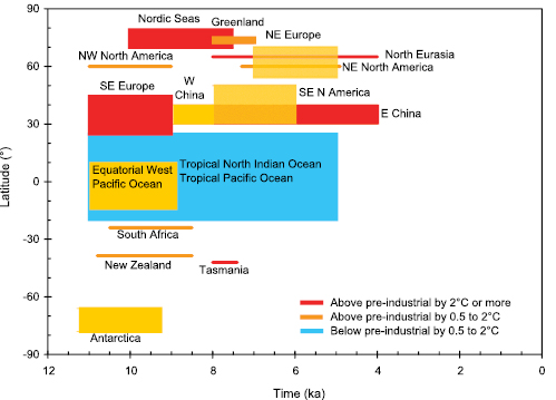
Figure 6.9. Timing and intensity of maximum temperature deviation from pre-industrial levels, as a function of latitude (vertical axis) and time (horizontal axis, in thousands of years before present ). Temperatures above pre-industrial levels by 0.5°C to 2°C appear in orange (above 2°C in red). Temperatures below pre-industrial levels by 0.5°C to 2°C appear in blue. References for data sets are: Barents Sea ( (Duplessy et al., 2001 ) ), Greenland ( (Johnsen et al., 2001 ) ), Europe ( Davis et al., 2003 [JoC] ), northwest and northeast America ( (MacDonald et al., 2000; ) Kaufman et al., 2004 [JoC] ), China ( (He et al., 2004 ) ), tropical oceans ( Rimbu et al., 2004 [JoC, MoS] ; Stott et al., 2004 [JoC, SRC] ; Lorentz et al., 2006 [NPR, JoC, MoS] ), north Atlantic ( Marchal et al., 2002 [JoC] ; Kim et al., 2004 [JoC] ), Tasmania ( (Xia et al., 2001 ) ), East Antarctica ( (Masson et al., 2000 ) ), southern Africa ( Holmgren et al., 2003 [JoC] ) and New Zealand ( Williams et al., 2004 [JoC] ).
Box 6.3: Holocene Glacier Variability
The near-global retreat of mountain glaciers is among the most visible evidence of 20th- and 21st-century climate change (see Chapter4 ), and the question arises as to the significance of this current retreat within a longer time perspective. The climatic conditions that cause an advance or a retreat may be different for glaciers located in different climate regimes (see Chapter4 ). This distinction is crucial if reconstructions of past glacier activity are to be understood properly.
Records of Holocene glacier fluctuations provide a necessary backdrop for evaluating the current global retreat. However, in most mountain regions, records documenting past glacier variations exist as discontinuous low-resolution series (see Box 6.3 ,Figure 1), whereas continuous records providing the most coherent information for the whole Holocene are available so far only in Scandinavia (e.g., Nesje et al., 2005 [NPR] ; see Box 6.3 ,Figure 1).
What do glaciers reveal about climate change during the Holocene?
Most archives from the NH and the tropics indicate short, or in places even absent, glaciers between 11 and 5 ka, whereas during the second half of the Holocene, glaciers reformed and expanded. This tendency is most probably related to changes in summer insolation due to the configuration of orbital forcing (see Box 6.1 ). Long-term changes in solar insolation, however, cannot explain the shorter, regionally diverse glacier responses, driven by complex glacier and climate (mainly precipitation and temperature) interactions. On these shorter time scales, climate phenomena such as the North Atlantic Oscillation (NAO) and ENSO affected glaciers’ mass balance, explaining some of the discrepancies found between regions. This is exemplified in the anti-phasing between glacier mass balance variations from the Alps and Scandinavia ( Reichert et al., 2001 [JoC, MoS, ARC] ;( Six et al., 2001 ) ). Comparing the ongoing retreat of glaciers with the reconstruction of glacier variations during the Holocene, no period analogous to the present with a globally homogenous trend of retreating glaciers over centennial and shorter time scales could be identified in the past, although account must be taken of the large gaps in the data coverage on retreated glaciers in most regions. This is in line with model experiments suggesting that present-day glacier retreat exceed any variations simulated by the GCM control experiments and must have an external cause, with anthropogenic forcing the most likely candidate ( Reichert et al., 2002 [JoC, ARC] ).
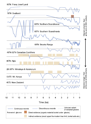
Box 6.3 ,Figure 1. Timing and relative scale of selected glacier records from both hemispheres. The different records show that Holocene glacier patterns are complex and that they should be interpreted regionally in terms of precipitation and temperature. In most cases, the scale of glacier retreat is unknown and indicated on a relative scale. Lines upper the horizontal line indicate glaciers smaller than at the end of the 20th century and lines below the horizontal line denote periods with larger glaciers than at the end of the 20th century. The radiocarbon dates are calibrated and all curves are presented in calendar years. Franz Josef Land ( Lubinski et al., 1999 [JoC] ), Svalbard from Svendsen and Mangerud 1997 [JoC] ) corrected with Humlum et al. 2005 [JoC] ), Northern Scandinavia ( (Bakke et al., 2005a, ) b; Nesje et al., 2005 [NPR] ), Southern Scandinavia ( Dahl and Nesje, 1996 [JoC] ; Matthews et al., 2000 [JoC] , 2005; Lie et al., 2004 [JoC] ), Brooks Range ( (Ellis and Calkin, 1984 ) ), Canadian Cordillera ( (Luckman and Kearney, 1986; ) Osborn and Luckman, 1988 [JoC] ;( Koch et al., 2004; ) Menounos et al., 2004 [JoC] ), Alps ( Holzhauser et al., 2005 [JoC] ; Jörin et al., 2006 [JoC, ARC] ), Himalaya and Karakorum ( (Röthlisberger and Geyh, 1985; ) Bao et al., 2003 [JoC] ), Mt. Kenya ( Karlén et al., 1999 [JoC] ), New Zealand ( Gellatly et al., 1988 [JoC] ).
6.5.1.4 What Are the Links Between Orbital Forcing and Mid-Holocene Monsoon Intensification?
Lake levels and vegetation changes reconstructed for the early to mid-Holocene indicate large precipitation increases in North Africa ( Jolly et al., 1998 [JoC, MoS] ). Simulating this intensification of the African monsoon is widely used as a benchmark for climate models within PMIP. When forced by mid-Holocene insolation resulting from changes in the Earth’s orbit (see Box 6.1 ), but fixed present-day vegetation and ocean temperatures, atmospheric models simulate NH summer continental warming and a limited enhancement of summer monsoons but underestimate the reconstructed precipitation increase and extent over the Sahara ( Joussaume et al., 1999 [JoC, MoS] ; Coe and Harrison., 2002 [JoC, MoS] ; Braconnot et al., 2004 [NPR, ARC] ). Differences among simulations appear related to atmospheric model characteristics together with the mean tropical temperature of the control simulation ( Braconnot et al., 2002 [JoC, MoS, ARC] ). As already noted in the TAR, the vegetation and surface albedo feedbacks play a major role in the enhancement of the African monsoon (e.g., Claussen and Gayler, 1997 [MoS, ARC] ; de Noblet-Ducoudre et al., 2000 [JoC, MoS] ; Levis et al., 2004 [JoC, MoS, ARC] ). New coupled ocean-atmosphere simulations show that the ocean feedback strengthens the inland monsoon flow and the length of the monsoon season, due to robust changes in late summer dipole SST patterns and in mixed layer depth ( Braconnot et al., 2004 [NPR, ARC] ; Zhao et al., 2005 [JoC, MoS] ). When combined, vegetation, soil characteristics and ocean feedbacks produce nonlinear interactions resulting in simulated precipitation in closer agreement with data ( Braconnot et al., 2000 [JoC, ARC] ; Levis et al., 2004 [JoC, MoS, ARC] ). Transient simulations of Holocene climate performed with EMICs have further shown that land surface feedbacks are possibly involved in abrupt monsoon fluctuations (see Section 6.5.2 ). The mid-Holocene intensification of the North Australian, Indian and southwest American monsoons is captured by coupled ocean-atmosphere climate models in response to orbital forcing, again with amplifying ocean feedbacks ( Harrison et al., 2003 [JoC] ; Liu et al., 2004 [NPR, MoS] ; Zhao et al., 2005 [JoC, MoS] ).
Terrestrial records of the mid-Holocene indicate an expansion of forest at the expense of tundra at mid- to high latitudes of the NH ( (MacDonald et al., 2000; ) ( Prentice et al., 2000 ) ). Since the TAR, coupled atmosphere-ocean models, including the recent PMIP-2 simulations, have investigated the response of the climate system to orbital forcing at 6 ka during the mid-Holocene( Section 6.6.1 , Box 6.1 ). Fully coupled atmosphere-ocean-vegetation models do produce the northward shift in the position of the northern limit of boreal forest, in response to simulated summer warming, and the northward expansion of temperate forest belts in North America, in response to simulated winter warming ( Wohlfahrt et al., 2004 [JoC, ARC] ). At high latitudes, the vegetation-snow albedo and ocean feedbacks enhance the warming in spring and autumn, respectively and transform the seasonal orbital forcing into an annual response ( Crucifix et al., 2002 [JoC, MoS] ; Wohlfahrt et al., 2004 [JoC, ARC] ). Ocean changes simulated for this period are generally small and difficult to quantify from data due to uncertainties in the way proxy methods respond to the seasonality and stratification of the surface waters ( Waelbroeck et al., 2005 [JoC, SRC] ). Simulations with atmosphere and slab ocean models indicate that a change in the mean tropical Pacific SSTs in the mid-Holocene to conditions more like la Niña conditions can explain North American drought conditions at mid-Holocene ( Shin et al., 2006 [JoC] ). Based on proxies of SST in the North Atlantic, it has been suggested that trends from early to late Holocene are consistent with a shift from a more meridional regime over northern Europe to a positive North Atlantic Oscillation (NAO)-like mean state in the early to mid-Holocene ( Rimbu et al., 2004 [JoC, MoS] ). A PMIP2 intercomparison shows that three of nine models support a positive NAO-like atmospheric circulation in the mean state for the mid-Holocene as compared to the pre-industrial period, without significant changes in simulated NAO variability ( Gladstone et al., 2005 [JoC, MoS] ).
6.5.1.5 What Are the Links Between Orbital Forcing and mid-Holocene Climate at Middle and High Latitudes?
6.5.1.6 Are There Long-Term Modes of Climate Variability Identified During the Holocene that Could Be Involved in the Observed Current Warming?
An increasing number of Holocene proxy records are of sufficiently high resolution to describe the climate variability on centennial to millennial time scales, and to identify possible natural quasi-periodic modes of climate variability at these time scales ( Haug et al., 2001 [JoC] ; Gupta et al., 2003 [PoC, JoC, SRC] ). Although earlier studies suggested that Holocene millennial variability could display similar frequency characteristics as the glacial variability in the North Atlantic ( Bond et al., 1997 [JoC] ), this assumption is being increasingly questioned ( Risebrobakken et al., 2003 [JoC] ; Schulz et al., 2004 [JoC, MoS, ARC] ). In many records, there is no apparent consistent pacing at specific centennial to millennial frequencies through the Holocene period, but rather shifts between different frequencies ( Moros et al., 2006 [PoC, JoC, SRC] ). The suggested synchroneity of tropical and North Atlantic centennial to millennial variability ( de Menocal et al., 2000 [JoC] ;( Mayewski et al., 2004; ) Y.J. Wang et al., 2005 [JoC] ) is not common to the SH ( (Masson et al., 2000; ) Holmgren et al., 2003 [JoC] ), suggesting that millennial scale variability cannot account for the observed 20th-century warming trend. Based on the correlation between changes in cosmogenic isotopes(10Be or 14C) – related to solar activity changes – and climate proxy records, some authors argue that solar activity may be a driver for centennial to millennial variability ( Karlén and Kuylenstierna, 1996 [JoC, MoS] ; Bond et al., 2001 [JoC] ; Fleitmann et al., 2003 [JoC, MoS, SRC] ; Y.J. Wang et al., 2005 [JoC] ). The possible importance of (forced or unforced) modes of variability within the climate system, for instance related to the deep ocean circulation, have also been highlighted ( Bianchi and McCave, 1999 [JoC] ;( Duplessy et al., 2001; ) Marchal et al., 2002 [JoC] ; Oppo et al., 2003 [JoC] ). The current lack of consistency between various data sets makes it difficult, based on current knowledge, to attribute the millennial time scale large-scale climate variations to external forcings (solar activity, episodes of intense volcanism), or to variability internal to the climate system.
The end of the first half of the Holocene – between about 5 and 4 ka – was punctuated by rapid events at various latitudes, such as an abrupt increase in NH sea ice cover ( Jennings et al., 2001 [JoC] ); a decrease in Greenland deuterium excess, reflecting a change in the hydrological cycle ( Masson-Delmotte et al., 2005b [JoC, SRC] ); abrupt cooling events in European climate ( Seppa and Birks, 2001 [JoC] ; Lauritzen, 2003 [NPR] ); widespread North American drought for centuries ( Booth et al., 2005 [JoC] ); and changes in South American climate ( (Marchant and Hooghiemstra, 2004 ) ). The processes behind these observed abrupt shifts are not well understood. As these particular events took place at the end of a local warm period caused by orbital forcing (see Box 6.1 and Section 6.5.1 ), these observations suggest that under gradual climate forcings (e.g., orbital) the climate system can change abruptly.
6.5.2 Abrupt Climate Change During the Current Interglacial
6.5.2.1 What Do Abrupt Changes in Oceanic and Atmospheric Circulation at Mid- and High-Latitudes Show?
An abrupt cooling of 2°C to 6°C identified as a prominent feature of Greenland ice cores at 8.2 ka ( Alley et al., 1997 [ARC] ; Alley and Agustsdottir, 2005 [JoC, ARC] ) is documented in Europe and North America by high-resolution continental proxy records ( (Klitgaard-Kristensen et al., 1998; ) von Grafenstein et al., 1998 [JoC] ; Barber et al., 1999 [JoC, MoS] ; Nesje et al., 2000 [JoC] ; Rohling and Palike, 2005 [JoC] ). A large decrease in atmospheric CH4 concentrations (several tens of parts per billion; Spahni et al., 2003 [JoC, SRC] ) reveals the widespread signature of the abrupt ‘8.2 ka event’ associated with large-scale atmospheric circulation change recorded from the Arctic to the tropics with associated dry episodes ( Hughen et al., 1996 [PoC, JoC, SRC] ; Stager and Mayewski, 1997 [JoC] ; Haug et al., 2001 [JoC] ; Fleitmann et al., 2003 [JoC, MoS, SRC] ; Rohling and Palike, 2005 [JoC] ). The 8.2 ka event is interpreted as resulting from a brief reorganisation of the North Atlantic MOC ( Bianchi and McCave, 1999 [JoC] ; Risebrobakken et al., 2003 [JoC] ; McManus et al., 2004 [JoC] ), however, without a clear signature identified in deep water formation records. Significant volumes of freshwater were released in the North Atlantic and Arctic at the beginning of the Holocene by the decay of the residual continental ice ( Nesje et al., 2004 [JoC] ). A likely cause for the 8.2 ka event is an outburst flood during which pro-glacial Lake Agassiz drained about 1014 m3 of freshwater into Hudson Bay extremely rapidly (possibly 5 Sv over 0.5 year; Clarke et al., 2004 [JoC, ARC] ). Climate models have been used to test this hypothesis and assess the vulnerability of the ocean and atmospheric circulation to different amounts of freshwater release (see Alley and Agustsdottir, 2005 [JoC, ARC] for a review; Section 6.4.2.2 ). Ensemble simulations conducted with EMICs ( Renssen et al., 2002 [JoC, MoS, ARC] ; Bauer et al., 2004 [JoC, MoS, SRC] ) and coupled ocean-atmosphere GCMs ( Alley and Agustsdottir, 2005 [JoC, ARC] ; LeGrande et al., 2006 ) with different boundary conditions and freshwater forcings show that climate models are capable of simulating the broad features of the observed 8.2 ka event (including shifts in the ITCZ).
6.5.2.2 What Is the Understanding of Abrupt Changes in Monsoons?
In the tropics, precipitation-sensitive records and models indicate that summer monsoons in Africa, India and Southeast Asia were enhanced in the early to mid-Holocene due to orbital forcing, a resulting increase in land-sea temperature gradients and displacement of the ITCZ. All high-resolution precipitation-sensitive records reveal that the local transitions from wetter conditions in the early Holocene to drier modern conditions occurred in one or more steps ( Guo et al., 2000 [JoC] ; Fleitmann et al., 2003 [JoC, MoS, SRC] ; Morrill et al., 2003 [PoC, JoC, SRC] ; Y.J.Wang et al., 2005 ). In the early Holocene, large increases in monsoon-related northern African runoff and/or wetter conditions over the Mediterranean are associated with dramatic changes in Mediterranean Sea ventilation, as evidenced by sapropel layers ( (Ariztegui et al., 2000 ) ).
Transient simulations of the Holocene, although usually after the final disappearance of ice sheets, have been performed with EMICs and forced by orbital parameters( Box 6.1 ). These models have pointed to the operation of mechanisms that can generate rapid events in response to orbital forcing, such as changes in African monsoon intensity due to nonlinear interactions between vegetation and monsoon dynamics ( Claussen et al., 1999 [JoC, MoS, ARC] ; Renssen et al., 2003 [Ambiguous] ).
6.5.3 How and Why Has the El Niño-Southern Oscillation Changed Over the Present Interglacial?
High-resolution palaeoclimate records from diverse sources (corals, archaeological middens, lake and ocean sediments) consistently indicate that the early to mid-Holocene likely experienced weak ENSO variability, with a transition to a stronger modern regime occurring in the past few thousand years ( Shulmeister and Lees, 1995 [JoC] ; Gagan et al., 1998 [JoC] ; Rodbell et al., 1999 [JoC] ; Tudhope et al., 2001 [JoC] ; Moy et al., 2002 [JoC] ; McGregor and Gagan, 2004 [JoC] ). Most data sources are discontinuous, providing only snapshots of mean conditions or interannual variability, and making it difficult to precisely characterise the rate and timing of the transition to the modern regime.
Asimple model of the coupled Pacific Ocean and atmosphere, forced with orbital insolation variations, suggests that seasonal changes in insolation can produce systematic changes in ENSO behaviour ( Clement et al., 1996 [JoC, ARC] , 2000; Cane, 2005 [MoS] ). This model simulates a progressive, somewhat irregular increase in both event frequency and amplitude throughout the Holocene, due to the Bjerknes feedback mechanism ( Bjerknes, 1969 [JoC] ) and ocean dynamical thermostat ( Clement and Cane, 1999 [NPR, MoS, ARC] ; Clement et al., 2001 [ARC] ; Cane, 2005 [MoS] ). Snapshot experiments conducted with some coupled GCMs also reproduce an intensification of ENSO between the early Holocene and the present, although with some disagreement as to the magnitude of change. Both model results and data syntheses suggest that before the mid-Holocene, the tropical Pacific exhibited a more la Niña-like background state ( Clement et al., 2000 [JoC, ARC] ; Liu et al., 2000 [JoC, MoS] ; Kitoh and Murakami, 2002 [JoC, MoS, ARC] ; Otto-Bliesner et al., 2003 [JoC, MoS, SRC] ; Liu, 2004 [NPR, MoS] ). In palaeoclimate simulations with GCMs, ENSO teleconnections robust in the modern system show signs of weakening under mid-Holocene orbital forcing ( Otto-Bliesner, 1999 [JoC, SRC] ; Otto-Bliesner et al., 2003 [JoC, MoS, SRC] ).
6.6 The Last 2,000 Years
6.6.1 Northern Hemisphere Temperature Variability
6.6.1.1 What Do Reconstructions Based on Palaeoclimatic Proxies Show?
Figure 6.10 shows the various instrumental and proxy climate evidence of the variations in average large-scale surface temperatures over the last 1.3 kyr. Figure 6.10 ashows two instrumental compilations representing the mean annual surface temperature of the NH since 1850, one based on land data only, and one using land and surface ocean data combined (see Chapter3 ). The uncertainties associated with one of these series are also shown (30-year smoothed combined land and marine). These arise primarily from the incomplete spatial coverage of instrumentation through time ( Jones et al., 1997 [PoC, JoC, MoS, SRC] ) and, whereas these uncertainties are larger in the 19th compared to the 20th century, the prominence of the recent warming, especially in the last two to three decades of the record, is clearly apparent in this 150-year context. The land-only record shows similar variability, although the rate of warming is greater than in the combined record after about 1980 . The land-only series can be extended back beyond the 19th century, and is shown plotted from 1781 onwards. The early section is based on a much sparser network of available station data, with at least 23 European stations, but only one North American station, spanning the first two decades, and the first Asian station beginning only in the 1820 s. Four European records (Central England, De Bilt, Berlin and Uppsala) provide an even longer, though regionally restricted, indication of the context for the warming observed in the last approximately 20 to 30 years, which is even greater in this area than is observed over the NH land as a whole.
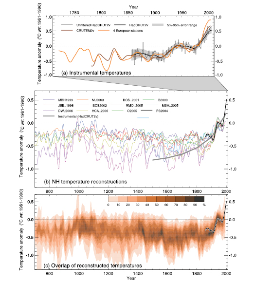
Figure 6.10. Records of NH temperature variation during the last 1.3 kyr. (a) Annual mean instrumental temperature records, identified in Table 6.1 .(b) Reconstructions using multiple climate proxy records, identified in Table 6.1 ,including three records (JBB.. 1998, MBH.. 1999 and BOS.. 2001 ) shown in the TAR, and the HadCRUT2v instrumental temperature record in black. (c) Overlap of the published multi-decadal time scale uncertainty ranges of all temperature reconstructions identified in Table 6.1 (except for RMO.. 2005 and PS 2004 ), with temperatures within ±1 standard error (SE) of a reconstruction ‘scoring’ 10%, and regions within the 5 to 95% range ‘scoring’ 5% (the maximum 100% is obtained only for temperatures that fall within ±1 SE of all 10 reconstructions). The HadCRUT2v instrumental temperature record is shown in black. All series have been smoothed with a Gaussian-weighted filter to remove fluctuations on time scales less than 30 years; smoothed values are obtained up to both ends of each record by extending the records with the mean of the adjacent existing values. All temperatures represent anomalies (°C) from the 1961 to 1990 mean.
The instrumental temperature data that exist before 1850, although increasingly biased towards Europe in earlier periods, show that the warming observed after 1980 is unprecedented compared to the levels measured in the previous 280 years, even allowing for the greater variance expected in an average of so few early data compared to the much greater number in the 20th century. Recent analyses of instrumental, documentary and proxy climate records, focussing on European temperatures, have also pointed to the unprecedented warmth of the 20th century and shown that the extreme summer of 2003 was very likely warmer than any that has occurred in at least 500 years ( Luterbacher et al., 2004 [JoC, ARC] ; Guiot et al., 2005 [JoC] ; see Box 3.6 ).
If the behaviour of recent temperature change is to be understood, and the mechanisms and causes correctly attributed, parallel efforts are needed to reconstruct the longer and more widespread pre-instrumental history of climate variability, as well as the detailed changes in various factors that might influence climate ( Bradley et al., 2003b [NPR, PoC, MoS, SRC] ; Jones and Mann, 2004 [PoC, JoC, ARC] ).
The TAR discussed various attempts to use proxy data to reconstruct changes in the average temperature of the NH for the period after AD 1000, but focused on three reconstructions (included in Figure 6.10 ), all with yearly resolution. The first ( Mann et al., 1999 [PoC, JoC] ) represents mean annual temperatures, and is based on a range of proxy types, including data extracted from tree rings, ice cores and documentary sources; this reconstruction also incorporates a number of instrumental (temperature and precipitation) records from the 18th century onwards. For 900 years, this series exhibits multi-decadal fluctuations with amplitudes up to 0.3°C superimposed on a negative trend of 0.15°C, followed by an abrupt warming (~0.4°C) matching that observed in the instrumental data during the first half of the 20th century. Of the other two reconstructions, one ( Jones et al., 1998 [PoC, JoC, MoS, SRC] ) was based on a much smaller number of proxies, whereas the other ( Briffa et al., 2001 [PoC, JoC, SRC] ) was based solely on tree ring density series from an expansive area of the extratropics, but reached back only to AD 1400 . These two reconstructions emphasise warm season rather than annual temperatures, with a geographical focus on extratropical land areas. They indicate a greater range of variability on centennial time scales prior to the 20th century, and also suggest slightly cooler conditions during the 17th century than those portrayed in the Mann et al. 1998 [PoC, JoC, MoS] , 1999 ) series.
The ‘hockey stick’ reconstruction of Mann et al. 1999 [PoC, JoC] ) has been the subject of several critical studies. ( Soon and Baliunas 2003 ) ) challenged the conclusion that the 20th century was the warmest at a hemispheric average scale. They surveyed regionally diverse proxy climate data, noting evidence for relatively warm (or cold), or alternatively dry (or wet) conditions occurring at any time within pre-defined periods assumed to bracket the so-called ‘Medieval Warm Period’ (and ‘Little Ice Age’). Their qualitative approach precluded any quantitative summary of the evidence at precise times, limiting the value of their review as a basis for comparison of the relative magnitude of mean hemispheric 20th-century warmth ( Mann and Jones, 2003 [PoC, JoC, ARC] ; Osborn and Briffa, 2006 [PoC, JoC, SRC] ). Box 6.4 provides more information on the ‘Medieval Warm Period’.
Box 6.4: Hemispheric Temperatures in the ‘Medieval Warm Period’
At least as early as the beginning of the 20th century, different authors were already examining the evidence for climate changes during the last two millennia, particularly in relation to North America, Scandinavia and Eastern Europe ( Brooks, 1922 [NPR] ). With regard to Iceland and Greenland, ( Pettersson 1914 ) ) cited evidence for considerable areas of Iceland being cultivated in the 10th century. At the same time, Norse settlers colonised areas of Greenland, while a general absence of sea ice allowed regular voyages at latitudes far to the north of what was possible in the colder 14th century. Brooks 1922 [NPR] ) described how, after some amelioration in the 15th and 16th centuries, conditions worsened considerably in the 17th century; in Iceland, previously cultivated land was covered by ice. Hence, at least for the area of the northern North Atlantic, a picture was already emerging of generally warmer conditions around the centuries leading up to the end of the first millennium, but framed largely by comparison with strong evidence of much cooler conditions in later centuries, particularly the 17th century.
( Lamb 1965 ) ) seems to have been the first to coin the phrase ‘Medieval Warm Epoch’ or ‘Little Optimum’ to describe the totality of multiple strands of evidence principally drawn from western Europe, for a period of widespread and generally warmer temperatures which he put at between AD 1000 and 1200 ( Lamb, 1982 [NPR] ). It is important to note that Lamb also considered the warmest conditions to have occurred at different times in different areas: between 950 and 1200 in European Russia and Greenland, but somewhat later, between 1150 and 1300 (though with notable warmth also in the later 900s) in most of Europe ( Lamb, 1977 [NPR, MoS] ).
Much of the evidence used by Lamb was drawn from a very diverse mixture of sources such as historical information, evidence of treeline and vegetation changes, or records of the cultivation of cereals and vines. He also drew inferences from very preliminary analyses of some Greenland ice core data and European tree ring records. Much of this evidence was difficult to interpret in terms of accurate quantitative temperature influences. Much was not precisely dated, representing physical or biological systems that involve complex lags between forcing and response, as is the case for vegetation and glacier changes. Lamb’s analyses also predate any formal statistical calibration of much of the evidence he considered. He concluded that ‘High Medieval’ temperatures were probably 1.0°C to 2.0°C above early 20th-century levels at various European locations ( Lamb, 1977 [NPR, MoS] ; Bradley et al., 2003a [PoC, JoC] ).
Alater study, based on examination of more quantitative evidence, in which efforts were made to control for accurate dating and specific temperature response, concluded that it was not possible to say anything other than ‘… in some areas of the Globe, for some part of the year, relatively warm conditions may have prevailed’ ( Hughes and Diaz, 1994 [PoC, JoC] ).
In medieval times, as now, climate was unlikely to have changed in the same direction, or by the same magnitude, everywhere (Box 6.4, Figure 1). At some times, some regions may have experienced even warmer conditions than those that prevailed throughout the 20th century (e.g., see Bradley et al., 2003a [PoC, JoC] ). Regionally restricted evidence by itself, especially when the dating is imprecise, is of little practical relevance to the question of whether climate in medieval times was globally as warm or warmer than today. Local climate variations can be dominated by internal climate variability, often the result of the redistribution of heat by regional climate processes. Only very large-scale climate averages can be expected to reflect global forcings over recent millennia ( Mann and Jones, 2003 [PoC, JoC, ARC] ; Goosse et al., 2005a [PoC, JoC, MoS, ARC] ). To define medieval warmth in a way that has more relevance for exploring the magnitude and causes of recent large-scale warming, widespread and continuous palaeoclimatic evidence must be assimilated in a homogeneous way and scaled against recent measured temperatures to allow a meaningful quantitative comparison against 20th-century warmth( Figure 6.10 ).
Anumber of studies that have attempted to produce very large spatial-scale reconstructions have come to the same conclusion: that medieval warmth was heterogeneous in terms of its precise timing and regional expression ( Crowley and Lowery, 2000 [PoC, JoC] ; Folland et al., 2001 [NPR, PoC, ARC] ; Esper et al., 2002 [PoC, JoC, SRC] ; Bradley et al., 2003a [PoC, JoC] ; Jones and Mann, 2004 [PoC, JoC, ARC] ; D’Arrigo et al., 2006 [JoC] ).
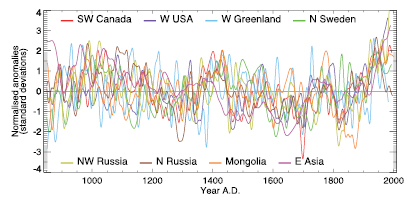
Box 6.4 ,Figure 1. The heterogeneous nature of climate during the ‘Medieval Warm Period’ is illustrated by the wide spread of values exhibited by the individual records that have been used to reconstruct NH mean temperature. These consist of individual, or small regional averages of, proxy records collated from those used by Mann and Jones 2003 [PoC, JoC, ARC] Esper et al. 2002 [PoC, JoC, SRC] and Luckman and Wilson 2005 [JoC] ), but exclude shorter series or those with no evidence of sensitivity to local temperature. These records have not been calibrated here, but each has been smoothed with a 20-year filter and scaled to have zero mean and unit standard deviation over the period 1001 to 1980 .
The uncertainty associated with present palaeoclimate estimates of NH mean temperatures is significant, especially for the period prior to 1600 when data are scarce ( Mann et al., 1999 [PoC, JoC] ; Briffa and Osborn, 2002 [PoC, JoC, SRC] ; Cook et al., 2004a [PoC, JoC, SRC] ). However, Figure 6.10 shows that the warmest period prior to the 20th century very likely occurred between 950 and 1100, but temperatures were probably between 0.1°C and 0.2°C below the 1961 to 1990 mean and significantly below the level shown by instrumental data after 1980 .
In order to reduce the uncertainty, further work is necessary to update existing records, many of which were assembled up to 20 years ago, and to produce many more, especially early, palaeoclimate series with much wider geographic coverage. There are far from sufficient data to make any meaningful estimates of global medieval warmth( Figure 6.11 ). There are very few long records with high temporal resolution data from the oceans, the tropics or the SH.
The evidence currently available indicates that NH mean temperatures during medieval times (950– 1100 ) were indeed warm in a 2-kyr context and even warmer in relation to the less sparse but still limited evidence of widespread average cool conditions in the 17th century ( Osborn and Briffa, 2006 [PoC, JoC, SRC] ). However, the evidence is not sufficient to support a conclusion that hemispheric mean temperatures were as warm, or the extent of warm regions as expansive, as those in the 20th century as a whole, during any period in medieval times ( Jones et al., 2001 [PoC, JoC, SRC] ; Bradley et al., 2003a [PoC, JoC] ,b; Osborn and Briffa, 2006 [PoC, JoC, SRC] ).
( McIntyre and McKitrick 2003 ) ) reported that they were unable to replicate the results of Mann et al. 1998 [PoC, JoC, MoS] Wahl and Ammann 2007 [NPR, PoC, JoC, ARC, 2007] ) showed that this was a consequence of differences in the way ( McIntyre and McKitrick 2003 ) ) had implemented the method of Mann et al. 1998 [PoC, JoC, MoS] ) and that the original reconstruction could be closely duplicated using the original proxy data. McIntyre and McKitrick 2005a [JoC] ,b) raised further concerns about the details of the Mann et al. 1998 [PoC, JoC, MoS] ) method, principally relating to the independent verification of the reconstruction against 19th-century instrumental temperature data and to the extraction of the dominant modes of variability present in a network of western North American tree ring chronologies, using Principal Components Analysis. The latter may have some theoretical foundation, but Wahl and Amman ( 2006 ) also show that the impact on the amplitude of the final reconstruction is very small (~0.05°C; for further discussion of these issues see also Huybers, 2005 [JoC] ; McIntyre and McKitrick, 2005c [JoC] ,d; von Storch and Zorita, 2005 [JoC, ARC] ).
Table 6.1 .Records of Northern Hemisphere temperature shown in Figure 6.10.
| Instrumental temperatures | ||||||||
|---|---|---|---|---|---|---|---|---|
| Series | Period | Description | Reference | |||||
| HadCRUT2va | 1856–2005 | Land and marine temperatures for the NH | Jones and Moberg, 2003; errors from Jones et al., 1997 | |||||
| CRUTEM2vb | 1781–2004 | Land-only temperatures for the NH | Jones and Moberg, 2003; extended using data from Jones et al., 2003 | |||||
| 4European Stations | 1721–2004 | Average of central England, De Bilt, Berlin and Uppsala | Jones et al., 2003 | |||||
| Proxy-based reconstructions of temperature | ||||||||
| Series | Period | Reconstructed Season | Region | Location Of Proxiesc | Reference | |||
| H | M | L | O | |||||
| JBB..1998 | 1000–1991 | Summer | Land, 20°N–90°N | ◢ | ◢ | □ | □ | Jones et al., 1998; calibrated by Joneset al., 2001 |
| MBH1999 | 1000–1980 | Annual | Land + marine, 0–90°N | ■ | ■ | ◢ | ◢ | Mann et al., 1999 |
| BOS..2001 | 1402–1960 | Summer | Land, 20°N–90°N | ■ | ◢ | □ | □ | Briffa et al., 2001 |
| ECS2002 | 831–1992 | Annual | Land, 20°N–90°N | ◢ | ◢ | □ | □ | Esper et al., 2002; recalibrated by Cooket al., 2004a |
| B2000 | 1–1993 | Summer | Land, 20°N–90°N | ◢ | □ | □ | □ | Briffa, 2000; calibrated by Briffa et al., 2004 |
| MJ2003 | 200–1980 | Annual | Land + marine, 0–90°N | ◢ | ◢ | □ | □ | Mann and Jones, 2003 |
| RMO..2005 | 1400–1960 | Annual | Land + marine, 0–90°N | ■ | ■ | ◢ | ◢ | Rutherford et al., 2005 |
| MSH..2005 | 1–1979 | Annual | Land + marine, 0–90°N | ◢ | ◢ | ◢ | ◢ | Moberg et al., 2005 |
| DWJ2006 | 713–1995 | Annual | Land, 20°N–90°N | ■ | ◢ | □ | □ | D’Arrigo et al., 2006 |
| HCA..2006 | 558–1960 | Annual | Land, 20°N–90°N | ◢ | ◢ | □ | □ | Hegerl et al., 2006 |
| PS2004 | 1500–2000 | Annual | Land, 0–90°N | ◢ | ■ | □ | □ | Pollack and Smerdon, 2004; reference level adjusted following Moberg et al., 2005 |
| O2005 | 1600–1990 | Summer | Global land | ◢ | ■ | □ | □ | Oerlemans, 2005 |
Since the TAR, a number of additional proxy data syntheses based on annually or near-annually resolved data, variously representing mean NH temperature changes over the last 1 or 2 kyr, have been published ( Esper et al., 2002 [PoC, JoC, SRC] ; Crowley et al., 2003 [PoC, JoC, MoS] ; Mann and Jones, 2003 [PoC, JoC, ARC] ; Cook et al., 2004a [PoC, JoC, SRC] ; Moberg et al., 2005 [JoC] ; Rutherford et al., 2005 [JoC, MoS] ; D’Arrigo et al., 2006 [JoC] ). These are shown, plotted from AD 700 in Figure 6.10 b, along with the three series from the TAR. As with the original TAR series, these new records are not entirely independent reconstructions inasmuch as there are some predictors (most often tree ring data and particularly in the early centuries) that are common between them, but in general, they represent some expansion in the length and geographical coverage of the previously available data (Figures 6.10 and 6.11 ).
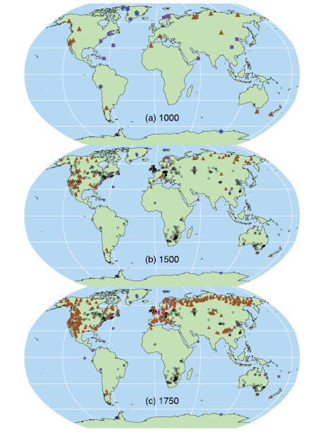
Figure 6.11. Locations of proxy records with data back to AD 1000, 1500 and 1750 (instrumental: red thermometers; tree ring: brown triangles; borehole: black circles; ice core/ice borehole: blue stars; other including low-resolution records: purple squares) that have been used to reconstruct NH or SH temperatures by studies shown in Figure 6.10 (see Table 6.1 ,excluding O 2005 ) or used to indicate SH regional temperatures (Figure 6.12).
Briffa 2000 [PoC, JoC, SRC] ) produced an extended history of interannual tree ring growth incorporating records from sites across northern Fennoscandia and northern Siberia, using a statistical technique to construct the tree ring chronologies that is capable of preserving multi-centennial time scale variability. Although ostensibly representative of northern Eurasian summer conditions, these data were later scaled using simple linear regression against a mean NH land series to provide estimates of summer temperature over the past 2 kyr ( Briffa et al., 2004 [PoC, JoC, SRC] Esper et al. 2002 [PoC, JoC, SRC] ) took tree ring data from 14 sites in Eurasia and North America, and applied a variant of the same statistical technique designed to produce ring width chronologies in which evidence of long time scale climate forcing is better represented compared with earlier tree ring processing methods. The resulting series were averaged, smoothed and then scaled so that the multi-decadal variance matched that in the Mann et al. 1998 [PoC, JoC, MoS] ) reconstruction over the period 1900 to 1977 . This produced a reconstruction with markedly cooler temperatures during the 12th to the end of the 14th century than are apparent in any other series. The relative amplitude of this reconstruction is reduced somewhat when recalibrated directly against smoothed instrumental temperatures ( Cook et al., 2004a [PoC, JoC, SRC] ) or by using annually resolved temperature data ( Briffa and Osborn, 2002 [PoC, JoC, SRC] ), but even then, this reconstruction remains at the coldest end of the range defined by all currently available reconstructions.
Mann and Jones 2003 [PoC, JoC, ARC] ) selected only eight normalised series (all screened for temperature sensitivity) to represent annual mean NH temperature change over the last 1.8 kyr. Four of these eight represent integrations of multiple proxy site records or reconstructions, including some O isotope records from ice cores and documentary information as well tree ring records. A weighted average of these decadally smoothed series was scaled so that its mean and standard deviation matched those of the NH decadal mean land and marine record over the period 1856 to 1980 Moberg et al. 2005 [JoC] ) used a mixture of tree ring and other proxy-based climate reconstructions to represent changes at short and longer time scales, respectively, across the NH. Seven tree ring series provided information on time scales shorter than 80 years, while 11 far less accurately dated records with lower resolution (including ice melt series, lake diatoms and pollen data, chemistry of marine shells and foraminifera, and one borehole temperature record from the Greenland Ice Sheet) were combined and scaled to match the mean and standard deviation of the instrumental record between 1856 and 1979 . This reconstruction displays the warmest temperatures of any reconstruction during the 10th and early 11th centuries, although still below the level of warmth observed since 1980 .
Many of the individual annually resolved proxy series used in the various reconstruction studies cited above have been combined in a new reconstruction (only back to AD 1400 ) based on a climate field reconstruction technique ( Rutherford et al., 2005 [JoC, MoS] ). This study also involved a methodological exploration of the sensitivity of the results to the precise specification of the predictor set, as well as the predictand target region and seasonal window. It concluded that the reconstructions were reasonably robust to differences in the choice of proxy data and statistical reconstruction technique.
D’Arrigo et al. 2006 [JoC] ) used only tree ring data, but these include a substantial number not used in other reconstructions, particularly in northern North America. Their reconstruction, similar to that of Esper et al. 2002 [PoC, JoC, SRC] ), displays a large amplitude of change during the past 1 kyr, associated with notably cool excursions during most of the 9th, 13th and 14th centuries, clearly below those of most other reconstructions. Hegerl et al. 2006 [PoC, JoC, ARC] ) used a mixture of 14 regional series, of which only 3 were not made up from tree ring data (a Greenland ice O isotope record and two composite series, from China and Europe, including a mixture of instrumental, documentary and other data). Many of these are common to the earlier reconstructions. However, these series were combined and scaled using a regression approach (total least squares) intended to prevent the loss of low-frequency variance inherent in some other regression approaches. The reconstruction produced lies close to the centre of the range defined by the other reconstructions.
Various statistical methods are used to convert the various sets of original palaeoclimatic proxies into the different estimates of mean NH temperatures shown in Figure 6.10 (see discussions in Jones and Mann, 2004 [PoC, JoC, ARC] ; Rutherford et al., 2005 [JoC, MoS] ). These range from simple averaging of regional data and scaling of the resulting series so that its mean and standard deviation match those of the observed record over some period of overlap ( Jones et al., 1998 [PoC, JoC, MoS, SRC] ; Crowley and Lowery, 2000 [PoC, JoC] ), to complex climate field reconstruction, where large-scale modes of spatial climate variability are linked to patterns of variability in the proxy network via a multivariate transfer function that explicitly provides estimates of the spatio-temporal changes in past temperatures, and from which large-scale average temperature changes are derived by averaging the climate estimates across the required region ( Mann et al., 1998 [PoC, JoC, MoS] ; Rutherford et al., 2003 [PoC, JoC, MoS, ARC] , 2005 ). Other reconstructions can be considered to represent what are essentially intermediate applications between these two approaches, in that they involve regionalisation of much of the data prior to the use of a statistical transfer function, and so involve fewer, but potentially more robust, regional predictors ( Briffa et al., 2001 [PoC, JoC, SRC] ; Mann and Jones, 2003 [PoC, JoC, ARC] ; D’Arrigo et al., 2006 [JoC] ). Some of these studies explicitly or implicitly reconstruct tropical temperatures based on data largely from the extratropics, and assume stability in the patterns of climate association between these regions. This assumption has been questioned on the basis of both observational and model-simulated data suggesting that tropical to extratropical climate variability can be decoupled ( Rind et al., 2005 [JoC, SRC] ), and also that extratropical teleconnections associated with ENSO may vary through time (see Section 6.5.6).
Oerlemans 2005 [JoC, ARC] ) constructed a temperature history for the globe based on 169 glacier length records. He used simplified glacier dynamics that incorporate specific response time and climate sensitivity estimates for each glacier. The reconstruction suggests that moderate global warming occurred after the middle of the 19th century, with about 0.6°C warming by the middle of the 20th century. Following a 25-year cooling, temperatures rose again after 1970, though much regional and high-frequency variability is superimposed on this overall interpretation. However, this approach does not allow for changing glacier sensitivity over time, which may limit the information before 1900 . For example, analyses of glacier mass balances, volume changes and length variations along with temperature records in the western European Alps ( (Vincent et al., 2005 ) ) indicate that between 1760 and 1830, glacier advance was driven by precipitation that was 25% above the 20th century average, while there was little difference in average temperatures. Glacier retreat after 1830 was related to reduced winter precipitation and the influence of summer warming only became effective at the beginning of the 20th century. In southern Norway, early 18th-century glacier advances can be attributed to increased winter precipitation rather than cold temperatures ( Nesje and Dahl, 2003 [JoC] ).
Changes in proxy records, either physical (such as the isotopic composition of various elements in ice) or biological (such as the width of a tree ring or the chemical composition of a growth band in coral), do not respond precisely or solely to changes in any specific climate parameter (such as mean temperature or total rainfall), or to the changes in that parameter as measured over a specific ‘season’ (such as June to August or January to December). For this reason, the proxies must be ‘calibrated’ empirically, by comparing their measured variability over a number of years with available instrumental records to identify some optimal climate association, and to quantify the statistical uncertainty associated with scaling proxies to represent this specific climate parameter. All reconstructions, therefore, involve a degree of compromise with regard to the specific choice of ‘target’ or dependent variable. Differences between the temperature reconstructions shown in Figure 6.10 bare to some extent related to this, as well as to the choice of different predictor series (including differences in the way these have been processed). The use of different statistical scaling approaches (including whether the data are smoothed prior to scaling, and differences in the period over which this scaling is carried out) also influences the apparent spread between the various reconstructions. Discussions of these issues can also be found in Harris and Chapman 2001 [JoC] Beltrami 2002 [JoC] Briffa and Osborn 2002 [PoC, JoC, SRC] Esper et al. 2002 [PoC, JoC, SRC] Trenberth and Otto-Bliesner 2003 [PoC, JoC, SRC] Zorita et al. 2003 [JoC, MoS, ARC] Jones and Mann 2004 [PoC, JoC, ARC] Pollack and Smerdon 2004 [JoC, SRC] Esper et al. 2005 [PoC, JoC, SRC] and Rutherford et al. 2005 [JoC, MoS] ).
The considerable uncertainty associated with individual reconstructions (2-standard-error range at the multi-decadal time scale is of the order of ±0.5°C) is shown in several publications, calculated on the basis of analyses of regression residuals ( Mann et al., 1998 [PoC, JoC, MoS] ; Briffa et al., 2001 [PoC, JoC, SRC] ; Jones et al., 2001 [PoC, JoC, SRC] ; Gerber et al., 2003 [JoC, MoS] ; Mann and Jones, 2003 [PoC, JoC, ARC] ; Rutherford et al., 2005 [JoC, MoS] ; D’Arrigo et al., 2006 [JoC] ). These are often calculated from the error apparent in the calibration of the proxies. Hence, they are likely to be minimum uncertainties, as they do not take into account other sources of error not apparent in the calibration period, such as any reduction in the statistical robustness of the proxy series in earlier times ( Briffa and Osborn, 1999 [PoC, JoC, SRC] ; Esper et al., 2002 [PoC, JoC, SRC] ; Bradley et al., 2003b [NPR, PoC, MoS, SRC] ; Osborn and Briffa, 2006 [PoC, JoC, SRC] ).
All of the large-scale temperature reconstructions discussed in this section, with the exception of the borehole and glacier interpretations, include tree ring data among their predictors so it is pertinent to note several issues associated with them. The construction of ring width and ring density chronologies involves statistical processing designed to remove non-climate trends that could obscure the evidence of climate that they contain. In certain situations, this process may restrict the extent to which a chronology portrays the evidence of long time scale changes in the underlying variability of climate that affected the growth of the trees; in effect providing a high-pass filtered version of past climate. However, this is generally not the case for chronologies used in the reconstructions illustrated in Figure 6.10 .Virtually all of these used chronologies or tree ring climate reconstructions produced using methods that preserve multi-decadal and centennial time scale variability. As with all biological proxies, the calibration of tree ring records using linear regression against some specific climate variable represents a simplification of what is inevitably a more complex and possibly time-varying relationship between climate and tree growth. That this is a defensible simplification, however, is shown by the general strength of many such calibrated relationships, and their significant verification using independent instrumental data. There is always a possibility that non-climate factors, such as changing atmospheric CO2 or soil chemistry, might compromise the assumption of uniformity implicit in the interpretation of regression-based climate reconstructions, but there remains no evidence that this is true for any of the reconstructions referred to in this assessment. A group of high-elevation ring width chronologies from the western USA that show a marked growth increase during the last 100 years, attributed by LaMarche et al. ( 1984 ) to the fertilizing effect of increasing atmospheric CO2,were included among the proxy data used by Mann et al. 1998 [PoC, JoC, MoS] , 1999 ). However, their tree ring data from the western USA were adjusted specifically in an attempt to mitigate this effect. Several analyses of ring width and ring density chronologies, with otherwise well-established sensitivity to temperature, have shown that they do not emulate the general warming trend evident in instrumental temperature records over recent decades, although they do track the warming that occurred during the early part of the 20th century and they continue to maintain a good correlation with observed temperatures over the full instrumental period at the interannual time scale ( Briffa et al., 2004 [PoC, JoC, SRC] ; D’Arrigo, 2006 [JoC] ). This ‘divergence’ is apparently restricted to some northern, high-latitude regions, but it is certainly not ubiquitous even there. In their large-scale reconstructions based on tree ring density data, Briffa et al. 2001 [PoC, JoC, SRC] ) specifically excluded the post- 1960 data in their calibration against instrumental records, to avoid biasing the estimation of the earlier reconstructions (hence they are not shown in Figure 6.10 ), implicitly assuming that the ‘divergence’ was a uniquely recent phenomenon, as has also been argued by Cook et al. 2004a [PoC, JoC, SRC] ). Others, however, argue for a breakdown in the assumed linear tree growth response to continued warming, invoking a possible threshold exceedance beyond which moisture stress now limits further growth ( D’Arrigo et al., 2004 [JoC] ). If true, this would imply a similar limit on the potential to reconstruct possible warm periods in earlier times at such sites. At this time there is no consensus on these issues (for further references see NRC, 2006 [NPR] ) and the possibility of investigating them further is restricted by the lack of recent tree ring data at most of the sites from which tree ring data discussed in this chapter were acquired.
Figure 6.10 billustrates how, when viewed together, the currently available reconstructions indicate generally greater variability in centennial time scale trends over the last 1 kyr than was apparent in the TAR. It should be stressed that each of the reconstructions included in Figure 6.10 bis shown scaled as it was originally published, despite the fact that some represent seasonal and others mean annual temperatures. Except for the borehole curve ( Pollack and Smerdon, 2004 [JoC, SRC] ) and the interpretation of glacier length changes ( Oerlemans, 2005 [JoC, ARC] ), they were originally also calibrated against different instrumental data, using a variety of statistical scaling approaches. For all these reasons, these reconstructions would be expected to show some variation in relative amplitude.
Figure 6.10 cis a schematic representation of the most likely course of hemispheric mean temperature change during the last 1.3 kyr based on all of the reconstructions shown in Figure 6.10 b, and taking into account their associated statistical uncertainty. The envelopes that enclose the two standard error confidence limits bracketing each reconstruction have been overlain (with greater emphasis placed on the area within the 1 standard error limits) to show where there is most agreement between the various reconstructions. The result is a picture of relatively cool conditions in the 17th and early 19th centuries and warmth in the 11th and early 15th centuries, but the warmest conditions are apparent in the 20th century. Given that the confidence levels surrounding all of the reconstructions are wide, virtually all reconstructions are effectively encompassed within the uncertainty previously indicated in the TAR. The major differences between the various proxy reconstructions relate to the magnitude of past cool excursions, principally during the 12th to 14th, 17th and 19th centuries. Several reconstructions exhibit a short-lived maximum just prior to AD 1000 but only one ( Moberg et al., 2005 [JoC] ) indicates persistent hemispheric-scale conditions (i.e., during AD 990 to 1050 and AD 1080 to 1120 ) that were as warm as those in the 1940 s and 50s. However, the long time scale variability in this reconstruction is determined by low-resolution proxy records that cannot be rigorously calibrated against recent instrumental temperature data ( Mann et al., 2005b [PoC, JoC, ARC] ). None of the reconstructions in Fig. 6.10 show pre-20th century temperatures reaching the levels seen in the instrumental temperature record for the last two decades of the 20th century.
It is important to recognise that in the NH as a whole there are few long and well-dated climate proxies, particularly for the period prior to the 17th century( Figure 6.11 ). Those that do exist are concentrated in extratropical, terrestrial locations, and many have greatest sensitivity to summer rather than winter (or annual) conditions. Changes in seasonality probably limit the conclusions that can be drawn regarding annual temperatures derived from predominantly summer-sensitive proxies ( Jones et al., 2003 [Ambiguous] ). There are very few strongly temperature-sensitive proxies from tropical latitudes. Stable isotope data from high-elevation ice cores provide long records and have been interpreted in terms of past temperature variability ( Thompson, 2000 [Ambiguous] ), but recent calibration and modelling studies in South America and southern Tibet ( Hoffmann et al., 2003 [JoC] ; Vuille and Werner, 2005 [JoC, MoS] ; Vuille et al., 2005 [Ambiguous] ) indicate a dominant sensitivity to precipitation changes, at least on seasonal to decadal time scales, in these regions. Very rapid and apparently unprecedented melting of tropical ice caps has been observed in recent decades ( Thompson et al., 2000 [Ambiguous] ; Thompson, 2001 [NPR, SRC] ; see Box 6.3 ), likely associated with enhanced warming at high elevations ( Gaffen et al., 2000 [JoC] ; see Chapter4 ). Coral O isotopes and Sr/Ca ratios reflect SSTs, although the former are also influenced by salinity changes associated with precipitation variability ( (Lough, 2004 ) ). Unfortunately, these records are invariably short, of the order of centuries at best, and can be associated with age uncertainties of 1 or 2%. Virtually all coral records currently available from the tropical Indo-Pacific indicate unusual warmth in the 20th century ( Cole, 2003 [JoC, SRC] ), and in the tropical Indian Ocean many isotope records show a trend towards warmer conditions ( Charles et al., 1997 [JoC] ;( Kuhnert et al., 1999; ) Cole et al., 2000 [JoC, MoS, SRC] ). In most multi-centennial length coral series, the late 20th century is warmer than any time in the last 100 to 300 years.
Using pseudo-proxy networks extracted from GCM simulations of global climate for the last millennium, von Storch et al. 2004 [JoC] ) suggested that temperature reconstructions may not fully represent variance on long time scales. This would represent a bias, as distinct from the random error represented by published reconstruction uncertainty ranges. At present, the extent of any such biases in specific reconstructions and as indicated by pseudo-proxy studies is uncertain (being dependent on the choice of statistical regression model and climate model simulation used to provide the pseudo-proxies). It is very unlikely, however, that any bias would be as large as the factor of two suggested by von Storch et al. 2004 [JoC] ) with regard to the reconstruction by Mann et al. 1998 [PoC, JoC, MoS] ), as discussed by Burger and Cubash ( 2005 and Wahl et al. 2006 [PoC, JoC, ARC] ). However, the bias will depend on the degree to which past climate departs from the range of temperatures encompassed within the calibration period data ( Mann et al., 2005b [PoC, JoC, ARC] ; Osborn and Briffa, 2006 [PoC, JoC, SRC] ) and on the proportions of temperature variability occurring on short and long time scales ( Osborn and Briffa, 2004 [PoC, JoC, SRC] ). In any case, this bias would act to damp the amplitude of reconstructed departures that are further from the calibration period mean, so that temperatures during cooler periods may have been colder than estimated by some reconstructions, while periods with comparable temperatures (e.g., possible portions of the period between AD 950 and 1150, Figure 6.10 )would be largely unbiased. As only one reconstruction ( Moberg et al., 2005 [JoC] ) shows an early period that is noticeably warmer than the mean for the calibration period, the possibility of a bias does not affect the general conclusion about the relative warmth of the 20th century based on these data.
The weight of current multi-proxy evidence, therefore, suggests greater 20th-century warmth, in comparison with temperature levels of the previous 400 years, than was shown in the TAR. On the evidence of the previous and four new reconstructions that reach back more than 1 kyr, it is likely that the 20th century was the warmest in at least the past 1.3 kyr. Considering the recent instrumental and longer proxy evidence together, it is very likely that average NH temperatures during the second half of the 20th century were higher than for any other 50-year period in the last 500 years. Greater uncertainty associated with proxy-based temperature estimates for individual years means that it is more difficult to gauge the significance, or precedence, of the extreme warm years observed in the recent instrumental record, such as 1998 and 2005, in the context of the last millennium.
6.6.1.2 What Do Large-Scale Temperature Histories from Subsurface Temperature Measurements Show?
Hemispheric or global ground surface temperature (GST) histories reconstructed from measurements of subsurface temperatures in continental boreholes have been presented by several geothermal research groups ( Huang et al., 2000 [JoC, SRC] ; Harris and Chapman, 2001 [JoC] ; Beltrami, 2002 [JoC] ;( Beltrami and Bourlon, 2004; ) Pollack and Smerdon, 2004 [JoC, SRC] ); see Pollack and Huang 2000 [SRC] ) for a review of this methodology. These borehole reconstructions have been derived using the contents of a publicly available database of borehole temperatures and climate reconstructions ( Huang and Pollack, 1998 [NPR, SRC] ) that in 2004 included 695 sites in the NH and 166 in the SH( Figure 6.11 ). Because the solid Earth acts as a low-pass filter on downward-propagating temperature signals, borehole reconstructions lack annual resolution; accordingly they typically portray only multi-decadal to centennial changes. These geothermal reconstructions provide independent estimates of surface temperature history with which to compare multi-proxy reconstructions. Figure 6.10 bshows a reconstruction of average NH GST by Pollack and Smerdon 2004 [JoC, SRC] ). This reconstruction, very similar to that presented by Huang et al. 2000 [JoC, SRC] ), shows an overall warming of the ground surface of about 1.0°C over the past five centuries. The two standard error uncertainties for their series (not shown here) are 0.20°C (in 1500 ), 0.10°C ( 1800 ) and 0.04°C ( 1900 ). These are errors associated with various scales of areal weighting and consequent suppression of site-specific noise through aggregation ( Pollack and Smerdon, 2004 [JoC, SRC] ). The reconstruction is similar to the cooler multi-proxy reconstructions in the 16th and 17th centuries, but sits in the middle of the multi-proxy range in the 19th and early 20th centuries. A geospatial analysis by Mann et al. 2003 [PoC, JoC] ; see correction by Rutherford and Mann, 2004 [PoC, JoC] ) of the results of Huang et al. 2000 [JoC, SRC] ) argued for significantly less overall warming, a conclusion contested by Pollack and Smerdon 2004 [JoC, SRC] ( and Beltrami and Bourlon 2004 ) ). Geothermal reconstructions based on the publicly available database generally yield somewhat muted estimates of the 20th-century trend, because of a relatively sparse representation of borehole data north of 60°N. About half of the borehole sites at the time of measurement had not yet been exposed to the significant warming of the last two decades of the 20th century ( Taylor et al., 2006 [JoC] ;( Majorowicz et al., 2004 ) ).
The assumption that the reconstructed GST history is a good representation of the surface air temperature (SAT) history has been examined with both observational data and model studies. Observations of SAT and GST display differences at daily and seasonal time scales, and indicate that the coupling of SAT and GST over a single year is complex ( Sokratov and Barry, 2002 [JoC, ARC] ; Stieglitz et al., 2003 [JoC] ; Bartlett et al., 2004 [JoC] ; Smerdon et al., 2006 [JoC] ). The mean annual GST differs from the mean annual SAT in regions where there is snow cover and/or seasonal freezing and thawing ( Gosnold et al., 1997 [JoC] ; Smerdon et al., 2004 [JoC] ; Taylor et al., 2006 [JoC] ), as well as in regions without those effects ( Smerdon et al., 2006 [JoC] ). Observational time series of ground temperatures are not long enough to establish whether the mean annual differences are stable over long time scales. The long-term coupling between SAT and GST has been addressed by simulating both air and soil temperatures in global three-dimensional coupled climate models. Mann and Schmidt 2003 [PoC, JoC, ARC] ), in a 50-year experiment using the GISS Model E, suggested that GST reconstructions may be biased by seasonal influences and snow cover variability, an interpretation contested by Chapman et al 2004 [JoC] ). Thousand-year simulations by González-Rouco et al. 2003 [JoC, MoS, ARC] , 2006 ) using the ECHO-G model suggest that seasonal differences in coupling are of little significance over long time scales. They also indicate that deep soil temperature is a good proxy for the annual SAT on continents and that the spatial array of borehole locations is adequate to reconstruct the NH mean SAT. Neither of these climate models included time-varying vegetation cover.
6.6.2 Southern Hemisphere Temperature Variability
There are markedly fewer well-dated proxy records for the SH compared to the NH( Figure 6.11 ), and consequently little evidence of how large-scale average surface temperatures have changed over the past few thousand years. Mann and Jones 2003 [PoC, JoC, ARC] ) used only three series to represent annual mean SH temperature change over the last 1.5 kyr. A weighted combination of the individual standardised series was scaled to match (at decadal time scales) the mean and the standard deviation of SH annual mean land and marine temperatures over the period 1856 to 1980 . The recent proxy-based temperature estimates, up to the end of the reconstruction in 1980, do not capture the full magnitude of the warming seen in the instrumental temperature record. Earlier periods, around AD 700 and 1000, are reconstructed as warmer than the estimated level in the 20th century, and may have been as warm as the measured values in the last 20 years. The paucity of SH proxy data also means that uncertainties associated with hemispheric temperature estimates are much greater than for the NH, and it is more appropriate at this time to consider the evidence in terms of limited regional indicators of temperature change( Figure 6.12 ).
The long-term oscillations in warm-season temperatures shown in a tree ring reconstruction for Tasmania ( Cook et al., 2000 [PoC, JoC, SRC] ) suggest that the last 30 years was the warmest multi-decadal period in the last 1 kyr, but only by a marginal degree. Conditions were generally warm over a longer period from 1300 to 1500 ( Figure 6.12 ). Another tree ring reconstruction, of austral summer temperatures based on data from South Island, New Zealand, spans the past 1.1 kyr and is the longest yet produced for the region ( Cook et al., 2002a [PoC, JoC, SRC] ). Disturbance at the site from which the trees were sampled restricts the calibration of this record to the 70 years up until 1950, but both tree rings and instrumental data indicate that the 20th century was not anomalously warm when compared to several warm periods reconstructed in the last 1 kyr (around the mid-12th and early 13th centuries and around 1500 ).
Tree-ring based temperature reconstructions across the Southern Andes (37°S to 55°S) of South America indicate that the annual temperatures during the 20th century have been anomalously high in the context of the past four centuries. The mean annual temperatures for northern and southern Patagonia during the interval 1900 to 1990 are 0.53°C and 0.86°C above the 1640 to 1899 means, respectively( Figure 6.12 ). In Northern Patagonia, the highest temperatures occurred in the 1940 s. In Southern Patagonia, the year 1998 was the warmest of the past four centuries. The rate of temperature increase from 1850 to 1920 was the highest over the past 360 years ( Villalba et al., 2003 [JoC, SRC] ).
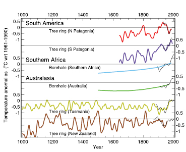
Figure 6.12. Temperature reconstructions for regions in the SH: two annual temperature series from South American tree ring data ( Villalba et al., 2003 [JoC, SRC] ); annual temperature estimates from borehole inversions for southern Africa and Australia ( Huang et al, 2000 [JoC, SRC] ); summer temperature series from Tasmania and New Zealand tree ring data ( Cook et al., 2000 [PoC, JoC, SRC] , 2002a ). The black curves show summer or annual instrumental temperatures for each region. All tree ring and instrumental series were smoothed with a 25-year filter and represent anomalies (°C) from the 1961 to 1990 mean (indicated by the horizontal lines).
Figure 6.12 also shows the evidence of GST changes over the last 500 years, provided by regionally aggregated borehole temperature inversions( Figure 6.11 )from southern Africa (92 records) and Australia (57 records) described in Huang et al. 2000 [JoC, SRC] ). The instrumental records for these areas show warmer conditions that postdate the time when the boreholes were logged; thus, the most recent warming is not registered in these borehole curves. A more detailed analysis of the Australian geothermal reconstruction ( Pollack et al., 2006 [SRC] ), indicates that the warming of Australia in the past five centuries was apparently only half that experienced over the continents of the NH during the same period and shows good correspondence with the tree-ring based reconstructions for Tasmania and New Zealand ( Cook et al., 2000 [PoC, JoC, SRC] , 2002a ). Contrasting evidence of past temperature variations at Law Dome, Antarctica has been derived from ice core isotope measurements and from the inversion of a subsurface temperature profile ( Dahl-Jensen et al., 1999 [MoS] ; Goosse et al., 2004 [JoC, MoS, ARC] ; Jones and Mann, 2004 [PoC, JoC, ARC] ). The borehole analysis indicates colder intervals at around 1250 and 1850, followed by a gradual warming of 0.7°C to the present. The isotope record indicates a relatively cold 20th century and warmer conditions throughout the period 1000 to 1750 .
Taken together, the very sparse evidence for SH temperatures prior to the period of instrumental records indicates that unusual warming is occurring in some regions. However, more proxy data are required to verify the apparent warm trend.
6.6.3 Comparisons of Millennial Simulations with Palaeodata
Arange of increasingly complex climate models has been used to simulate NH temperatures over the last 500 to 1,000 years using both natural and anthropogenic forcings( Figure 6.13 ). These models include an energy balance formulation ( Crowley et al., 2003 [PoC, JoC, MoS] , Gerber et al., 2003 [JoC, MoS] ), two- and three-dimensional reduced complexity models ( Bertrand et al., 2002b [JoC, SRC] ; Bauer et al., 2003 [JoC, MoS, SRC] ), and three fully coupled AOGCMs ( Ammann et al., 2003 [PoC, JoC, MoS, ARC] ; von Storch et al., 2004 [JoC] ; Tett et al., 2007 [JoC, MoS, ARC, 2007] ).
Comparison and evaluation of the output from palaeoclimate simulations is complicated by their use of different historical forcings, as well as by the way indirect evidence of the history of various forcings is translated into geographically and seasonally specific radiative inputs within the models. Some factors, such as orbital variations of the Earth in relation to the Sun, can be calculated accurately (e.g., Berger, 1977 [ARC] ; Bradley et al., 2003b [NPR, PoC, MoS, SRC] ) and directly implemented in terms of latitudinal and seasonal changes in incoming shortwave radiation at the top of the atmosphere. For the last 2 kyr, although this forcing is incorporated in most models, its impact on climate can be neglected compared to the other forcings ( Bertrand et al., 2002b [JoC, SRC] ).
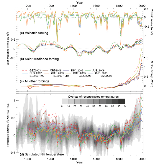
Figure 6.13. Radiative forcings and simulated temperatures during the last 1.1 kyr. Global mean radiative forcing (Wm–2)used to drive climate model simulations due to (a) volcanic activity, (b) solar irradiance variations and (c) all other forcings (which vary between models, but always include greenhouse gases, and, except for those with dotted lines after 1900, tropospheric sulphate aerosols). (d) Annual mean NH temperature (°C) simulated under the range of forcings shown in (a) to (c), compared with the concentration of overlapping NH temperature reconstructions (shown by grey shading, modified from Figure 6.10c to account for the 1500 to 1899 reference period used here). All forcings and temperatures are expressed as anomalies from their 1500 to 1899 means and then smoothed with a Gaussian-weighted filter to remove fluctuations on time scales less than 30 years; smoothed values are obtained up to both ends of each record by extending the records with the mean of the adjacent existing values. The individual series are identified in Table 6.2 .
Table 6.2 .Climate model simulations shown in Figure 6.13.
| Series | Modela | Model type | Forcingsb | Reference |
|---|---|---|---|---|
| GSZ2003 | ECHO-G | GCM | SV -G - - - - | González-Rouco et al., 2003 |
| ORB2006 | ECHO-G/MAGICC | GCM adj. using EBMc | SV -G -A -Z | Osborn et al., 2006 |
| TBC..2006 | HadCM3 | GCM | SVOG -ALZ | Tett et al., 2007 |
| AJS..2006 | NCAR CSM | GCM | SV -G -A -Z | Mann et al., 2005b |
| BLC..2002 | MoBiDiC | EMIC | SV -G -AL - | Bertrand et al., 2002b |
| CBK..2003 | - | EBMc | SV -G -A - - | Crowley et al., 2003 |
| GRT..2005 | ECBilt-CLIO | EMIC | SV -G -A - - | Goosse et al., 2005b |
| GJB..2003 | Bern CC | EBMc | SV -G -A -Z | Gerber et al., 2003 |
| B..03-14C | Climber2 | EMIC (solar from 14C) | SV - -C -L - | Bauer et al., 2003 |
| B..03-10Be | Climber2 | EMIC (solar from 10Be) | SV - -C -L - | Bauer et al., 2003 |
| GBZ..2006 | ECHO-G | GCM | SV -G - - - - | González-Rouco et al., 2006 |
| SMC2006 | ECHAM4/OPYC3 | GCM | SV -G -A -Z | Stendel et al., 2006 |
Over recent millennia, the analysis of the gas bubbles in ice cores with high deposition rates provides good evidence of greenhouse gas changes at near-decadal resolution( Figure 6.4 ). Other factors, such as land use changes ( Ramankutty and Foley, 1999 [JoC, MoS, ARC] ) and the concentrations and distribution of tropospheric aerosols and ozone, are not as well known ( Mickley et al., 2001 [JoC, MoS, SRC] ). However, because of their magnitude, uncertainties in the history of solar irradiance and volcanic effects are more significant for the pre-industrial period.
6.6.3.1 Solar Forcing
The direct measurement of solar irradiance by satellite began less than 30 years ago, and over this period only very small changes are apparent (0.1% between the peak and trough of recent sunspot cycles, which equates to only about 0.2 Wm–2 change in radiative forcing; Fröhlich and Lean 2004 [ARC] ); see Section 2.7 ). Earlier extensions of irradiance change used in most model simulations are estimated by assuming a direct correlation with evidence of changing sunspot numbers and cosmogenic isotope production as recorded in ice cores(10Be) and tree rings(14C) ( Lean et al., 1995 [JoC, ARC] ; Crowley, 2000 [PoC, JoC] ).
There is general agreement in the evolution of the different proxy records of solar activity such as cosmogenic isotopes, sunspot numbers or aurora observations, and the annually resolved records clearly depict the well-known 11-year solar cycle (Muscheler et al., 2006 [NotFound] ). For example, palaeoclimatic 10Be and 14Cvalues are higher during times of low or absent sunspot numbers. During these periods, their production is high as the shielding of the Earth’s atmosphere from cosmic rays provided by the Sun’s open magnetic field is weak ( (Beer et al., 1998 ) ). However, the relationship between the isotopic records indicative of the Sun’s open magnetic field, sunspot numbers and the Sun’s closed magnetic field or energy output are not fully understood ( Wang and Sheeley, 2003 [MoS] ).
The cosmogenic isotope records have been linearly scaled to estimate solar energy output ( Bard et al., 2000 [JoC, SRC] ) in many climate simulations. More recent studies utilise physics-based models to estimate solar activity from the production rate of cosmogenic isotopes taking into account nonlinearities between isotope production and the Sun’s open magnetic flux and variations in the geomagnetic field ( Solanki et al., 2004 [JoC, ARC] ; Muscheler et al., 2005 [PoC, JoC, SRC] ). Following this approach, Solanki et al. 2004 [JoC, ARC] ) suggested that the current level of solar activity has been without precedent over the last 8 kyr. This is contradicted by a more recent analysis linking the isotope proxy records to instrumental data that identifies, for the last millennium, three periods (around AD 1785, 1600 and 1140 ) when solar activity was as high, or higher, than in the satellite era (Muscheler et al., 2006 [NotFound] ).
The magnitude of the long-term trend in solar irradiance remains uncertain. A reassessment of the stellar data ( (Hall and Lockwood, 2004 ) ) has been unable to confirm or refute the analysis by Baliunas and Jastrow 1990 [JoC] ) that implied significant long-term solar irradiance changes, and also underpinned some of the earlier reconstructions (see Section 2.7 ). Several new studies ( Lean et al., 2002 [JoC, MoS, ARC] ; Foster, 2004 [NPR] ; Foukal et al., 2004 [PoC, JoC, ARC] ; Y.M. Wang et al., 2005 [JoC] ) suggest that long-term irradiance changes were notably less than in earlier reconstructions ( Hoyt and Schatten, 1993 [JoC] ; Lean et al., 1995 [JoC, ARC] ; Lockwood and Stamper, 1999 [JoC] ; Bard et al., 2000 [JoC, SRC] ; Fligge and Solanki, 2000 [JoC, ARC] ; Lean, 2000 [JoC, ARC] ) that were employed in a number of TAR climate change simulations and in many of the simulations shown in Figure 6.13 d.
In the previous reconstructions, the 17th-century ‘Maunder Minimum’ total irradiance was 0.15 to 0.65% (irradiance change about 2.0 to 8.7 Wm–2;radiative forcing about 0.36 to 1.55 Wm–2)below the present-day mean( Figure 6.13 b). Most of the recent studies (with the exception of Solanki and Krivova, 2003 [JoC, ARC] ) calculate a reduction of only around 0.1% (irradiance change of the order of –1 Wm–2,radiative forcing of –0.2 Wm–2; section 2.7 ). Following these results, the magnitude of the radiative forcing used in Chapter9 for the Maunder Minimum period is relatively small (–0.2 Wm–2 relative to today).
6.6.3.2 Volcanic Forcing
There is also uncertainty in the estimates of volcanic forcing during recent millennia because of the necessity to infer atmospheric optical depth changes (including geographic details as well as temporal accuracy and persistence), where there is only indirect evidence in the form of levels of acidity and sulphate measured in ice cores (Figures 6.14 and 6.15 ). All of the volcanic histories used in current model-based palaeoclimate simulations are based on analyses of polar ice cores containing minor dating uncertainty and obvious geographical bias.
The considerable difficulties in calculating hemispheric and regional volcanic forcing changes ( Robock and Free, 1995 [JoC, ARC] ; Robertson et al., 2001 [JoC, MoS] ; Crowley et al., 2003 [PoC, JoC, MoS] ) result from sensitivity to the choice of which ice cores are considered, assumptions as to the extent of stratosphere penetration by eruption products, and the radiative properties of different volcanic aerosols and their residence time in the stratosphere. Even after producing some record of volcanic activity, there are major differences in the way models implement this. Some use a direct reduction in global radiative forcing with no spatial discrimination ( von Storch et al., 2004 [JoC] ), while other models prescribe geographical changes in radiative forcing ( Crowley et al., 2003 [PoC, JoC, MoS] ; Goosse et al., 2005a [PoC, JoC, MoS, ARC] ; Stendel et al., 2006 [JoC, MoS, ARC] ). Models with more sophisticated radiative schemes are able to incorporate prescribed aerosol optical depth changes, and interactively calculate the perturbed (longwave and shortwave) radiation budgets ( Tett et al., 2007 [JoC, MoS, ARC, 2007] ). The effective level of (prescribed or diagnosed) volcanic forcing therefore varies considerably between the simulations( Figure 6.13 a).
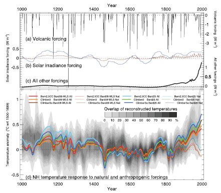
Figure 6.14. Simulated temperatures during the last 1 kyr with and without anthropogenic forcing, and also with weak or strong solar irradiance variations. Global mean radiative forcing (Wm–2)used to drive climate model simulations due to (a) volcanic activity, (b) strong (blue) and weak (brown) solar irradiance variations, and (c) all other forcings, including greenhouse gases and tropospheric sulphate aerosols (the thin flat line after 1765 indicates the fixed anthropogenic forcing used in the ‘Nat’ simulations). (d) Annual mean NH temperature (°C) simulated by three climate models under the forcings shown in (a) to (c), compared with the concentration of overlapping NH temperature reconstructions (shown by grey shading, modified from Figure 6.10c to account for the 1500 to 1899 reference period used here). ‘All’ (thick lines) used anthropogenic and natural forcings; ‘Nat’ (thin lines) used only natural forcings. All forcings and temperatures are expressed as anomalies from their 1500 to 1899 means; the temperatures were then smoothed with a Gaussian-weighted filter to remove fluctuations on time scales less than 30 years. Note the different vertical scale used for the volcanic forcing compared with the other forcings. The individual series are identified in Table 6.3 .
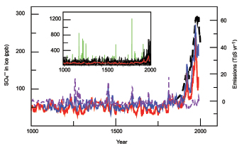
Figure 6.15. Sulphate (SO42–)concentrations in Greenland ( (Bigler et al., 2002, ) red line; Mieding, 2005 [NPR] , blue) and antarctic ( (Traufetter et al., 2004, ) dash, violet) ice cores during the last millennium. Also shown are the estimated anthropogenic sulphur (S) emissions for the NH ( (Stern, 2005; ) dashed black). The ice core data have been smoothed with a 10-year running median filter, thereby removing the peaks of major volcanic eruptions. The inset illustrates the influence of volcanic emissions over the last millennium and shows monthly sulphate data in ppm as measured (green), with identified volcanic spikes removed (black, most recent volcanic events were not assigned nor removed), and results from the 10-year filter (red) ( (Bigler et al., 2002 ) ). The records represent illustrative examples and can be influenced by local deposition events.
6.6.3.3 Industrial Era Sulphate Aerosols
Ice core data from Greenland and the mid-latitudes of the NH ( Schwikowski et al., 1999 [JoC] ;( Bigler et al., 2002 ) ) provide evidence of the rapid increase in sulphur dioxide emissions ( (Stern, 2005 ) ) and tropospheric sulphate aerosol loading, above the pre-industrial background, during the modern industrial era but they also show a very recent decline in these emissions( Figure 6.15 ). Data from ice cores show that sulphate aerosol deposition has not changed on Antarctica, remote from anthropogenic sulphur dioxide sources. The ice records are indicative of the regional-to-hemispheric scale atmospheric loading of sulphate aerosols that varies regionally as aerosols have a typical lifetime of only weeks in the troposphere. In recent years, sulphur dioxide emissions have decreased globally and in many regions of the NH ( (Stern, 2005; ) see Chapter2 ). In general, tropospheric sulphate aerosols exert a negative temperature forcing that will be less if sulphur dioxide emissions and the sulphate loading in the atmosphere continue to decrease.
6.6.3.4 Comparing Simulations of Northern Hemisphere Mean Temperatures with Palaeoclimatic Observations
Various simulations of NH (mean land and marine) surface temperatures produced by a range of climate models, and the forcings that were used to drive them, are shown in Figure 6.13 .Despite differences in the detail and implementation of the different forcing histories, there is generally good qualitative agreement between the simulations regarding the major features: warmth during much of the 12th through 14th centuries, with lower temperatures being sustained during the 17th, mid 15th and early 19th centuries, and the subsequent sharp rise to unprecedented levels of warmth at the end of the 20th century. The spread of this multi-model ensemble is constrained to be small during the 1500 to 1899 reference period (selected following Osborn et al., 2006 [Ambiguous] ), but the model spread also remains small back to 1000, with the exception of the ECHO-G simulation ( Von Storch et al., 2004 [JoC] ). The implications of the greater model spread in the rates of warming after 1840 will be clear only after determining the extent to which it can be attributed to differences in prescribed forcings and individual model sensitivities ( Goosse et al., 2005b [JoC, MoS, ARC] ). The ECHO-G simulation (dashed red line in Figure 6.13 d) is atypical compared to the ensemble as a whole, being notably warmer in the pre- 1300 and post- 1900 periods. Osborn et al. 2006 [Ambiguous] ) showed that these anomalies are likely the result of a large initial disequilibrium and the lack of anthropogenic tropospheric aerosols in that simulation (see Figure 6.13 c). One other simulation ( González-Rouco et al., 2006 [JoC, MoS, ARC] ) also exhibits greater early 20th-century warming in comparison to the other simulations but, similarly, does not include tropospheric aerosols among the forcings. All of these simulations, therefore, appear to be consistent with the reconstructions of past NH temperatures, for which the evidence (taken from Figure 6.10 c) is shown by the grey shading underlying the simulations in Figure 6.13 d.
It is important to note that many of the simulated temperature variations during the pre-industrial period shown in Figure 6.13 have been driven by assumed solar forcing, the magnitude of which is currently in doubt. Therefore, although the data and simulations appear consistent at this hemispheric scale, they are not a powerful test of the models because of the large uncertainty in both the reconstructed NH changes and the total radiative forcing. The influence of solar irradiance variability and anthropogenic forcings on simulated NH surface temperature is further illustrated in Figure 6.14 .A range of EMICs ( Petoukhov et al., 2000 [JoC, MoS, ARC] ; Plattner et al., 2001 [PoC, JoC, SRC] ; Montoya et al., 2005 [JoC, MoS] ) were forced with two different reconstructions of solar irradiance ( Bard et al., 2000 [JoC, SRC] ; Y.M. Wang et al., 2005 [JoC] ) to compare the influence of large versus small changes in the long-term strength of solar irradiance over the last 1 kyr( Figure 6.14 b). Radiative forcing related to explosive volcanism ( Crowley, 2000 [PoC, JoC] ), atmospheric CO2 and other anthropogenic agents ( Joos et al., 2001 [PoC, JoC, SRC] ) were identically prescribed within each model simulation. Additional simulations, in which anthropogenic forcings were not included, enable a comparison to be made between ‘natural’ versus ‘all’ (i.e., natural plus anthropogenic) forcings on the evolution of hemispheric temperatures before and during the 20th century.
The alternative solar irradiance histories used in the simulations differ in their low-frequency amplitudes by a factor of about three. The ‘high-amplitude’ case (strong solar irradiance forcing) corresponds roughly with the level of irradiance change assumed in many of the simulations shown in Figure 6.13 b, whereas the ‘low-amplitude’ case (weaker solar irradiance forcing) is representative of the more recent reconstructions of solar irradiance changes (as discussed in Section 6.6.3 ). The high-amplitude forcing history (‘Bard25’, Table 6.3 )is based on an ice core record of 10Be scaled to give an average reduction in solar irradiance of 0.25% during the Maunder Minimum, as compared to today ( Bard et al., 2000 [JoC, SRC] ). The low-amplitude history (‘Bard08-WLS’) is estimated using sunspot data and a model of the Sun’s closed magnetic flux for the period from 1610 to the present (Y.M. Wang et al., 2005 [JoC] ), with an earlier extension based on the Bard et al. 2000 [JoC, SRC] ) record scaled to a Maunder Minimum reduction of 0.08% compared to today. The low-frequency evolution of these two reconstructions is very similar( Figure 6.14 )even though they are based on completely independent sources of observational data (sunspots versus cosmogenic isotopes) and are produced differently (simple linear scaling versus modelled Sun’s magnetic flux) after 1610 .
Table 6.3 .Simulations with intermediate complexity climate models shown in Figure 6.14.
| Modelsa: | |
|---|---|
| Bern2.5CC | Plattner et al., 2001 |
| Climber2 | Petoukhov et al., 2000 |
| Climber3a | Montoya et al., 2005 |
| Forcings: | |
| Volcanic | Forcing from Crowley (2000) used in all runs |
| Solar | ‘Bard25’ runs used strong solar irradiance changes, based on 10Be record scaled to give a Maunder Minimum irradiance 0.25% lower than today, from Bard et al. (2000) |
| ‘Bard08-WLS’ runs used weak solar irradiance changes, using sunspot records and a model of the Sun’s magnetic flux for the period since 1610, from Y.M. Wang et al. (2005), and extended before this by the 10Be record scaled to give a Maunder Minimum irradiance 0.08% lower than today | |
| Anthropogenic | ‘All’ runs included anthropogenic forcings after 1765, from Joos et al. (2001) |
| ‘Nat’ runs did not include any anthropogenic forcings | |
The EMIC simulations shown in Figure 6.14 ,like those in Figure 6.13 d, fall within the range of proxy-based NH temperature reconstructions shown in Figure 6.10 cand are compatible with reconstructed and observed 20th-century warming only when anthropogenic forcings are incorporated. The standard deviation of multi-decadal variability in NH SAT is greater by 0.04°C to 0.07°C for the stronger solar forcing (Bard25, Table 6.3 )compared to the weaker solar forcing (Bard08-WLS). The uncertainty associated with the proxy-based temperature reconstructions and climate sensitivity of the models is too large to establish, based on these simulations, which of the two solar irradiance histories is the most likely. However, in the simulations that do not include anthropogenic forcing, NH temperatures reach a peak in the middle of the 20th century, and decrease afterwards, for both the strong and weak solar irradiance cases. This suggests that the contribution of natural forcing to observed 20th-century warming is small, and that solar and volcanic forcings are not responsible for the degree of warmth that occurred in the second half of the 20th century, consistent with the evidence of earlier work based on simple and more complex climate models ( Crowley and Lowery, 2000 [PoC, JoC] ; Bertrand et al., 2002b [JoC, SRC] ; Gerber et al., 2003 [JoC, MoS] ; Hegerl et al., 2006 [PoC, JoC, ARC] ; Tett et al., 2007 [JoC, MoS, ARC, 2007] ; see also Chapter9 ).
An overall conclusion can be drawn from the available instrumental and proxy evidence for the history of hemispheric average temperature change over the last 500 to 2,000 years, as well as the modelling studies exploring the possible roles of various causal factors: that is, greenhouse gases must be included among the forcings in order to simulate hemispheric mean temperatures that are compatible with the evidence of unusual warmth observed in the second half of the 20th century. It is very unlikely that this warming was merely a recovery from a pre-20th century cold period.
6.6.4 Consistency Between Temperature, Greenhouse Gas and Forcing Records; and Compatibility of Coupled Carbon Cycle-Climate Models with the Proxy Records
It is difficult to constrain the climate sensitivity from the proxy records of the last millennium (see Chapter9 ). As noted above, the evidence for hemispheric temperature change as interpreted from the different proxy records, and for atmospheric trace greenhouse gases, inferred solar forcing and reconstructed volcanic forcing, is to varying degrees uncertain. The available temperature reconstructions suggest that decadally averaged NH temperatures varied within 1°C or less during the two millennia preceding the 20th century( Figure 6.10 ), but the magnitude of the reconstructed low-frequency variations differs by up to about a factor of two for different reconstructions. The reconstructions of natural forcings (solar and volcanic) are uncertain for this period. If they produced substantial negative energy balances (reduced solar, increased volcanic activity), then low-to-medium estimates of climate sensitivity are compatible with the reconstructed temperature variations( Figure 6.10 ); however, if solar and volcanic forcing varied only weakly, then moderate-to-high climate sensitivity would be consistent with the temperature reconstructions, especially those showing larger cooling (see also Chapter9 ), assuming that the sensitivity of the climate system to solar irradiance changes and explosive volcanism is not different than the sensitivity to changes in greenhouse gases or other forcing agents.
The greenhouse gas record provides indirect evidence for a limited range of low-frequency hemispheric-scale climate variations over the last two millennia prior to the industrial period (AD 1– 1750 ). The greenhouse gas histories of CO2,CH4 andN2Oshow only small changes over this time period ( MacFarling Meure et al., 2006 [JoC] ; Figure 6.4 ), although there is evidence from the ice core record (Figures 6.3 and 6.7 ), as well as from models, that greenhouse gas concentrations react sensitively to climatic changes.
The sensitivity of atmospheric CO2 to climatic changes as simulated by coupled carbon cycle-climate models is broadly consistent with the ice core CO2 record and the amplitudes of the pre-industrial, decadal-scale NH temperature changes in the proxy-based reconstructions ( Joos and Prentice, 2004 [NPR, PoC, SRC] ). The CO2 climate sensitivity can be formally defined as the change in atmospheric CO2 relative to a nominal change in NH temperature in units of ppm per °C. Its strength depends on several factors, including the change in solubility of CO2 in seawater, and the responses of productivity and heterotrophic respiration on land to temperature and precipitation (see Section 7.3 ). The sensitivity was estimated for modest (NH temperature change less than about 1°C) temperature variations from simulations with the Bern Carbon Cycle-Climate model driven with solar and volcanic forcing over the last millennium ( Gerber et al., 2003 [JoC, MoS] ) and from simulations with the range of models participating in the Coupled Carbon Cycle-Climate Model Intercomparison Project (C4MIP) over the industrial period ( Friedlingstein et al., 2006 [JoC, MoS, ARC] ). The range of the CO2 climate sensitivity is 4 to 16 ppm per °C for the 10 models participating in theC4MIP intercomparison (evaluated as the difference in atmospheric CO2 for the 1990 decade between a simulation with, and without, climate change, divided by the increase in NH temperature from the 1860 decade to the 1990 decade). This is comparable to a range of 10 to 17 ppm per °C obtained for CO2 variations in the range of 6 to 10 ppm ( Etheridge et al., 1996 [JoC, ARC] ; Siegenthaler et al., 2005b [JoC] ) and the illustrative assumption that decadally averaged NH temperature varied within 0.6°C.
6.6.5 Regional Variability in Quantities Other than Temperature
6.6.5.1 Changes in the El Niño-Southern Oscillation System
Considerable interest in the ENSO system has encouraged numerous attempts at its palaeoclimatic reconstruction. These include a boreal winter (December–February) reconstruction of the Southern Oscillation Index (SOI) based on ENSO-sensitive tree ring indicators ( Stahle et al., 1998 [JoC] ), two multi-proxy reconstructions of annual and October to March Niño 3 index (average SST anomalies over 5°N to 5°S, 150°W to 90°W; Mann et al., 2005a [PoC, JoC, MoS, ARC] ,b), and a tropical coral-based Niño 3.4 SST reconstruction ( Evans et al., 2002 [JoC] ). Fossil coral records from Palmyra Island in the tropical Pacific also provide 30- to 150-year windows of ENSO variability within the last 1.1 kyr ( Cobb et al., 2003 [JoC] ). Finally, a new 600-year reconstruction of December to February Niño-3 SST has recently been developed ( D’Arrigo et al., 2005 [JoC] ), which is considerably longer than previous series. Although not totally independent (i.e., the reconstructions share a number of common predictors), these palaeorecords display significant common variance (typically more than 30% during their respective cross-validation periods), suggesting a relatively consistent history of El Niño in past centuries ( Jones and Mann, 2004 [PoC, JoC, ARC] ). In most coral records from the western Pacific and the Indian Ocean, late 20th-century warmth is unprecedented over the past 100 to 300 years ( Bradley et al., 2003b [NPR, PoC, MoS, SRC] ). However, reliable and consistent interpretation of geochemical records from corals is still problematic ( (Lough, 2004 ) ). Reconstructions of extratropical temperatures and atmospheric circulation features (e.g., the North Pacific Index) correlate significantly with tropical estimates, supporting evidence for tropical/high-latitude Pacific links during the past three to four centuries ( Evans et al., 2002 [JoC] ; Linsley et al., 2004 [JoC] ; D’Arrigo et al., 2006 [JoC] ).
The El Niño-Southern Oscillation may have responded to radiative forcing induced by solar and volcanic variations over the past millennium ( Adams et al., 2003 [PoC, JoC, MoS, ARC] ; Mann et al., 2005a [PoC, JoC, MoS, ARC] ). Model simulations support a statistically significant response of ENSO to radiative changes such that during higher radiative inputs, la Niña-like conditions result from an intensified zonal SST gradient that drives stronger trade winds, and vice versa ( Mann et al., 2005a [PoC, JoC, MoS, ARC] ). Comparing data and model results over the past millennium suggests that warmer background conditions are associated with higher variability ( Cane, 2005 [MoS] ). Numerical experiments suggest that the dynamics of ENSO may have played an important role in the climatic response to past changes in radiative forcing ( Mann et al., 2005b [PoC, JoC, ARC] ). Indeed, the low-frequency changes in both amplitude of variability and mean state indicated by ENSO reconstructions from Palmyra corals ( Cobb et al., 2003 [JoC] ) were found to correspond well with the model responses to changes in tropical volcanic radiative forcing over the past 1 kyr, with solar forcing playing a secondary role.
Proxy records suggest that ENSO’s global climate imprint evolves over time, complicating predictions. Comparisons of ENSO and drought indices clearly show changes in the linkage between ENSO and moisture balance in the USA over the past 150 years. Significant ENSO-drought correlations occur consistently in the southwest USA, but the strength of moisture penetration into the continent varies substantially over time ( Cole and Cook, 1998 [PoC, JoC, SRC] ; Cook et al., 2000 [PoC, JoC, SRC] ). Comparing reconstructed Niño 3 SST with global temperature patterns suggests that some features are robust through time, such as the warming in the eastern tropical Pacific and western coasts of North and South America, whereas teleconnections into North America, the Atlantic and Eurasia are variable ( Mann et al., 2000 [NPR, PoC] ). The spatial correlation pattern for the period 1801 to 1850 provides striking evidence of non-stationarity in ENSO teleconnections, showing a distinct absence of the typical pattern of tropical Pacific warming ( Mann et al., 2000 [NPR, PoC] ).
6.6.5.2 The Record of Past Atlantic Variability
Climate variations over the North Atlantic are related to changes in the NAO ( Hurrell, 1995 [JoC, ARC] ) and the Atlantic Multidecadal Oscillation ( Delworth and Mann, 2000 [PoC, JoC, MoS, ARC] ; Sutton and Hodson, 2005 [JoC, MoS] ). From 1980 to 1995, the NAO tended to remain in one extreme phase and accounted for a substantial part of the winter warming over Europe and northern Eurasia. The North Atlantic region has a unique combination of long instrumental observations, many documentary records and multiple sources of proxy records. However, it remains difficult to document past variations in the dominant modes of climate variability in the region, including the NAO, due to problems of establishing proxies for atmospheric pressure, as well as the lack of stationarity in the NAO frequency and in storm tracks. Several reconstructions of NAO have been proposed ( Cook et al., 2002b [PoC, JoC, SRC] ; Cullen et al., 2002 [JoC] ; Luterbacher et al., 2002 [JoC, ARC] ). Although the reconstructions differ in many aspects, there is a general tendency for more negative NAO indices during the 17th and 18th centuries than in the 20th century, thus indicating that the colder mean climate was characterised by a more zonal atmospheric pattern than in the 20th century. The coldest reconstructed European winter in 1708 / 1709, and the strong warming trend between 1684 and 1738 (+0.32°C per decade), have been related to a negative NAO index and the NAO response to increasing radiative forcing, respectively ( Luterbacher et al., 2004 [JoC, ARC] ). Some spatially resolved simulations employing GCMs indicate that solar and volcanic forcings lead to continental warming associated with a shift towards a high NAO index ( Shindell et al., 2001 [JoC, MoS] , 2003, 2004; Stendel et al., 2006 [JoC, MoS, ARC] ). Increased solar irradiance at the end of the 17th century and through the first half of the 18th century might have induced such a shift towards a high NAO index ( Shindell et al., 2001 [JoC, MoS] ; Luterbacher et al., 2004 [JoC, ARC] ; Xoplanki et al., 2005 ).
It is well known that the NAO exerts a dominant influence on winter temperature and precipitation over Europe, but the strength of the relationship can change over time and region ( Jones et al., 2003 [Ambiguous] ). The strong trend towards a more positive NAO index in the early part of the 18th century in the Luterbacher et al. 2002 [JoC, ARC] ) NAO reconstruction appears connected with positive winter precipitation anomalies over northwest Europe and marked expansions of maritime glaciers in a manner similar to the effect of positive winter precipitation anomalies over recent decades for the same glaciers ( Nesje and Dahl, 2003 [JoC] ; Pauling et al., 2006 [JoC, ARC] ).
6.6.5.3 Asian Monsoon Variability
Fifteen severe (three years or longer) droughts have occurred in a region of China dominated by the East Asian Monsoon over the last 1 kyr ( (Zhang, 2005 ) ). These palaeodroughts were generally more severe than droughts in the same region within the last 50 years. In contrast, the South Asian (Indian) monsoon, in the drier areas of its influence, has recently reversed its millennia-long orbitally driven low-frequency trend towards less rainfall. This recent reversal in monsoon rainfall also appears to coincide with a synchronous increase in inferred monsoon winds over the western Arabian Sea ( Anderson et al., 2002 [PoC, JoC, SRC] ), a change that could be related to increased summer heating over and around the Tibetan Plateau ( Braüning and Mantwill, 2004 [JoC] ;( Morrill et al., 2006 ) ).
Lake sediment and historical documentary evidence indicate that northern Africa and the Sahel region have for a long time experienced substantial droughts lasting from decades to centuries ( Kadomura, 1992 [NPR] ;( Verschuren, 2001; ) ( Russell et al., 2003; ) ( Stager et al., 2003; ) Nguetsop et al., 2004 [JoC] ;( Brooks et al., 2005; ) ( Stager et al., 2005 ) ). Although there have been attempts to link these dry periods to solar variations, the evidence is not conclusive ( (Stager et al., 2005 ) ), particularly given that the relationship between hypothesised solar proxies and variation in total solar irradiance remains unclear (see Section 6.6.3 ). The palaeoclimate record indicates that persistent droughts have been a common feature of climate in northern and eastern Africa. However, it has not been demonstrated that these droughts can be simulated with coupled ocean-atmosphere models.
6.6.5.5 The Record of Hydrologic Variability and Change in the Americas
Multiple proxies, including tree rings, sediments, historical documents and lake sediment records make it clear that the past 2 kyr included periods with more frequent, longer and/or geographically more extensive droughts in North America than during the 20th century ( Stahle and Cleaveland, 1992 [JoC] ; Stahle et al., 1998 [JoC] ; Woodhouse and Overpeck, 1998 [PoC, JoC, SRC] ; Forman et al., 2001 [JoC] ; Cook et al., 2004b [PoC, JoC, SRC] ; Hodell et al., 2005 [JoC] ; MacDonald and Case, 2005 [JoC] ). Past droughts, including decadal-length ‘megadroughts’ ( Woodhouse and Overpeck, 1998 [PoC, JoC, SRC] ), are most likely due to extended periods of anomalous SST ( Hoerling and Kumar, 2003 [JoC] ; Schubert et al., 2004 [JoC] ; MacDonald and Case, 2005 [JoC] ; Seager et al., 2005 [JoC, MoS] ), but remain difficult to simulate with coupled ocean-atmosphere models. Thus, the palaeoclimatic record suggests that multi-year, decadal and even centennial-scale drier periods are likely to remain a feature of future North American climate, particularly in the area west of the Mississippi River.
There is some evidence that North American drought was more regionally extensive, severe and frequent during past intervals that were characterised by warmer than average NH summer temperatures (e.g., during medieval times and the mid-Holocene; Forman et al., 2001 [JoC] ; Cook et al., 2004b [PoC, JoC, SRC] ). There is evidence that changes in the North American hydrologic regime can occur abruptly relative to the rate of change in climate forcing and duration of the subsequent climate regime. Abrupt shifts in drought frequency and duration have been found in palaeohydrologic records from western North America ( Cumming et al., 2002 [JoC] ; Laird et al., 2003 [JoC] ; Cook et al., 2004b [PoC, JoC, SRC] ). Similarly, the upper Mississippi River Basin and elsewhere have seen abrupt shifts in the frequency and size of the largest flood events ( Knox, 2000 [JoC] ). Recent investigations of past large-hurricane activity in the southeast USA suggest that changes in the regional frequency of large hurricanes can shift abruptly in response to more gradual forcing ( Liu, 2004 [NPR, MoS] ). Although the palaeoclimatic record indicates that hydrologic shifts in drought, floods and tropical storms have occurred abruptly (i.e., within years), this past abrupt change has not been simulated with coupled atmosphere ocean models. Decadal variability of Central Chilean precipitation was greater before the 20th century, with more intense and prolonged dry episodes in the past. Tree-ring based precipitation reconstructions for the past eight centuries reveal multi-year drought episodes in the 14th and 16th to 18th centuries that exceed the estimates of decadal drought during the 20th century (LeQuesne et al., 2006 ).
6.7 Concluding Remarks on Key Uncertainties
Each palaeoclimatic time scale covered in this chapter contributes to the understanding of how the climate system varies naturally and also responds to changes in climate forcing. The existing body of knowledge is sufficient to support the assertions of this chapter. At the same time, key uncertainties remain, and greater confidence would result if these uncertainties were reduced.
Even though a great deal is known about glacial-interglacial variations in climate and greenhouse gases, a comprehensive mechanistic explanation of these variations remains to be articulated. Similarly, the mechanisms of abrupt climate change (for example, in ocean circulation and drought frequency) are not well enough understood, nor are the key climate thresholds that, when crossed, could trigger an acceleration in sea level rise or regional climate change. Furthermore, the ability of climate models to simulate realistic abrupt change in ocean circulation, drought frequency, flood frequency, ENSO behaviour and monsoon strength is uncertain. Neither the rates nor the processes by which ice sheets grew and disintegrated in the past are known well enough.
Knowledge of climate variability over the last 1 to 2 kyr in the SH and tropics is severely limited by the lack of palaeoclimatic records. In the NH, the situation is better, but there are important limitations due to a lack of tropical records and ocean records. Differing amplitudes and variability observed in available millennial-length NH temperature reconstructions, and the extent to which these differences relate to choice of proxy data and statistical calibration methods, need to be reconciled. Similarly, the understanding of how climatic extremes (i.e., in temperature and hydro-climatic variables) varied in the past is incomplete. Lastly, this assessment would be improved with extensive networks of proxy data that run right up to the present day. This would help measure how the proxies responded to the rapid global warming observed in the last 20 years, and it would also improve the ability to investigate the extent to which other, non-temperature, environmental changes may have biased the climate response of proxies in recent decades.
References
Adams, J.B., M.E. Mann, and C.M. Ammann, 2003: Proxy evidence for an El Niño-like response to volcanic forcing. Nature, 426(6964), 274–278. [PoC, JoC, MoS, ARC]
Adkins, J.F., K. McIntyre, and D.P. Schrag, 2002: The salinity, temperature, and δ18Oof the glacial deep ocean. Science, 298,1769–1773. [JoC]
Alley, R.B., and P.U. Clark, 1999: The deglaciation of the northern hemisphere: A global perspective. Annu. Rev. Earth Planet. Sci., 27,149–182. [ARC]
Alley, R.B., and A.M. Agustsdottir, 2005: The 8k event: cause and consequences of a major Holocene abrupt climate change. Quat. Sci. Rev., 24,1123–1149. [JoC, ARC]
Alley, R.B., S. Anandakrishnan, and P. Jung, 2001: Stochastic resonance in the North Atlantic. Paleoceanography, 16,190–198. [JoC, ARC]
Alley, R.B., et al., 1997: Holocene climatic instability: A large, widespread event 8200 years ago. Geology, 25,483–486. [ARC]
Alley, R.B., et al., 2003: Abrupt climate change. Science, 299(5615), 2005–2010. [JoC, ARC]
Alverson, K.D., R.S. Bradley, and T.F. Pedersen (eds.), 2003: Paleoclimate, Global Change and the Future. International Geosphere Biosphere Programme Book Series, Springer-Verlag, Berlin, 221 pp. [NPR, PoC, MoS]
Ammann, C.M., G.A. Meehl, W.M. Washington, and C.S. Zender, 2003: A monthly and latitudinally varying volcanic forcing dataset in simulations of 20th century climate. Geophys. Res. Lett., 30(12), 1657, doi:10.1029/2003GL016875. [PoC, JoC, MoS, ARC]
Andersen, C., N. Koç, A. Jennings, and J.T. Andrews, 2004: Non uniform response of the major surface currents in the Nordic Seas to insolation forcing: implications for the Holocene climate variability. Paleoceanography, 19,1–16. [JoC, MoS]
Anderson, D.M., J.T. Overpeck, and A.K. Gupta, 2002: Increase in the Asian southwest monsoon during the past four centuries. Science, 297(5581), 596–599. [PoC, JoC, SRC]
Archer, D., and A. Ganopolski, 2005: A movable trigger: Fossil fuel CO2 and the onset of the next glaciation. Geochem. Geophys. Geosystems, 6,Q05003. [ARC]
Archer, D.A., A. Winguth, D. Lea, and N. Mahowald, 2000: What caused the glacial/interglacial atmospheric pCO2 cycles? Rev. Geophys., 12,159–189. [JoC, ARC]
Ariztegui, D., et al., 2000: Paleoclimate and the formation of sapropel S1: inferences from Late Quaternary lacustrine and marine sequences in the central Mediterranean region. Palaeogeogr. Palaeoclimatol. Palaeoecol., 158,215–240. Clean
Bakke, J., S.O. Dahl, and A. Nesje, 2005a: Late glacial and early Holocene palaeoclimatic reconstruction based on glacier fluctuations and equilibrium-line altitudes at northern Folgefonna, Hardanger, western Norway. J. Quat. Sci., 20(2), 179–198. Clean
Bakke, J., et al., 2005b: Glacier fluctuations, equilibrium-line altitudes and palaeoclimate in Lyngen, northern Norway, during the Late glacial and Holocene. The Holocene, 15(4), 518–540. [JoC]
Baliunas, S., and R. Jastrow, 1990: Evidence for long-term brightness changes of solar-type stars. Nature, 348,520–522. [JoC]
Ballantyne, A.P., et al., 2005: Meta-analysis of tropical surface temperatures during the Last Glacial Maximum. Geophys. Res. Lett., 32,L05712, doi:10.1029/2004GL021217. [JoC]
Bao, Y., A. Brauning, and S. Yafeng, 2003: Late Holocene temperature fluctuations on the Tibetan Plateau. Quat. Sci. Rev., 22(21), 2335–2344. [JoC]
Barber, D.C., et al., 1999: Forcing of the cold event of 8,200 years ago by catastrophic drainage of Laurentide lakes. Nature, 400,344–347. [JoC, MoS]
Bard, E., G. Raisbeck, F. Yiou, and J. Jouzel, 2000: Solar irradiance during the last millennium based on cosmogenic nucleides. Tellus, 52B,985–992. [JoC, SRC]
Barrows, T.T., and S. Juggins, 2005: Sea-surface temperatures around the Australian margin and Indian Ocean during the Last Glacial Maximum. Quat. Sci. Rev., 24,1017–1047. [JoC]
Bartlett, M.G., D.S. Chapman, and R.N. Harris, 2004: Snow and the ground temperature record of climate change. J. Geophys Res., 109,F04008, doi:10.1029/2004JF000224. [JoC]
Battle, M., et al., 1996: Atmospheric gas concentrations over the past century measured in air from firn at the South Pole. Nature, 383(6597), 231–235. [JoC]
Bauer, E., A. Ganopolski, and M. Montoya, 2004: Simulation of the cold climate event 8200 years ago by meltwater outburst from Lake Agassiz. Paleoceanography, 19,PA3014, doi:10.1029/2004PA001030. [JoC, MoS, SRC]
Bauer, E., M. Claussen, V. Brovkin, and A. Huenerbein, 2003: Assessing climate forcings of the Earth system for the past millennium. Geophys. Res. Lett., 30(6), 1276, doi:10.1029/2002GL016639. [JoC, MoS, SRC]
Beer, J., S. Tobias, and N. Weiss, 1998: An active sun throughout the Maunder Minimum. Sol. Phys., 181(1), 237–249. Clean
Beerling, D.J., 1999: New estimates of carbon transfer to terrestrial ecosystems between the last glacial maximum and the Holocene. Terra Nova, 11(4), 162–167. [MoS]
Beltrami, H., 2002: Paleoclimate: Earth’s long-term memory. Science, 297(5579), 206–207. [JoC]
Beltrami, H., and E. Bourlon, 2004: Ground warming patterns in the Northern Hemisphere during the last five centuries. Earth Planet. Sci. Lett., 227(3–4), 169–177. Clean
Berger, A., 1977: Long-term variations of earth’s orbital elements. Celestial Mechanics, 15(1), 53–74. [ARC]
Berger, A., 1978: Long-term variation of caloric solar radiation resulting from the earth’s orbital elements. Quat. Res., 9,139–167. [ARC]
Berger, A.L., and M.F. Loutre, 1991: Insolation values for the climate of the last 10 million years. Quat. Sci. Rev., 10,297–317. [JoC, SRC]
Berger, A.L., and M.F. Loutre, 2002: An exceptionally long interglacial ahead? Science, 297,1287–1288. [JoC, SRC]
Berger, A.L., and M.F. Loutre, 2003: Climate 400,000 years ago, a key to the future? In: Earth’s Climate and Orbital Eccentricity [Droxler, A.W., R.Z. Poore, and L.H. Burckle (eds.)]. American Geophysical Union, Washington, DC, pp. 17–26. [NPR, MoS, SRC]
Berggren, W.A., D.V. Kent, C.C.I. Swisher, and M.P. Aubry, 1995: Geochronology, Time Scales and Global Stratigraphic Correlation [W.A. Berggren (ed)]. Special Publication No. 54, Society for Sedimentary Geology, Tulsa, OK, 386 pp. [NPR]
Berner, R.A., and Z. Kothavala, 2001: GEOCARB III: A revised model of atmospheric CO2 over phanerozoic time. Am. J. Sci., 301(2), 182–204. [MoS]
Bertrand, C., M.F. Loutre, and A. Berger, 2002a: High frequency variations of the Earth’s orbital parameters and climate change. Geophys. Res. Lett., 29,doi:10.1029/2002GL015622. [NPR, JoC, SRC]
Bertrand, C., M.F. Loutre, M. Crucifix, and A. Berger, 2002b: Climate of the last millennium: a sensitivity study. Tellus, 54A(3), 221–244. [JoC, SRC]
Bianchi, G., and I.N. McCave, 1999: Holocene periodicity in north Atlantic climate and deep ocean flow south of Iceland. Nature, 397,515–518. [JoC]
Bigelow, N., et al., 2003: Climate change and Arctic ecosystems: 1. Vegetation changes north of 55 degrees N between the last glacial maximum, mid-Holocene, and present. J. Geophys. Res., 108,doi:10.1029/2002JD002558. [JoC]
Bigler, M., et al., 2002: Sulphate record from a northeast Greenland ice core over the last 1200 years based on continuous flow analysis. Ann. Glaciol., 35,250–256. Clean
Billups, K., J.E.T. Channell, and J. Zachos, 2002: Late Oligocene to early Miocene geochronology and paleoceanography from the subantarctic South Atlantic. Paleoceanography, 17(1), 1004, doi:10.1029/2000PA000568. [JoC, SRC]
Bird, M.I., J. Lloyd, and G.D. Farquhar, 1994: Terrestrial carbon storage at the LGM. Nature, 371(6498), 566–566. [JoC]
Birks, H.H., and B. Ammann, 2000: Two terrestrial records of rapid climatic change during the glacial-Holocene transition (14,000-9,000 calendar years B.P.) from Europe. Proc. Natl. Acad. Sci. U.S.A., 97,1390–1394. [JoC]
Bjerknes, J., 1969: Atmospheric teleconnections from equatorial pacific. Mon. Weather Rev., 97(3), 163–172 [JoC]
Blunier, T., and E.J. Brook, 2001: Timing of millennial-scale climate change in Antarctica and Greenland during the last glacial period. Science, 291,109–112. [JoC]
Blunier, T., et al., 1993: Atmospheric methane record from a Greenland ice core over the last 1000 years. Geophys. Res. Lett., 20(20), 2219–2222. [JoC]
Blunier, T., et al., 1995: Variations in atmospheric methane concentration during the Holocene epoch. Nature, 374(6517), 46–49. [JoC]
Blunier, T., et al., 1998: Asynchrony of Antarctic and Greenland climate change during the last glacial period. Nature, 394,739–743. [JoC]
Bohaty, S.M., and J.C. Zachos, 2003: Significant Southern Ocean warming event in the late middle Eocene. Geology, 31(11), 1017–1020. [SRC]
Bond, G., et al., 1993: Correlations between climate records from North Atlantic sediments and Greenland ice. Nature, 365,143–147. [JoC]
Bond, G., et al., 1997: A pervasive millennial-scale cycle in the North Atlantic Holocene and glacial climates. Science, 278,1257–1266. [JoC]
Bond, G., et al., 2001: Persistent solar influence on North Atlantic climate during the Holocene. Science, 294,2130–2136. [JoC]
Bond, W.J., G.F. Midgley, and F.I. Woodward, 2003: The importance of low atmospheric CO2 and fire in promoting the spread of grasslands and savannas. Global Change Biol., 9(7), 973–982. Clean
Booth, R.K., et al., 2005: A severe centennial-scale drought in mid-continental North America 4200 years ago and apparent global linkages. The Holocene, 15,321–328. [JoC]
Bopp, L., K.E. Kohlfeld, C. Le Quéré, and O.O. Aumont, 2002: Dust impact on marine biota and atmospheric CO2 in glacial periods. Geochim. Cosmochim. Acta, 66(15A), A91, Suppl. 1, Aug. 2002. [ARC]
Bowen, G.J., et al., 2002: Mammalian dispersal at the Paleocene/Eocene boundary. Science, 295(5562), 2062–2065. [JoC]
Bowen, G.J., et al., 2004: A humid climate state during the Palaeocene/Eocene thermal maximum. Nature, 432(7016), 495–499. [JoC]
Braconnot, P., O. Marti, S. Joussaume, and Y. Leclaninche, 2000: Ocean feedbacks in response to 6 kyr insolation. J. Clim., 13,1537–1553. [JoC, ARC]
Braconnot, P., et al., 2002: How the simulated change in monsoon at 6 ka BP is related to the simulation of the modern climate: results from the Paleoclimate Modeling Intercomparison Project. Clim. Dyn., 19(2), 107–121. [JoC, MoS, ARC]
Braconnot, P., et al., 2004: Evaluation of PMIP coupled ocean-atmosphere simulations of the Mid-Holocene. In: Past Climate Variability through Europe and Africa,Vol. 6 [Battarbee, R.W., F. Gasse, and C.E. Stickley (eds)], Springer, Dordrecht, The Netherlands, 515–534. [NPR, ARC]
Bradley, R.S., 1999: Climatic variability in sixteenth-century Europe and its social dimension - Preface. Clim. Change, 43(1), 1–2. [PoC, JoC]
Bradley, R.S., M.K. Hughes, and H.F. Diaz, 2003a: Climate in Medieval time. Science, 302(5644), 404–405. [PoC, JoC]
Bradley, R.S., K.R. Briffa, J. Cole, and T.J. Osborn, 2003b: The climate of the last millennium. In: Paleoclimate, Global Change and the Future [Alverson, K.D., R.S. Bradley, and T.F. Pedersen (eds.)]. Springer, Berlin, pp. 105–141. [NPR, PoC, MoS, SRC]
Bralower, T.J., 2002: Evidence of surface water oligotrophy during the Paleocene-Eocene thermal maximum: Nannofossil assemblage data from Ocean Drilling Program Site 690, Maud Rise, Weddell Sea. Paleoceanography, 17(2), 1023, doi:10.1029/2001PA000662. [JoC]
Bräuning, A., and B. Mantwill, 2004: Summer temperature and summer monsoon history on the Tibetan plateau during the last 400 years recorded by tree rings. Geophys. Res. Lett., 31(24), L24205, doi:10.1029/2004GL020793. [JoC]
Briffa, K.R., 2000: Annual climate variability in the Holocene: interpreting the message of ancient trees. Quat. Sci. Rev., 19(1–5), 87–105. [PoC, JoC, SRC]
Briffa, K.R., and T.J. Osborn, 1999: Perspectives: Climate warming - Seeing the wood from the trees. Science, 284(5416), 926–927. [PoC, JoC, SRC]
Briffa, K.R., and T.J. Osborn, 2002: Paleoclimate - Blowing hot and cold. Science, 295(5563), 2227–2228. [PoC, JoC, SRC]
Briffa, K.R., T.J. Osborn, and F.H. Schweingruber, 2004: Large-scale temperature inferences from tree rings: a review. Global Planet. Change, 40(1–2), 11–26. [PoC, JoC, SRC]
Briffa, K.R., et al., 2001: Low-frequency temperature variations from a northern tree ring density network. J. Geophys. Res., 106(D3), 2929–2941. [PoC, JoC, SRC]
Brigham-Grette, J., and D.M. Hopkins, 1995: Emergent marine record and paleoclimate of the last interglaciation along the northwest Alaskan coast. Quat. Res., 43,159–173. Clean
Broecker, W.S., and G.M. Henderson, 1998: The sequence of events surrounding Termination II and their implications for the cause of glacial-interglacial CO2 changes. Paleoceanography, 13,352–364. [JoC]
Broecker, W.S., and E. Clark, 2003: Holocene atmospheric CO2 increase as viewed from the seafloor. Global Biogeochem. Cycles, 17(2), doi:10.1029/2002GB001985. [JoC]
Brook, E.J., et al., 2000: On the origin and timing of rapid changes in atmospheric methane during the last glacial period. Global Biogeochem. Cycles, 14(2), 559–572. [JoC]
Brooks, C.E.P., 1922: The Evolution of Climate.[Preface by Simpson, G.C.] Benn Brothers, London, 173 pp. [NPR]
Brooks, K., et al., 2005: Late-Quaternary lowstands of Lake Bosumtwi, Ghana: evidence from high-resolution seismic-reflection and sediment-core data. Palaeogeogr. Palaeoclimatol. Palaeoecol., 216(3–4), 235–249. Clean
Brovkin, V., et al., 2002: Carbon cycle, vegetation and climatic dynamics in the Holocene: Experiments with the CLIMBER-2 model. Global Biogeochem. Cycles, 16,1139, doi:10.1029/2001GB001662. [JoC, MoS, ARC]
Burger, G., and U. Cubasch, 2005: Are multiproxy climate reconstructions robust? Geophys. Res. Lett., 32(23), doi:10.1029/2005GL024155. [JoC, ARC]
Caillon, N., et al., 2003: Timing of atmospheric CO2 and Antarctic temperature changes across Termination III. Science, 299,1728–1731. [JoC]
Calov, R., A. Ganopolski, V. Petoukhov, and M. Claussen, 2002: Large-scale instabilities of the Laurentide ice sheet simulated in a fully coupled climate-system model. Geophys. Res. Lett., 29,2216, doi:10.1029/2002GL016078. [JoC, MoS, ARC]
Calov, R., et al., 2005: Transient simulation of the last glacial inception. Part II: Sensitivity and feedback analysis. Clim. Dyn., 24,563–576. [JoC, MoS]
Cane, M.A., 2005: The evolution of El Niño, past and future. Earth Planet. Sci. Lett., 230(3–4), 227–240. [MoS]
CAPE Last Interglacial Project Members, 2006: Last Interglacial Arctic warmth confirms polar amplification of climate change. Quat. Sci. Rev., 25(13–14), 1383–1400. [JoC]
Castellano, E., et al., 2005: Holocene volcanic history as recorded in the sulfate stratigraphy of the European Project for Ice Coring in Antarctica Dome C (EDC96) ice core. J. Geophys. Res., 110,D06114, doi:10.1029/2004JD005259. [JoC]
Cerling, T.E., 1991: Carbon dioxide in the atmosphere: Evidence from Cenozoic and Mesozoic paleosols. Am. J. Sci., 291,377–400. Clean
Chandler, M.A., D. Rind, and R.S. Thompson, 1994: Joint investigations of the middle Pliocene climate II: GISS GCM Northern Hemisphere results. Global Planet. Change, 9,197–219. [JoC, SRC]
Chapman, D.S., M.G. Bartlett, and R.N. Harris, 2004: Comment on “Ground vs. surface air temperature trends: Implications for borehole surface temperature reconstructions” by M. E. Mann and G. Schmidt. Geophys. Res. Lett., 31(7), L07205, doi:10.1029/2003GL019054. [JoC]
Chappellaz, J.A., I.Y. Fung, and A.M. Thompson, 1993: The atmospheric CH4 increase since the last glacial maximum. Tellus, B45(3), 228–241. [JoC, ARC]
Chappellaz, J., et al., 1997: Changes in the atmospheric CH4 gradient between Greenland and Antarctica during the Holocene. J. Geophys. Res., 102(D13), 15987–15997. [JoC]
Charles, C.D., D.E. Hunter, and R.G. Fairbanks, 1997: Interaction between the ENSO and the Asian monsoon in a coral record of tropical climate. Science, 277(5328), 925–928. [JoC]
Church, J.A., et al., 2001: Changes in sea level. In: Climate Change 2001: The Scientific Basis. Contribution of Working Group I to the Third Assessment Report of the Intergovernmental Panel on Climate Change [Houghton, J.T. et al. (eds.)]. Cambridge University Press, Cambridge, United Kingdom and New York, NY, USA, pp. 639–693. [NPR, ARC]
Claquin, T., et al., 2003: Radiative forcing of climate by ice-age atmospheric dust. Clim. Dyn., 20,193–202. [JoC, MoS]
Clark, P.U., N.G. Pisias, T.F. Stocker, and A.J. Weaver, 2002: The role of the thermohaline circulation in abrupt climate change. Nature, 415,863–869. [JoC, ARC]
Clarke, G.K.C., D.W. Leverington, J.T. Teller, and A.S. Dyke, 2004: Paleohydraulics of the last outburst flood from glacial Lake Agassiz and the 8200 BP cold event. Quat. Sci. Rev., 23,389–407. [JoC, ARC]
Claussen, M., and Gayler, V., 1997: The greening of Sahara during the mid-Holocene: results of an interactive atmosphere-biome model. Global Ecol. Biogeogr. Lett., 6,369–377. [MoS, ARC]
Claussen, M., et al., 1999: Simulation of an abrupt change in Saharan vegetation in the mid-Holocene. Geophys. Res. Lett., 26(14), 2037–2040. [JoC, MoS, ARC]
Claussen, M., et al., 2002: Earth system models of intermediate complexity: closing the gap in the spectrum of climate system models. Clim. Dyn., 18(7), 579–586. [JoC, MoS, ARC]
Clement, A.C., and M.A. Cane, 1999: A role for the tropical Pacific coupled ocean-atmosphere system on Milankovitch and millennial timescales. Part I: A modeling study of tropical Pacific variability. In: Mechanisms of Global Climate Change at Millennial Time Scales [Clark, P.U., R.S. Webb, and L.D. Keigwin (eds.)]. American Geophysical Union, Washington, DC, pp. 363–371. [NPR, MoS, ARC]
Clement, A.C., R. Seager, and M.A. Cane, 2000: Suppression of El Niño during the mid-Holocene by changes in the earth’s orbit. Paleoceanography, 15(6), 731–737. [JoC, ARC]
Clement, A.C., M.A. Cane, and R. Seager, 2001: An orbitally driven tropical source for abrupt climate change. J. Clim., 14(11), 2369–2375. [ARC]
Clement, A.C., R. Seager, M.A. Cane, and S.E. Zebiak, 1996: An ocean dynamical thermostat. J. Clim., 9(9), 2190–2196. [JoC, ARC]
Cobb, K.M., C.D. Charles, H. Cheng, and R.L. Edwards, 2003: El Niño/Southern Oscillation and tropical Pacific climate during the last millennium. Nature, 424(6946), 271–276. [JoC]
Coe, M.T., and S.P. Harrison 2002: The water balance of northern Africa during the mid-Holocene: an evaluation of the 6 ka BPPMIP simulations. Clim. Dyn., 19(2), 155–166. [JoC, MoS]
Cole, J., 2003: Global change - Dishing the dirt on coral reefs. Nature, 421(6924), 705–706. [JoC, SRC]
Cole, J.E., and E.R. Cook, 1998: The changing relationship between ENSO variability and moisture balance in the continental United States. Geophys. Res. Lett., 25(24), 4529–4532. [PoC, JoC, SRC]
Cole, J.E., R.B. Dunbar, T.R. McClanahan, and N.A. Muthiga, 2000: Tropical Pacific forcing of decadal SST variability in the western Indian Ocean over the past two centuries. Science, 287(5453), 617–619. [JoC, MoS, SRC]
Cook, E.R., J.G. Palmer, and R.D. D’Arrigo, 2002a: Evidence for a ‘Medieval Warm Period’ in a 1,100 year tree-ring reconstruction of past austral summer temperatures in New Zealand. Geophys. Res. Lett., 29(14), 1667, doi:10.1029/2001GL014580. [PoC, JoC, SRC]
Cook, E.R., R.D. D’Arrigo, and M.E. Mann, 2002b: A well-verified, multiproxy reconstruction of the winter North Atlantic Oscillation index since AD 1400. J. Clim., 15(13), 1754–1764. [PoC, JoC, SRC]
Cook, E.R., J. Esper, and R.D. D’Arrigo, 2004a: Extra-tropical Northern Hemisphere land temperature variability over the past 1000 years. Quat. Sci. Rev., 23(20–22), 2063–2074. [PoC, JoC, SRC]
Cook, E.R., B.M. Buckley, R.D. D’Arrigo, and M.J. Peterson, 2000: Warm-season temperatures since 1600 BC reconstructed from Tasmanian tree rings and their relationship to large-scale sea surface temperature anomalies. Clim. Dyn., 16(2–3), 79–91. [PoC, JoC, SRC]
Cook, E.R., et al., 2004b: Long-term aridity changes in the western United States. Science, 306(5698), 1015–1018. [PoC, JoC, SRC]
Cortijo, E., et al., 1997: Changes in the sea surface hydrology associated with Heinrich event 4 in the North Atlantic Ocean (40-60°N). Earth Planet. Sci. Lett., 146,29–45. [SRC]
Cortijo, E., et al., 1999: Changes in meridional temperature and salinity gradients in the North Atlantic Ocean (30°-72°N) during the last interglacial period. Paleoceanography, 14(1), 23–33. [JoC, SRC]
Cronin, T.M., 1999: Principles of Paleoclimatology. Perspectives in Paleobiology and Earth History. Columbia University Press, New York, NY, 560 pp. [NPR]
Cronin, T.M., et al., 2005: Mid-Pliocene deep-sea bottom-water temperatures based on ostracode Mg/Ca ratios. Mar. Micropaleontol., 54(3–4), 249–261. [JoC]
Crouch, E.M., et al., 2003: The Apectodinium acme and terrestrial discharge during the Paleocene-Eocene thermal maximum: new palynological, geochemical and calcareous nannoplankton observations at Tawanui, New Zealand. Palaeogeogr. Palaeoclimatol. Palaeoecol., 194(4), 387–403. Clean
Crowley, T.J., 1992: North Atlantic deep water cools the Southern Hemisphere. Paleoceanography, 7,489–497. [PoC, JoC]
Crowley, T.J., 1995: Ice-age terrestrial carbon changes revisited. Global Biogeochem. Cycles, 9(3), 377–389. [PoC, JoC]
Crowley, T.J., 1998: Significance of tectonic boundary conditions for paleoclimate simulations. In: Tectonic Boundary Conditions for Climate Reconstructions [Crowley, T.J., and K.C. Burke (eds.)]. Oxford University Press, New York, pp. 3–17. [NPR, PoC, MoS]
Crowley, T.J., 2000: Causes of climate change over the past 1000 years. Science, 289(5477), 270–277. [PoC, JoC]
Crowley, T.J., and T.S. Lowery, 2000: How warm was the medieval warm period? Ambio, 29(1), 51–54. [PoC, JoC]
Crowley, T.J., et al., 2003: Modeling ocean heat content changes during the last millennium. Geophys. Res. Lett., 30(18), 1932, doi:10.1029/2003GL017801. [PoC, JoC, MoS]
Crucifix, M., and M.F. Loutre, 2002: Transient simulations over the last interglacial period (126-115 kyr BP). Clim. Dyn., 19,417–433. [JoC, MoS, SRC]
Crucifix, M., and C.D. Hewitt, 2005: Impact of vegetation changes on the dynamics of the atmosphere at the Last Glacial Maximum. Clim. Dyn., 25(5), 447–459. [JoC]
Crucifix, M., et al., 2002: Climate evolution during the Holocene, a study with an Earth System model of intermediate complexity. Clim. Dyn., 19,43–60. [JoC, MoS]
Cuffey, K.M., and S.J. Marshall, 2000: Substantial contribution to sea-level rise during the last interglacial from the Greenland ice sheet. Nature, 404,591–594. [JoC]
Cullen, H.M., A. Kaplan, P.A. Arkin, and P.B. Demenocal, 2002: Impact of the North Atlantic Oscillation on Middle Eastern climate and streamflow. Clim. Change, 55(3), 315–338. [JoC]
Cumming, B.F., et al., 2002: Persistent millennial-scale shifts in moisture regimes in western Canada during the past six millennia. Proc. Natl. Acad. Sci. U.S.A., 99(25), 16117–16121. [JoC]
Cutler, K.B., et al., 2003: Rapid sea-level fall and deep-ocean temperature change since the last interglacial period, Earth Planet. Sci. Lett., 206,253–271. Clean
Dahl, K., A. Broccoli, and R. Stouffer, 2005: Assessing the role of North Atlantic freshwater forcing in millennial scale climate variability: a tropical Atlantic perspective. Clim. Dyn., 24(4), 325–346. [JoC, MoS, ARC]
Dahl, S.O., and A. Nesje, 1996: A new approach to calculating Holocene winter precipitation by combining glacier equilibrium-line altitudes and pine-tree limits: A case study from Hardangerjøkulen, central southern Norway. The Holocene, 6(4), 381–398. [JoC]
Dahl-Jensen, D., V.I. Morgan, and A. Elcheikh, 1999: Monte Carlo inverse modelling of the Law Dome (Antarctica) temperature profile. Ann. Glaciol., 29,145–150. [MoS]
Dahl-Jensen, D., et al., 1998: Past temperature directly from the Greenland Ice Sheet. Science, 282,268–271. [JoC]
D’Arrigo, R., R. Wilson, and G. Jacoby, 2006: On the long-term context for late twentieth century warming. J. Geophys. Res., 111(D3), doi:10.1029/2005JD006352. [JoC]
D’Arrigo, R.D., et al., 2004: Thresholds for warming-induced growth decline at elevational tree line in the Yukon Territory, Canada. Global Biogeochem. Cycles, 18(3), GB3021, doi:10.1029/2004GB002249. [JoC]
D’Arrigo, R., et al., 2005: On the variability of ENSO over the past six centuries. Geophys. Res. Lett., 32(3), L03711, doi:10.1029/2004GL022055. [JoC]
Davis, B.A.S., et al., 2003: The temperature of Europe during the Holocene reconstructed from pollen data. Quat. Sci. Rev., 22,1701–1716. [JoC]
de Menocal, P., J. Ortiz, T. Guilderson, and M. Sarnthein, 2000: Coherent high- and low-latitude climate variability during the Holocene warm period. Science, 288(5474), 2198–2202. [JoC]
de Noblet-Ducoudre, N., R. Claussen, and C. Prentice, 2000: Mid-Holocene greening of the Sahara: first results of the GAIM 6000 year BP experiment with two asynchronously coupled atmosphere/biome models. Clim. Dyn., 16(9), 643–659. [JoC, MoS]
de Vernal, A., et al., 2006: Comparing proxies for the reconstruction of LGM sea-surface conditions in the northern North Atlantic.Quat. Sci. Rev., 25(21–22), 2820–2834. Clean
DeConto, R.M., and D. Pollard, 2003: Rapid Cenozoic glaciation of Antarctica induced by declining atmospheric CO2. Nature, 421(6920), 245–249. [JoC]
Delworth, T.L., and M.E. Mann, 2000: Observed and simulated multidecadal variability in the Northern Hemisphere. Clim. Dyn., 16(9), 661–676. [PoC, JoC, MoS, ARC]
Dickens, G.R., and R.M. Owen, 1996: Sediment geochemical evidence for an early-middle Gilbert (early Pliocene) productivity peak in the North Pacific Red Clay Province. Mar. Micropaleontol., 27(1–4), 107–120. [JoC]
Dickens, G.R., M.M. Castillo, and J.C.G. Walker, 1997: A blast of gas in the latest Paleocene: Simulating first-order effects of massive dissociation of oceanic methane hydrate. Geology, 25(3), 259–262. [MoS]
Ding, Z.L., et al., 2002: Stacked 2.6-Ma grain size record from the Chinese loess based on five sections and correlation with the deep-sea δ18Orecord. Paleoceanography, 17(3), 1033, doi:10.1029/2001PA000725. [JoC]
Dlugokencky, E.J., L.P. Steele, P.M. Lang, and K.A. Masarie, 1994: The growth rate and distribution of atmospheric methane. J. Geophys. Res., 99,17021–17043. [JoC, ARC]
Dokken, T.M., and E. Jansen, 1999: Rapid changes in the mechanism of ocean convection during the last glacial period. Nature, 401,458–461. [PoC, JoC, SRC]
Domack, E., et al., 2005: Stability of the Larsen B ice shelf on the Antarctic Peninsula during the Holocene epoch. Nature, 436,681–685. [JoC]
Dowsett, H.J., and T.M. Cronin, 1990: High eustatic sea level during the middle Pliocene: evidence from southeastern U.S. Atlantic coastal plain. Geology, 18,435–438. Clean
Dowsett, H., J. Barron, and R. Poore, 1996: Middle Pliocene sea surface temperatures: A global reconstruction. Mar. Micropaleontol., 27(1–4), 13–25. [JoC]
Dowsett, H.J., M.A. Chandler, T.M. Cronin, and G.S. Dwyer, 2005: Middle Pliocene sea surface temperature variability. Paleoceanography, 20(2), doi:10.1029/2005PA001133. [JoC, SRC]
Duplessy, J.C., L. Labeyrie, and C. Waelbroeck, 2002: Constraints on the ocean oxygen isotopic enrichment between the Last Glacial Maximum and the Holocene: Paleoceanographic implications. Quat. Sci. Rev., 21,315–330. [JoC, SRC]
Duplessy, J.C., et al., 2001: Holocene paleoceanography of the northern Barents Sea and variations of the northward heat transport by the Atlantic Ocean. Boreas, 30,2–16. Clean
Ehrmann, W.U., and A. Mackensen, 1992: Sedimentological evidence for the formation of an East Antarctic ice-sheet in Eocene Oligocene time. Palaeogeogr. Palaeoclimatol. Palaeoecol., 93(1–2), 85–112. Clean
Elliot, M., et al., 1998: Millennial scale iceberg discharges in the Irminger Basin during the last glacial period: relationship with the Heinrich events and environmental settings. Paleoceanography, 13,433–446. [JoC]
Ellis, J.M., and Calkin, P.E., 1984: Chronology of Holocene glaciation, central Brooks Range, Alaska. Geol. Soc. Am. Bull., 95,897–912. Clean
Enting, I.G., 1987: On the use of smoothing splines to filter CO2 data. J. Geophys. Res., 92,10977–10984. [JoC]
EPICA community members, 2004: Eight glacial cycles from an Antarctic ice core. Nature, 429(6992), 623–628. [JoC]
Esper, J., E.R. Cook, and F.H. Schweingruber, 2002: Low-frequency signals in long tree-ring chronologies for reconstructing past temperature variability. Science, 295(5563), 2250–2253. [PoC, JoC, SRC]
Esper, J., D.C. Frank, R.J.S. Wilson, and K.R. Briffa, 2005: Effect of scaling and regression on reconstructed temperature amplitude for the past millennium. Geophys. Res. Lett., 32(7), doi:10.1029/2004GL021236. [PoC, JoC, SRC]
Etheridge, D.M., et al., 1996: Natural and anthropogenic changes in atmospheric CO2 over the last 1000 years from air in Antarctic ice and firn. J. Geophys. Res., 101(D2), 4115–4128. [JoC, ARC]
Evans, M.N., A. Kaplan, and M.A. Cane, 2002: Pacific sea surface temperature field reconstruction from coral δ18Odata using reduced space objective analysis. Paleoceanography, 17(1), 1007, doi:10.1029/2000PA000590. [JoC]
Eyer, M., 2004: Highly Resolved δ13C Measurements on CO2 in Air from Antarctic Ice Cores.PhD Thesis, University of Bern, 113 pp. [NPR]
Fairbanks, R.G., 1989: A 17,000 year glacio-eustatic sea level record: Influence of glacial melting rates on the Younger Dryas event and deep-ocean circulation. Paleoceanography, 342,637–642. [JoC]
Farrera, I., et al., 1999: Tropical climates at the Last Glacial Maximum: a new synthesis of terrestrial palaeoclimate data. I. Vegetation, lake-levels and geochemistry. Clim. Dyn., 15,823–856. [JoC]
Ferretti, D.F., et al., 2005: Unexpected changes to the global methane budget over the past 2000 years. Science, 309,1714–1717. [JoC]
Fischer, G., and G. Wefer (eds.), 1999: Use of Proxies in Paleoceanography: Examples from the South Atlantic.Springer, Berlin, 735 pp. [NPR]
Fleitmann, D., et al., 2003: Holocene forcing of the Indian monsoon recorded in a stalagmite from southern Oman. Science, 300,1737–1740. [JoC, MoS, SRC]
Fligge, M., and S.K. Solanki, 2000: The solar spectral irradiance since 1700. Geophys. Res. Lett., 27,2157–2160. [JoC, ARC]
Flückiger, J., et al., 1999: Variations in atmosphericN2Oconcentration during abrupt climatic changes. Science, 285(5425), 227–230. [JoC]
Flückiger, J., et al., 2002: High resolution HoloceneN2Oice core record and its relationship with CH4 and CO2. Global Biogeochem. Cycles, 16,doi:10.1029/2001GB001417. [NPR, JoC]
Flückiger, J., et al., 2004:N2Oand CH4 variations during the last glacial epoch: Insight into global processes. Global Biogeochem. Cycles, 18,doi:10.1029/2003GB002122. [NPR, JoC]
Folland, C.K., et al., 2001: Observed climate variability and change. In: Climate Change 2001: The Scientific Basis. Contribution of Working Group I to the Third Assessment Report of the Intergovernmental Panel on Climate Change [Houghton, J.T. et al. (eds.)]. Cambridge University Press, Cambridge, United Kingdom and New York, NY, USA, pp. 99–181. [NPR, PoC, ARC]
Forman, S.L., R. Oglesby, and R.S. Webb, 2001: Temporal and spatial patterns of Holocene dune activity on the Great Plains of North America: megadroughts and climate links. Global Planet. Change, 29(1–2), 1–29. [JoC]
Foster, S., 2004: Reconstruction of Solar Irradiance Variations for Use in Studies of Global Climate Change: Application of Recent SOHO Observations with Historic Data from the Greenwich Observatory.Ph.D. Thesis, University of Southampton, Southampton, UK. [NPR]
Foukal, P., G. North, and T. Wigley, 2004: A stellar view on solar variations and climate. Science, 306(5693), 68–69. [PoC, JoC, ARC]
Francois, L.M., C. Delire, P. Warnant, and G. Munhoven, 1998: Modelling the glacial-interglacial changes in the continental biosphere. Global Planet. Change, 17,37–52. [JoC, MoS]
Francois, L.M., et al., 1999: Carbon stocks and isotopic budgets of the terrestrial biosphere at mid-Holocene and last glacial maximum times. Chem. Geol., 159,163–189. Clean
Freeman, K.H., and J.M. Hayes, 1992: Fractionation of carbon isotopes by phytoplankton and estimates of ancient CO2 levels. Global Biogeochem. Cycles, 6,185–198. [JoC, MoS]
Friedlingstein, P., et al., 2006: Climate-carbon cycle feedback analysis, results from theC4MIP model intercomparison. J. Clim., 19 (14), 3337–3353. [JoC, MoS, ARC]
Fröhlich, C., and J. Lean, 2004: Solar radiative output and its variability: evidence and mechanisms. Astron. Astrophys. Rev., 12,273–320. [ARC]
Gaffen, D.J., et al., 2000: Multidecadal changes in the vertical temperature structure of the tropical troposphere. Science, 287(5456), 1242–1245. [JoC]
Gagan, M.K., et al., 1998: Temperature and surface-ocean water balance of the mid-Holocene tropical western Pacific. Science, 279,1014–1018. [JoC]
Ganopolski, A., and S. Rahmstorf, 2001: Rapid changes of glacial climate simulated in a coupled climate model. Nature, 409,153–158. [PoC, JoC, MoS, SRC]
Gellatly, A.F., T.J. Chinn, and F. Röthlisberger, 1988: Holocene glacier variations in New Zealand: a review. Quat. Sci. Rev., 7,227–242. [JoC]
Gerber, S., et al., 2003: Constraining temperature variations over the last millennium by comparing simulated and observed atmospheric CO2. Clim. Dyn., 20(2–3), 281–299. [JoC, MoS]
Gersonde, R., X. Crosta, A. Abelmann, and L. Armand, 2005: Sea-surface temperature and sea ice distribution of the Southern Ocean at the EPILOG Last Glacial Maximum - a circum-Antarctic view based on siliceous microfossil records. Quat. Sci. Rev., 24 (7–9), 869–896 [JoC]
Gherardi, J.M., et al., 2005: Evidence from the North Eastern Atlantic Basin for variability of the Meridional Overturning Circulation through the last deglaciation. Earth Planet. Sci. Lett., 240,710–723. Clean
Gladstone, R.M., et al., 2005: Mid-Holocene NAO: a PMIP2 model intercomparison. Geophys. Res. Lett., 32,L16707, doi:10.1029/2005GL023596. [JoC, MoS]
Goldstein, B., F. Joos, and T.F. Stocker, 2003: A modeling study of oceanic nitrous oxide during the Younger Dryas cold period. Geophys. Res. Lett., 30,doi:10.1029/2002GL016418. [NPR, PoC, JoC, MoS, SRC]
Goni, M.F.S., F. Eynaud, J.L. Turon, and N.J. Shackleton, 1999: High resolution palynological record off the Iberian margin: direct land-sea correlation for the Last Interglacial complex. Earth Planet. Sci. Lett., 171(1), 123–137. Clean
González-Rouco, F., H. von Storch, and E. Zorita, 2003: Deep soil temperature as proxy for surface air-temperature in a coupled model simulation of the last thousand years. Geophys. Res. Lett., 30(21), 2116, doi:10.1029/2003GL018264. [JoC, MoS, ARC]
González-Rouco, J.F., H. Beltrami, E. Zorita, and H. von Storch, 2006: Simulation and inversion of borehole temperature profiles in surrogate climates: Spatial distribution and surface coupling. Geophys. Res. Lett., 33(1), L01703, doi:10.1029/2005GL024693. [JoC, MoS, ARC]
Goosse, H., H. Renssen, A. Timmermann, and R.S. Bradley, 2005a: Internal and forced climate variability during the last millennium: a model-data comparison using ensemble simulations. Quat. Sci. Rev., 24,1345–1360. [PoC, JoC, MoS, ARC]
Goosse, H., et al., 2004: A late medieval warm period in the Southern Ocean as a delayed response to external forcing? Geophys. Res. Lett., 31,L06203, doi:10.1029/2003GL019140. [JoC, MoS, ARC]
Goosse, H., et al., 2005b: Modelling the climate of the last millennium: what causes the differences between simulations? Geophys. Res. Lett., 32,L06710, doi:10.1029/2005GL022368. [JoC, MoS, ARC]
Gosnold, W.D., P.E. Todhunter, and W. Schmidt, 1997: The borehole temperature record of climate warming in the mid- continent of North America. Global Planet. Change, 15(1–2), 33–45. [JoC]
Gradstein, F.M., J.G. Ogg, and A.G. Smith (eds.), 2004: AGeologic Time Scale.Cambridge University Press, Cambridge, 589 pp. [NPR]
Greenblatt, J.B., and J.L. Sarmiento, 2004: Variability and climate feedback mechanisms in ocean uptake of CO2.In: The Global Carbon Cycle [Field, C.B., and M.R. Raupach (eds)]. Island Press, Washington, DC, pp. 257–275. [NPR]
Guilderson, T.P., R.G. Fairbanks, and J.L. Rubenstone, 1994: Tropical temperature variations since 20,000 years ago: modulating interhemispheric climate change. Science, 263,663–665. [JoC]
Guiot, J., et al., 2005: Last-millennium summer-temperature variations in Western Europe based on proxy data. The Holocene, 15(4), 489–500. [JoC]
Guo, Z.T., N. Petit-Maire, and S. Kropelin, 2000: Holocene non-orbital climatic events in present-day arid areas of Northern Africa and China. Global Planet. Change, 26(1–3), 97–103. [JoC]
Guo, Z.T., et al., 2004: Late Miocene-Pliocene development of Asian aridification as recorded in the Red-Earth formation in northern China. Global Planet. Change, 41(3–4), 135–145. [JoC]
Gupta, A.K., D.M. Anderson, and J.T. Overpeck, 2003: Abrupt changes in the Asian southwest monsoon during the Holocene and their links to the North Atlantic Ocean. Nature, 421,354–357. [PoC, JoC, SRC]
Hall, J.C., and G.M. Lockwood, 2004: The chromospheric activity and variability of cycling and flat activity solar-analog stars. Astrophys. J., 614,942–946. Clean
Hambrey, M.J., W.U. Ehrmann, and B. Larsen, 1991: Cenozoic glacial record of the Prydz Bay continental shelf, East Antarctica. In: Proceedings of the Ocean Drilling Program: Scientific Results,Vol. 119. Ocean Drilling Program, College Station, TX, pp. 77–131. [NPR]
Hanebuth, T., K. Stattegger, and P.M. Grootes, 2000: Rapid flooding of the Sunda Shelf: A late-glacial sea-level record. Science, 288(5468), 1033–1035. [JoC]
Harrington, G.J., S.J. Kemp, and P.L. Koch, 2004: Palaeocene-Eocene paratropical floral change in North America: responses to climate change and plant immigration. J. Geol. Soc. London, 161,173–184. Clean
Harris, R.N., and D.S. Chapman, 2001: Mid-latitude (30°-60° N) climatic warming inferred by combining borehole temperatures with surface air temperatures. Geophys. Res. Lett., 28(5), 747–750. [JoC]
Harrison, S.P., 2005: Snowlines at the last glacial maximum and tropical cooling. Quat. Int., 138,5–7. Clean
Harrison, S.P., and I.C. Prentice, 2003: Climate and CO2 controls on global vegetation distribution at the last glacial maximum: analysis based on palaeovegetation data, biome modelling and paleoclimate simulations. Global Change Biol., 9,983–1004. [MoS]
Harrison, S.P., et al., 2003: Mid-Holocene climates of the Americas: a dynamical response to changed seasonality. Clim. Dyn., 20(7–8), 663–688. [JoC]
Haug, G.H., et al., 2001: Southward migration of the Intertropical Convergence Zone through the Holocene. Science, 17(293), 1304–1308. [JoC]
Hays, J.D., J. Imbrie, and N.J. Shackleton, 1976: Variations in the earth’s orbit: pacemaker of the ice ages. Science, 194,1121–1132. [JoC]
Haywood, A.M., P.J. Valdes, and B.W. Sellwood, 2000: Global scale paleoclimate reconstruction of the middle Pliocene climate using the UKMO GCM: initial results. Global Planet. Change, 25,239–256. [JoC]
Haywood, A.M., P. Dekens, A.C. Ravelo, and M. Williams, 2005: Warmer tropics during the mid-Pliocene? Evidence from alkenone paleothermometry and a fully coupled ocean-atmosphere GCM. Geochem. Geophys. Geosystems, 6,Q03010, doi:10.1029/2004GC000799. Clean
He, Y., et al., 2004: Asynchronous Holocene climatic change across China. Quat. Res., 61,52–63. Clean
Hegerl, G.C., T.J. Crowley, W.T. Hyde, and D.J. Frame, 2006: Climate sensitivity constrained by temperature reconstructions over the past seven centuries. Nature, 440,1029–1032. [PoC, JoC, ARC]
Hemming, S.R., 2004: Heinrich events: Massive late Pleistocene detritus layers of the North Atlantic and their global climate imprint. Rev. Geophys., 42(1), RG1005, doi:10.1029/2003RG000128. [JoC]
Higgins, P.A.T., 2004: Biogeochemical and biophysical responses of the land surface to a sustained thermohaline circulation weakening. J. Clim., 17,4135–4142. [JoC]
Hodell, D.A., M. Brenner, and J.H. Curtis, 2005: Terminal classic drought in the northern Maya lowlands inferred from multiple sediment cores in Lake Chichancanab (Mexico). Quat. Sci. Rev., 24(12–13), 1413–1427. [JoC]
Hoerling, M., and A. Kumar, 2003: The perfect ocean for drought. Science, 299(5607), 691–694. [JoC]
Hoffmann, G., et al., 2003: Coherent isotope history of Andean ice cores over the last century. Geophys. Res. Lett., 30(4), doi:10.1029/2002GL014870. [JoC]
Holmgren, K., et al., 2003: Persistent millennial-scale climate variability over the past 25,000 years in Southern Africa. Quat. Sci. Rev., 22,2311–2326. [JoC]
Holzhauser, H., M.J. Magny, and H.J. Zumbuhl, 2005: Glacier and lake-level variations in west-central Europe over the last 3500 years. The Holocene, 15(6), 789–801. [JoC]
Hoyt, D.V., and K.H. Schatten, 1993: A discussion of plausible solar irradiance variations. J. Geophys. Res., 98,18895–18906. [JoC]
Huang, S.P., and H.N. Pollack, 1998: Global Borehole Temperature Database for Climate Reconstruction. IGBP PAGES/World Data Center-A for Paleoclimatology Data Contribution Series #1998-044, NOAA/NGDC Paleoclimatology Program, Boulder, CO. [NPR, SRC]
Huang, S.P., H.N. Pollack, and P.Y. Shen, 1997: Late Quaternary temperature changes seen in the world-wide continental heat flow measurements. Geophys. Res. Lett., 24,1947–1950. [JoC, SRC]
Huang, S.P., H.N. Pollack, and P.Y. Shen, 2000: Temperature trends over the past five centuries reconstructed from borehole temperatures. Nature, 403(6771), 756–758. [JoC, SRC]
Huber, C., et al., 2006: Isotope calibrated Greenland temperature record over Marine Isotope Stage 3 and its relation to CH4. Earth Planet. Sci. Lett., 243(3–4), 504–519. Clean
Hughen, K.A., J.T. Overpeck, L.C. Peterson, and S. Trumbore, 1996: Rapid climate changes in the tropical Atlantic region during the last deglaciation. Nature, 380(6569), 51–54. [PoC, JoC, SRC]
Hughen, K.A., T.I. Eglinton, L. Xu, and M. Makou, 2004: Abrupt tropical vegetation response to rapid climate changes. Science, 304(5679), 1955–1959. [JoC, ARC]
Hughes, M.K., and H.F. Diaz, 1994: Was there a Medieval Warm Period, and if so, where and when? Clim. Change, 26(2–3), 109–142. [PoC, JoC]
Humlum, O., et al., 2005: Late-Holocene glacier growth in Svalbard, documented by subglacial relict vegetation and living soil microbes. The Holocene, 15(3), 396–407. [JoC]
Hurrell, J.W., 1995: Decadal trends in the North-Atlantic Oscillation - regional temperatures and precipitation. Science, 269(5224), 676–679. [JoC, ARC]
Huybers, P., 2005: Comment on “Hockey sticks, principal components, and spurious significance” by S. McIntyre and R. McKitrick. Geophys. Res. Lett., 32(20), doi:10.1029/2005GL023395. [JoC]
Indermühle, A., et al., 2000: Atmospheric CO2 concentration from 60 to 20 kyr BP from the Taylor Dome ice core, Antarctica. Geophys. Res. Lett., 27(5), 735–738. [JoC]
IPCC, 1990: Climate Change: The IPCC Scientific Assessment [Houghton, J.T., G.J. Jenkins, and J.J. Ephraums (eds.)]. Cambridge University Press, Cambridge, United Kingdom and New York, NY, USA, 362 pp. [NPR]
IPCC, 2001: Climate Change 2001: The Scientific Basis. Contribution of Working Group I to the Third Assessment Report of the Intergovernmental Panel on Climate Change [Houghton, J.T., et al. (eds.)]. Cambridge University Press, Cambridge, United Kingdom and New York, NY, USA, 881 pp. [NPR]
Jackson, S.C., and A.J. Broccoli, 2003: Orbital forcing of Arctic climate: mechanisms of climate response and implications for continental glaciation. Clim. Dyn., 21,539–557. [JoC, MoS, ARC]
Jansen, E., T. Fronval, F. Rack, and J.E.T. Channell, 2000: Pliocene-Pleistocene ice rafting history and cyclicity in the Nordic Seas during the last 3.5 Myr. Paleoceanography, 15(6), 709–721. [PoC, JoC, SRC]
Jasper, J.P., and J.M. Hayes, 1990: A carbon isotope record of CO2 levels during the late Quaternary. Nature, 347,462–464. [JoC]
Jennings, A.E., et al., 2001: A mid-Holocene shift in Arctic sea-ice variability on the East Greenland Shelf. The Holocene, 12,49–58. [JoC]
Jiang, D., et al., 2005: Modeling the middle Pliocene climate with a global atmospheric general circulation model. J. Geophys. Res., 110,D14107, doi:10.1029/2004JD005639. [JoC, MoS]
Jörin, U.E., T.F. Stocker, and C. Schlüchter, 2006: Multi-century glacier fluctuations in the Swiss Alps during the Holocene. The Holocene, 16(5), 697–704. [JoC, ARC]
Johnsen, S.J., et al., 2001: Oxygen isotope and palaeotemperature records from six Greenland ice-core stations: Camp Century, Dye-3, GRIP, GISP2, Renland and NorthGRIP. J. Quat. Sci., 16,299–307. Clean
Jolly, D., S.P. Harrison, B. Damnati, and R. Bonnefille, 1998: Simulated climate and biomes of Africa during the Late Quaternary: comparison with pollen and lake status data. Quat. Sci. Rev., 17,629–657. [JoC, MoS]
Jones, P.D., and A. Moberg, 2003: Hemispheric and large-scale surface air temperature variations: An extensive revision and an update to 2001. J. Clim., 16(2), 206–223. [JoC, ARC]
Jones, P.D., and M.E. Mann, 2004: Climate over past millennia. Rev. Geophys., 42(2), RG2002, doi:10.1029/2003RG000143. [PoC, JoC, ARC]
Jones, P.D., T.J. Osborn, and K.R. Briffa, 1997: Estimating sampling errors in large-scale temperature averages. J. Clim., 10(10), 2548–2568. [PoC, JoC, MoS, SRC]
Jones, P.D., T.J. Osborn, and K.R. Briffa, 2001: The evolution of climate over the last millennium. Science, 292(5517), 662–667. [PoC, JoC, SRC]
Jones, P.D., K.R. Briffa, and T.J. Osborn, 2003: Changes in the Northern Hemisphere annual cycle: Implications for paleoclimatology? J. Geophys. Res., 108(D18), 4588, doi:10.1029/2003JD003695. [PoC, JoC, SRC]
Jones, P.D., K.R. Briffa, T.P. Barnett, and S.F.B. Tett, 1998: High-resolution palaeoclimatic records for the last millennium: interpretation, integration and comparison with General Circulation Model control-run temperatures. The Holocene, 8(4), 455–471. [PoC, JoC, MoS, SRC]
Joos, F., and I.C. Prentice, 2004: A paleo-perspective on changes in atmospheric CO2 and climate. In: The Global Carbon Cycle: Integrating Humans, Climate and the Natural World [Field, C.B., and M.R. Raupach (eds.)]. Island Press, Washington DC, pp. 165–186. [NPR, PoC, SRC]
Joos, F., et al., 1999: Global warming and marine carbon cycle feedbacks on future atmospheric CO2. Science, 284,464–467. [PoC, JoC, MoS, SRC]
Joos, F., et al., 2001: Global warming feedbacks on terrestrial carbon uptake under the Intergovernmental Panel on Climate Change (IPCC) emission scenarios. Global Biogeochem. Cycles, 15(4), 891–907. [PoC, JoC, SRC]
Joos, F., et al., 2004: Transient simulations of Holocene atmospheric carbon dioxide and terrestrial carbon since the Last Glacial Maximum. Global Biogeochem. Cycles, 18,doi:10.1029/2003GB002156. [PoC, JoC, MoS, SRC]
Joussaume, S., et al., 1999: Monsoon changes for 6000 years ago: Results of 18 simulations from the Paleoclimate Modeling Intercomparison Project (PMIP). Geophys. Res. Lett., 26(7), 859–862. [JoC, MoS]
Kadomura, H., 1992: Climate change in the West African Sahel-Sudan zone since the Little Ice Age. In: Symposium on the Little Ice Age [Mikami, T. (ed.)]. Tokyo Metropolitan University, Tokyo, pp. 40–45. [NPR]
Kageyama, M., et al., 2004: Quantifying ice-sheet feedbacks during the last glacial inception. Geophys. Res. Lett., 31,doi:10.1029/2004GL021339. [NPR, JoC, SRC]
Kageyama, M., et al., 2006: Last Glacial Maximum temperatures over the North Atlantic, Europe, and western Siberia: a comparison between PMIP models, MARGO sea-surface temperatures and pollen-base reconstructions. Quat. Sci. Rev., 25,2082–2102. [JoC, MoS, SRC]
Kaplan, J.O., I.C. Prentice, W. Knorr, and P.J. Valdes, 2002: Modeling the dynamics of terrestrial carbon storage since the Last Glacial Maximum. Geophys. Res. Lett., 29,doi:10.1029/2002GL015230. [JoC, MoS]
Kaplan, J.O, et al., 2003: Climate change and Arctic ecosystems: 2. Modeling, paleodata-model comparisons, and future projections. J. Geophys. Res., 108, doi:10.1029/2002JD002559. [NPR, JoC, MoS]
Kaplan, M.R., and A.P. Wolfe, 2006: Spatial and temporal variability of Holocene temperature in the North Atlantic region. Quat. Res., 65,223–231. Clean
Karlén, W. and J. Kuylenstierna, 1996: On solar forcing of Holocene climate: evidence from Scandinavia. The Holocene, 6,359–365. [JoC, MoS]
Karlén, W., et al., 1999: Glacier fluctuations on Mount Kenya since ca 6000 cal. years BP: implications for Holocene climatic change in Africa. Ambio, 28(5), 409–418. [JoC]
Kaspar, F., and U. Cubasch, 2006: Simulations of the Eemian interglacial and the subsequent glacial inception with a coupled ocean-atmosphere general circulation model. In: The Climate of Past Interglacials [Sirocko, F., M. Claussen, M.F. Sánchez-Goñi and T. Litt (eds.)], Elsevier Science, Amsterdam, pp. 499-516. [NPR, ARC]
Kaspar, F., N. Kuhl, U. Cubasch, and T. Litt, 2005: A model-data comparison of European temperatures in the Eemian interglacial. Geophys. Res. Lett., 32,L11703, doi:10.1029/2005GL022456. [JoC, MoS, ARC]
Kaufman, D.S., et al., 2004: Holocene thermal maximum in the western Arctic (0-180°W). Quat. Sci. Rev., 23,529–560. [JoC]
Keeling, C.D., and T.P. Whorf, 2005: Atmospheric CO2 records from sites in the SiO air sampling network. In: Trends: A Compendium of Data on Global Change.Carbon Dioxide Information Analysis Center, Oak Ridge National Laboratory, U.S. Department of Energy, Oak Ridge, TN. [NPR, ARC]
Kennett, J.P., and L.D. Stott, 1991: Abrupt deep-sea warming, palaeoceanographic changes and benthic extinctions at the end of the Palaeocene. Nature, 353,225–229. [JoC, SRC]
Khodri, M., G. Ramstein, N. De Noblet, and M. Kageyama, 2003: Sensitivity of the northern extratropics hydrological cycle to the changing insolation forcing at 126 and 115 ky BP. Clim. Dyn., 21,273–287. [JoC, MoS, SRC]
Khodri, M., et al., 2005: The impact of precession changes on the Arctic climate during the last interglacial glacial transition. Earth Planet. Sci. Lett., 236,285–304. [SRC]
Kim, J.H., et al., 2004: North Pacific and North Atlantic sea-surface temperature variability during the Holocene. Quat. Sci. Rev., 23,2141–2154. [JoC]
Kitoh, A., and S. Murakami, 2002: Tropical Pacific climate at the mid-Holocene and the Last Glacial Maximum simulated by a coupled ocean-atmosphere general circulation model. Paleoceanography, 17,1047, doi:10.1029/2001PA000724. [JoC, MoS, ARC]
Klitgaard-Kristensen, D., et al., 1998: The short cold period 8,200 years ago documented in oxygen isotope records of precipitation in Europe and Greenland. J. Quat. Sci., 13(2), 165–169. Clean
Knies, J., J. Matthiessen, C. Vogt, and R. Stein, 2002: Evidence of ‘Mid-Pliocene (similar to 3 Ma) global warmth’ in the eastern Arctic Ocean and implications for the Svalbard/Barents Sea ice sheet during the late Pliocene and early Pleistocene (similar to 3-1.7 Ma). Boreas, 31(1), 82–93. Clean
Knox, J.C., 2000: Sensitivity of modern and Holocene floods to climate change. Quat. Sci. Rev., 19(1–5), 439–457. [JoC]
Knutti, R., J. Flückiger, T.F. Stocker, and A. Timmermann, 2004: Strong hemispheric coupling of glacial climate through freshwater discharge and ocean circulation. Nature, 430(7002), 851–856. [JoC, ARC]
Koch, J., B. Menounos, J. Clague, and G.D. Osborn, 2004: Environmental change in Garibaldi Provincial Park, Southern Coast Mountains, British Columbia. Geoscience Canada, 31(3), 127–135. Clean
Koch, P.L., J.C. Zachos, and P.D. Gingerich, 1992: Correlation between isotope records in marine and continental carbon reservoirs near the Paleocene Eocene boundary. Nature, 358(6384), 319–322. [JoC, SRC]
Koerner, R.M., 1989: Ice core evidence for extensive melting of the Greenland Ice-sheet in the last interglacial. Science, 244(4907), 964–968. [JoC]
Koerner, R.M., and D.A. Fisher, 2002: Ice-core evidence for widespread Arctic glacier retreat in the Last Interglacial and the early Holocene. Ann. Glaciol., 35,19–24. Clean
Kohfeld, K., and S.P. Harrison, 2001: DIRTMAP: the geological record of dust. Earth Sci. Rev., 54,81–114. Clean
Kohfeld, K.E., C. LeQuéré, S.P. Harrison, and R.F. Anderson, 2005: Role of marine biology in glacial-interglacial CO2 cycles. Science, 308,74–78. [JoC, ARC]
Köhler, P., F. Joos, S. Gerber, and R. Knutti, 2005: Simulating changes in vegetation distribution, land carbon storage, and atmospheric CO2 in response to a collapse of the North Atlantic thermohaline circulation. Clim. Dyn., 25 (7–8), 689–708. [PoC, JoC, MoS, SRC]
Koutavas, A., J. Lynch-Stieglitz, T.M. Marchitto Jr., and J.P. Sachs, 2002: El Niño-like pattern in ice age tropical Pacific sea surface temperature. Science, 297,226–230. [JoC]
Kucera, M., et al., 2005: Multiproxy approach for the reconstruction of the glacial ocean surface (MARGO). Quat. Sci. Rev., 24,813–819. [JoC]
Kuhnert, H., et al., 1999: A 200-year coral stable oxygen isotope record from a high-latitude reef off western Australia. Coral Reefs, 18(1), 1–12. Clean
Kukla, G.J., et al., 2002: Last interglacial climates. Quat. Res., 58,2–13. Clean
Kurtz, A.C., et al., 2003: Early Cenozoic decoupling of the global carbon and sulphur cycles. Paleoceanography, 18(4), doi:10.1029/2003PA000908. [JoC]
Laird, K.R., et al., 2003: Lake sediments record large-scale shifts in moisture regimes across the northern prairies of North America during the past two millennia. Proc. Natl. Acad. Sci. U.S.A., 100(5), 2483–2488. [JoC]
LaMarche, V.C., D.A. Graybill, H.C. Fritts, and M.R. Rose, 1984: Increasing atmospheric carbon dioxide: Tree ring evidence for growth enhancement in natural vegetation. Science, 225,1019–1021. [JoC]
Lamb, H.H., 1965. The early medieval warm epoch and its sequel. Palaeogeogr. Palaeoclimatol. Palaeoecol., 1(13), 13–37. Clean
Lamb, H.H., 1977: Climates of the Past, Present and Future.Vol. I and II. Metheun, London. [NPR, MoS]
Lamb, H.H., 1982: Climate History and the Modern World.Routledge, London and New York, 433 pp. [NPR]
Lambeck, K., 2002: Sea-level change from mid-Holocene to recent time: An Australian example with global implications. In: Ice Sheets, Sea Level and the Dynamic Earth [Mitrovica, J.X., and L.A. Vermeersen (eds.)]. Geodynamic Series Vol. 29, American Geophysical Union, Washington, DC, pp. 33–50. [NPR, ARC]
Lambeck, K., and J. Chappell, 2001: Sea level change through the last glacial cycle. Science, 292(5517), 679–686. [JoC, ARC]
Landais, A., et al., 2006: The glacial inception as recorded in the NorthGRIP Greenland ice core: timing, structure and associated abrupt temperature changes. Clim. Dyn., 26(2–3), 273–284. [JoC]
Laskar, J., et al., 2004: A long-term numerical solution for the insolation quantities of the Earth. Astron. Astrophys., 428(1), 261–285. Clean
Lauritzen, S.E., 2003: Reconstruction of Holocene climate records from speleothems. In: Global Change in the Holocene [Mackay, A., R. Battarbee, J. Birks, and F. Oldfield (eds)]. Arnold, London, pp. 242–263. [NPR]
Le Quesne, C., et al., 2006: Ancient Austrocedrus tree-ring chronologies used to reconstruct Central Chile precipitation variability from AD 1200 to 2000. J. Clim., 19(22), 5731–5744. [JoC]
Lea, D.W., D.K. Pak, L.C. Peterson, and K.A. Hughen, 2003: Synchroneity of tropical and high-latitude Atlantic temperatures over the last glacial termination. Science, 301(5638), 1361–1364. [JoC]
Lean, J., 2000: Evolution of the sun’s spectral irradiance since the Maunder Minimum. Geophys. Res. Lett., 27(16), 2425–2428. [JoC, ARC]
Lean, J.L., Y.M. Wang, and N.R. Sheeley, 2002: The effect of increasing solar activity on the sun’s total and open magnetic flux during multiple cycles: Implications for solar forcing of climate. Geophys. Res. Lett., 29(24), 2224, doi:10.1029/2002GL015880. [JoC, MoS, ARC]
Lean, J.L., et al., 1995: Correlated brightness variations in solar radiative output from the photosphere to the corona. Geophys. Res. Lett., 22(5), 655–658. [JoC, ARC]
Lear, C.H., Y. Rosenthal, H.K. Coxall, and P.A. Wilson, 2004: Late Eocene to early Miocene ice sheet dynamics and the global carbon cycle. Paleoceanography, 19(4), PA4015, doi:10.1029/2004PA001039. [JoC]
LeGrande, A.N., et al., 2006: Consistent simulations of multiple proxy responses to an abrupt climate change event. Proc. Natl. Acad. Sci. U.S.A., 103(4), 837–842. [JoC, MoS]
Lemasurier, W.E., and S. Rocchi, 2005: Terrestrial record of post-Eocene climate history in Marie Byrd Land, West Antarctica. Geografiska Annaler, 87A(1), 51–66. Clean
Levis, S., G. B. Bonan, and C. Bonfils 2004: Soil feedback drives the mid-Holocene North African monsoon northward in fully coupled CCSM2 simulations with a dynamic vegetation model. Clim. Dyn., 23,791–802. [JoC, MoS, ARC]
Lhomme, N., G.K.C. Clarke, and S.J. Marshall, 2005: Tracer transport in the Greenland Ice Sheet: constraints on ice cores and glacial history. Quat. Sci. Rev., 24,173–194. [JoC, ARC]
Lie, Ø., et al., 2004: Holocene fluctuations of a polythermal glacier in high-alpine eastern Jotunheimen, central-southern Norway. Quat. Sci. Rev., 23(18–19), 1925–1945. [JoC]
Linsley, B.K., et al., 2004: Geochemical evidence from corals for changes in the amplitude and spatial pattern of South Pacific interdecadal climate variability over the last 300 years. Clim. Dyn., 22(1), 1–11. [JoC]
Lisiecki, L.E., and M.E. Raymo, 2005: A Pliocene-Pleistocene stack of 57 globally distributed benthic δ18Orecords. Paleoceanography, 20,PA1003, doi:10.1029/2004PA001071. [JoC]
Liu, K.B., 2004: Paleotempestology: Principles, methods, and examples from Gulf coast lake-sediments. In: Hurricanes and Typhoons: Past, Present and Future [Murnane, R., and K. Liu (eds.)]. Columbia University Press, New York, pp. 13–57. [NPR, MoS]
Liu, Z., J.E. Kutzbach, and L. Wu, 2000: Modeling climate shift of El Niño variability in the Holocene. Geophys. Res. Lett., 27,2265–2268. [JoC, MoS]
Liu, Z., S.P. Harrison, J.E. Kutzbach, and B. Otto-Bleisner, 2004: Global monsoons in the mid-Holocene and oceanic feedback. Clim. Dyn., 22,157–182. [JoC]
Liu, Z., et al., 2002: Tropical cooling at the last glacial maximum and extratropical ocean ventilation. Geophys. Res. Lett., 29,1409, doi:10.1029/2001GL013938. [JoC]
Lockwood, M., and R. Stamper, 1999: Long-term drift of the coronal source magnetic flux and the total solar irradiance. Geophys. Res. Lett., 26,2461–2464. [JoC]
Lorentz, S.J., et al., 2006: Orbitally driven insolation forcing on Holocene climate trends: evidence from alkenone data and climate modeling. Paleoceanography, 21,doi:10.1029/2005PA001152. [NPR, JoC, MoS]
Lough, J.M., 2004: A strategy to improve the contribution of coral data to high-resolution paleoclimatology. Palaeogeogr. Paleoclimatol. Palaeoecol., 204,115–143. Clean
Loutre, M.F., and A.L. Berger, 2000: Future climate changes: Are we entering an exceptionally long interglacial? Clim. Change, 46,61–90. [JoC, MoS, SRC]
Loutre, M.F., D. Paillard, F. Vimeux, and E. Cortijo, 2004: Does mean annual insolation have the potential to change the climate? Earth Planet. Sci. Lett., 221(1–4), 1–14. [SRC]
Lozhkin, A.V., and P.M. Anderson, 1995: The last interglaciation in northeast Siberia. Quat. Res., 43,147–158. Clean
Lubinski, D.J., S.L. Forman, and G.H. Miller, 1999: Holocene glacier and climate fluctuations on Franz Josef Land, Arctic Russia, 80° N. Quat. Sci. Rev., 18(1), 85–108. [JoC]
Luckman, B.H., and M.S. Kearney, 1986: Reconstruction of Holocene changes in alpine vegetation and climate in the Maligne Range, Jasper National Park, Alberta. Quat. Res., 26(2), 244–261. Clean
Luckman, B.H., and R.J.S. Wilson, 2005: Summer temperatures in the Canadian Rockies during the last millennium: a revised record. Clim. Dyn., 24(2–3), 131–144. [JoC]
Luterbacher, J., et al., 2002: Reconstruction of sea level pressure fields over the Eastern North Atlantic and Europe back to 1500. Clim. Dyn., 18(7), 545–561. [JoC, ARC]
Luterbacher, J., et al., 2004: European seasonal and annual temperature variability, trends, and extremes since 1500. Science, 303(5663), 1499–1503. [JoC, ARC]
MacAyeal, D.R., 1993: Binge/Purge oscillations of the Laurentide Ice-Sheet as a cause of the North-Atlantics Heinrich Events. Paleoceanography, 8(6), 775–784. [JoC, ARC]
MacDonald, G.M., and R.A. Case, 2005: Variations in the Pacific Decadal Oscillation over the past millennium. Geophys. Res. Lett., 32(8), doi:10.1029/2005GL022478. [JoC]
MacDonald, G.M., et al., 2000: Holocene treeline history and climate change across northern Eurasia. Quat. Res., 53,302–311. Clean
MacFarling Meure, C., et al., 2006: The Law Dome CO2,CH4 andN2Oice core records extended to 2000 years BP. Geophys. Res. Lett., 33,L14810, doi:10.1029/2006GL026152. [JoC]
Machida, T., et al., 1995: Increase in the atmospheric nitrous oxide concentration during the last 250 years. Geophys. Res. Lett., 22,2921–2924. [JoC]
Mackay, A., R. Battarbee, J. Birks, and F.E. Oldfield (eds.), 2003: Global Change in the Holocene.Hodder Arnold, London, 480 pp. [NPR]
Mahowald, N., et al., 1999: Dust sources and deposition during the Last Glacial Maximum and current climate: A comparison of model results with paleodata from ice cores and marine sediments. J. Geophys. Res., 104,15859–15916. [JoC, MoS]
Majorowicz, J.A., W.R., Skinner, and J. Safanda, 2004: Large ground warming in the Canadian Arctic inferred from inversions of temperature logs. Earth Planet. Sci. Lett., 221,15–25. Clean
Mangerud, J., V. Astakhov, and J.I. Svendsen, 2002: The extent of the Barents-Kara Ice Sheet during the Last Glacial Maximum. Quat. Sci. Rev., 21,111–119. [JoC]
Mann, M.E., and P.D. Jones, 2003: Global surface temperatures over the past two millennia. Geophys. Res. Lett., 30(15), 1820, doi:10.1029/2003GL017814. [PoC, JoC, ARC]
Mann, M.E., and G.A. Schmidt, 2003: Ground vs. surface air temperature trends: Implications for borehole surface temperature reconstructions. Geophys. Res. Lett., 30(12), 1607, doi:10.1029/2003GL017170. [PoC, JoC, ARC]
Mann, M.E., R.S. Bradley, and M.K. Hughes, 1998: Global-scale temperature patterns and climate forcing over the past six centuries. Nature, 392(6678), 779–787. [PoC, JoC, MoS]
Mann, M.E., R.S. Bradley, and M.K. Hughes, 1999: Northern hemisphere temperatures during the past millennium: Inferences, uncertainties, and limitations. Geophys. Res. Lett., 26(6), 759–762. [PoC, JoC]
Mann, M.E., R. Bradley, and M.K. Hughes, 2000: Long-term variability in the El Niño/Southern Oscillation and associated teleconnections. In: El Niño and the Southern Oscillation: Multiscale Variability and Global and Regional Impacts [Diaz, H.F., and V. Markgraf (eds.)]. Cambridge University Press, Cambridge, pp. 357–412. [NPR, PoC]
Mann, M.E., M.A. Cane, S.E. Zebiak, and A. Clement, 2005a: Volcanic and solar forcing of the tropical Pacific over the past 1000 years. J. Clim., 18(3), 447–456. [PoC, JoC, MoS, ARC]
Mann, M.E., S. Rutherford, E. Wahl, and C.M. Ammann, 2005b: Testing the fidelity of methods used in ‘proxy-based’ reconstructions of past climate. J. Clim., 18(20), 4097–4107. [PoC, JoC, ARC]
Mann, M.E., et al., 2003: Optimal surface temperature reconstructions using terrestrial borehole data. J. Geophys. Res., 108(D7), doi:10.1029/2002JD002532. [PoC, JoC]
Marchal, O., R. Francois, T.F. Stocker, and F. Joos, 2000: Ocean thermohaline circulation and sedimentary 231Pa/230Th ratio. Paleoceanography, 6,625–641. [PoC, JoC, SRC]
Marchal, O., et al., 1999: Modelling the concentration of atmospheric CO2 during the Younger Dryas climate event. Clim. Dyn., 15,341–354. [JoC, MoS]
Marchal, O., et al., 2002: Apparent long-term cooling of the sea surface in the northeast Atlantic and Mediterranean during the Holocene. Quat. Sci. Rev., 21 (4–6), 455–483. [JoC]
Marchant, R., and H. Hooghiemstra, 2004: Rapid environmental change in African and South American tropics around 4000 years before present : a review. Earth Sci. Rev., 66,217–260. Clean
Marchitto, T.N.J., D.W. Oppo, and W.B. Curry, 2002: Paired benthic foraminiferal Cd/Ca and Zn/Ca evidence for a greatly increased presence of Southern Ocean Water in the glacial North Atlantic. Paleoceanography, 17,1038, doi:10.1029/2000PA000598. [JoC]
Marra, M.J., 2003: Last interglacial beetle fauna from New Zealand. Quart. Res., 59,122–131. Clean
Masson, V., et al., 2000: Holocene climate variability in Antarctica based on 11 ice cores isotopic records. Quat. Res., 54,348–358. Clean
Masson-Delmotte, V., et al., 2005a: Rapid climate variability during warm and cold periods in polar regions and Europe. Comptes Rendus Geoscience, 337(10–11), 935–946. [SRC]
Masson-Delmotte, V., et al., 2005b: GRIP deuterium excess reveals rapid and orbital-scale changes in Greenland moisture origin. Science, 309(5731), 118–121. [JoC, SRC]
Masson-Delmotte, V., et al., 2006: Past and future polar amplification of climate change: climate model intercomparisons and ice-core constraints. Clim. Dyn., 26 (5), 513–529. [JoC, MoS, SRC]
Matthews, J.A., et al., 2000: Holocene glacier variations in central Jotunheimen, southern Norway based on distal glaciolacustrine sediment cores. Quat. Sci. Rev., 19,1625–1647. [JoC]
Matthews, J.A., et al., 2005: Holocene glacier history of Bjørnbreen and climatic reconstruction in central Jotunheimen, Norway, based on proximal glaciofluvial stream-bank mires. Quat. Sci. Rev., 24(1–2), 67–90. [JoC]
Mayewski, P.A., et al., 2004: Holocene climate variability. Quat. Res., 62 (3), 243–255. Clean
McElwain, J.C., and W.G. Chaloner, 1995: Stomatal density and index of fossil plants track atmospheric carbon dioxide in the Palaeozoic. Ann. Bot.(London), 76,389–395. Clean
McGregor, H.V., and M.K. Gagan, 2004: Western Pacific coral δ18Orecords of anomalous Holocene variability in the El Niño-Southern Oscillation. Geophys. Res. Lett., 31(11), doi:10.1029/2004GL019972. [JoC]
McIntyre, S., and R. McKitrick, 2003: Corrections to the Mann et al. (1998) proxy database and northern hemispheric average temperature series. Energy Environ., 14,751–771. Clean
McIntyre, S., and R. McKitrick, 2005a: Hockey sticks, principal components, and spurious significance. Geophys. Res. Lett., 32(3), L03710, doi:10.1029/2004GL021750. [JoC]
McIntyre, S., and R. McKitrick, 2005b: The M&M critique of the MBH98 Northern Hemisphere climate index: Update and implications. Energy Environ., 16,69–99. Clean
McIntyre, S., and R. McKitrick, 2005c: Reply to comment by von Storch and Zorita on “Hockey sticks, principal components, and spurious significance”. Geophys. Res. Lett., 32(20), L20714, doi:10.1029/2005GL023089. [JoC]
McIntyre, S., and R. McKitrick, 2005d: Reply to comment by von Huybers on “Hockey sticks, principal components, and spurious significance”. Geophys. Res. Lett., 32(20), L20713, doi:10.1029/2005GL023586. [JoC]
McManus, J.F., et al., 2002: Thermohaline circulation and prolonged interglacial warmth in the North Atlantic. Quat. Res., 58,17–21. Clean
McManus, J.F., et al., 2004: Collapse and rapid resumption of Atlantic meridional circulation linked to deglacial climate changes. Nature, 428,834–837. [JoC]
Meissner, K.J., A.J. Weaver, H.D. Matthews, and P.M. Cox, 2003: The role of land surface dynamics in glacial inception: a study with the UVic Earth System Model. Clim. Dyn., 21,7–8. [JoC, MoS, ARC]
Meland, M.Y., E. Jansen, and H. Elderfield, 2005: Constraints on SST estimates for the northern North Atlantic/Nordic Seas during the LGM. Quat. Sci. Rev., 24(7–9), 835–852. [PoC, JoC, MoS, SRC]
Menounos, B., et al., 2004: Early Holocene glacier advance, southern Coast Mountains, British Columbia, Canada. Quat. Sci. Rev., 23(14–15), 1543–1550. [JoC]
Mickley, L.J., D.J. Jacob, and D. Rind, 2001: Uncertainty in preindustrial abundance of tropospheric ozone: Implications for radiative forcing calculations. J. Geophys. Res., 106(D4), 3389–3399. [JoC, MoS, SRC]
Mieding, B., 2005: Reconstruction of Millennial Aerosol-Chemical Ice Core Records from the Northeast Greenland: Quantification of Temporal Changes in the Atmospheric Circulation, Emission and Deposition. Reports on Polar and Marine Research No. 513, Alfred Wegener Institute for Polar and Marine Research, Bremerhaven, 119 pp. [NPR]
Mix, A.C., A.E. Morey, N.G. Pisias, and S.W. Hostetler, 1999: Foraminiferal faunal estimates of paleotemperature: Circumventing the no-analog problem yields cool ice age tropics. Paleoceanography, 14,350–359. [JoC, MoS]
Moberg, A., et al., 2005: Highly variable Northern Hemisphere temperatures reconstructed from low- and high-resolution proxy data. Nature, 433(7026), 613–617. [JoC]
Monnin, E., et al., 2001: Atmospheric CO2 concentrations over the last glacial termination. Science, 291(5501), 112–114. [JoC, SRC]
Monnin, E., et al., 2004: Evidence for substantial accumulation rate variability in Antarctica during the Holocene, through synchronization of CO2 in the Taylor Dome, Dome C and DML ice cores. Earth Planet. Sci. Lett., 224(1–2), 45–54. [SRC]
Montoya, M., H. von Storch, and T.J. Crowley, 2000: Climate simulation for 125 kyr BP with a coupled ocean-atmosphere general circulation model. J. Clim., 13,1057–1072. [PoC, JoC, MoS]
Montoya, M., et al., 2005: The Earth System Model of Intermediate Complexity CLIMBER-3α Part I: description and performance for present day conditions. Clim. Dyn., 25,237–263. [JoC, MoS]
Moran, K., et al., 2006: The Cenozoic palaeoenvironment of the Arctic Ocean. Nature, 441,601–605. [JoC]
Moros, M., J.T. Andrews, D.E. Eberl, and E. Jansen, 2006: Holocene history of drift ice in the northern North Atlantic: Evidence for different spatial and temporal modes. Paleoceanography, 21,PA2017, doi:10.1029/2005PA001214. [PoC, JoC, SRC]
Morrill, C., J.T. Overpeck, and J.E. Cole, 2003: A synthesis of abrupt changes in the Asian summer monsoon since the last deglaciation. The Holocene, 13,465–476. [PoC, JoC, SRC]
Morrill, C., et al., 2006: Holocene variations in the Asian monsoon inferred from the geochemistry of lake sediments in central Tibet. Quat. Res., 65(2), 232–243. Clean
Moy, C.M., G.O. Seltzer, D.T. Rodbell, and D.M. Anderson, 2002: Variability of El Niño/Southern Oscillation activity at millennial timescales during the Holocene epoch. Nature, 420,162–165. [JoC]
Mudelsee, M., 2001: The phase relations among atmospheric CO2 content, temperature and global ice volume over the past 420 ka. Quat. Sci. Rev., 20,583–589. [JoC]
Muhs, D.R., T.A. Ager, and J.E. Beget, 2001: Vegetation and paleoclimate of the last interglacial period, central Alaska. Quat. Sci. Rev., 20,41–61. [JoC, SRC]
Muhs, D.R., K.R. Simmons, and B. Steinke, 2002: Timing and warmth of the last interglacial period: New U-series evidence from Hawaii and Bermuda and a new fossil compilation for North America. Quat. Sci. Rev., 21,1355–1383. [JoC, SRC]
Muscheler, R., F. Joos, S.A. Müller, and I. Snowball, 2005: Climate - How unusual is today’s solar activity? Nature, 436(7050), E3–E4. [PoC, JoC, SRC]
Muscheler, R., et al., 2007: Solar activity during the last 1000 years inferred from radionuclide records. Quat. Sci. Rev., 26,82-97. [JoC, SRC, 2007]
Myhre, G., E.J. Highwood, K.P. Shine, and F. Stordal, 1998: New estimates of radiative forcing due to well mixed greenhouse gases. Geophys. Res. Lett., 25,2715–1718. [JoC, MoS, ARC]
Nesje, A., and S.O. Dahl, 2003: The ‘Little Ice Age’ - only temperature? The Holocene, 13(1), 139–145. [JoC]
Nesje, A., S.O. Dahl, and J. Bakke, 2004: Were abrupt late glacial and early-Holocene climate changes in northwest Europe linked to freshwater outbursts to the North Atlantic and Arctic oceans? The Holocene, 14,299–310. [JoC]
Nesje, A., S.O. Dahl, C. Andersson, and J.A. Matthews, 2000: The lacustrine sedimentary sequence in Sygneskardvatnet, western Norway: a continuous, high-resolution record of the Jostedalsbreen ice cap during the Holocene. Quat. Sci. Rev., 19,1047–1065. [JoC]
Nesje, A., et al., 2005: Holocene climate variability in the Northern North Atlantic region: A review of terrestrial and marine evidence. In: The Nordic Seas: An Integrated Perspective [Drange, H., et al. (eds.)]. Geophysical Monographs Vol. 158, American Geophysical Union, Washington, DC, pp. 289–322. [NPR]
NGRIP (North Greenland Ice Core Project), 2004: High-resolution record of Northern Hemisphere climate extending into the last interglacial period. Nature, 431,147–151. [JoC]
Nguetsop, V.F., S. Servant-Vildary, and M. Servant, 2004: Late Holocene climate changes in west Africa, a high resolution diatom record from equatorial Cameroon. Quat. Sci. Rev., 23(5–6), 591–609. [JoC]
NRC (National Research Council), 2006: Surface Temperature Reconstructions for the Last 2,000 Years.National Academies Press, Washington, DC, 196 pp. [NPR]
Oerlemans, J., 2005: Extracting a climate signal from 169 glacier records. Science, 308(5722), 675–677. [JoC, ARC]
Oppenheimer, M., and R.B. Alley, 2005: Ice sheets, global warming, and Article 2 of the UNFCCC. Clim. Change, 68(3), 257–267. [JoC, ARC]
Oppo, D.W., J.F. McManus, and J.L. Cullen, 2003: Deepwater variability in Holocene epoch. Nature, 422,277–278. [JoC]
Osborn, G., and B.H. Luckman, 1988: Holocene glacier fluctuations in the Canadian Cordillera (Alberta and British Columbia). Quat. Sci. Rev., 7(2), 115–128. [JoC]
Osborn, T.J., and K.R. Briffa, 2004: The real color of climate change? Science, 306(5296), 621–622. [PoC, JoC, SRC]
Osborn, T.J., and K.R. Briffa, 2006: The spatial extent of 20th-century warmth in the context of the past 1200 years. Science, 311(5762), 841–844. [PoC, JoC, SRC]
Osborn, T.J., S.C.B. Raper, and K.R. Briffa, 2006: Simulated climate change during the last 1,000 years: comparing the ECHO-G general circulation model with the MAGICC simple climate model. Clim. Dyn., 27 (2–3), 185–197, doi:10.1007/s00382-006-0129-5. [PoC, JoC, MoS, SRC]
Otto-Bliesner, B.L., 1999: El Niño La Niña and Sahel precipitation during the middle Holocene. Geophys. Res. Lett., 26,87–90. [JoC, SRC]
Otto-Bliesner, B.L., S.J. Marshall, J.T. Overpeck, and G. Miller, 2006a: Simulating Arctic climate warmth and icefield retreat in the Last Interglaciation. Science, 311,1751–1753. [PoC, JoC, MoS, SRC]
Otto-Bliesner, B.L., et al., 2003: Modeling El Niño and its tropical teleconnections during the last glacial-interglacial cycle. Geophys. Res. Lett., 30(23), doi:10.1029/2003GL018553. [JoC, MoS, SRC]
Otto-Bliesner, B.L., et al., 2006b: Last Glacial Maximum and Holocene climate in CCSM3. J. Clim., 19,2567–2583. [JoC, SRC]
Overpeck, J., and K.E. Trenberth, 2004: AMulti-Millennia Perspective on Drought and Implications for the Future. Proceedings of a joint CLIVAR/PAGES/IPCC Workshop, 18-21 Nov. 2003, Tucson, AZ. University Corporation for Atmospheric Research, Boulder CO, 30 pp. [NPR, PoC, MoS, SRC]
Overpeck, J.T., et al., 2006: Paleoclimatic evidence for future ice sheet instability and rapid sea level rise. Science, 311(5768), 1747–1750. [PoC, JoC, MoS, SRC]
Pagani, M., et al., 2005: Marked decline in atmospheric carbon dioxide concentrations during the Paleogene. Science, 309(5734), 600–603. [JoC]
Paillard, D., 1998: The timing of Pleistocene glaciations from a simple multiple-state climate model. Nature, 391,378–381. [JoC, MoS]
Pauling, A., J. Luterbacher, C. Casty, and H. Wanner, 2006: 500 years of gridded high-resolution precipitation reconstructions over Europe and the connection to large-scale circulation. Clim. Dyn., 26,387–405. [JoC, ARC]
Pearson, P.N., and M.R. Palmer, 2000: Atmospheric carbon dioxide concentrations over the past 60 million years. Nature, 406,695–699. [JoC]
Peltier, W.R., 1996: Mantle viscosity and ice age ice sheet topography. Science, 273,1359–1364. [JoC]
Peltier, W.R., 1998: Postglacial variations in the level of the sea: Implications for climate dynamics and solid-earth geophysics. Rev. Geophys., 36(4), 603–689. [JoC]
Peltier, W.R., 2001: Global glacial isostatic adjustment and modern instrumental records of relative sea level history. In: Sea Level Rise: History and Consequences [Douglas, B.C., M.S. Kearney, and S.P. Leatherman (eds.)]. Academic Press, San Diego, CA, pp. 65–95. [NPR]
Peltier, W.R., 2002: On eustatic sea level history: Last Glacial Maximum to Holocene. Quat. Sci. Rev., 21(1–3), 377–396. [JoC]
Peltier, W.R., 2004: Global glacial isostasy and the surface of the ice-age Earth: The ICE-5G (VM2) model and GRACE. Annu. Rev. Earth Planet. Sci., 32,111–149. [MoS]
Peltier, W.R., and R.G. Fairbanks, 2006: Global glacial ice volume and last glacial maximum duration from an extended Barbados sea level record. Quat. Sci. Rev., 25,3322-3337. [JoC]
Peltier, W.R., I. Shennan, R. Drummond, and B. Horton, 2002: On the postglacial isostatic adjustment of the British Isles and the shallow viscoelastic structure of the earth. Geophys. J. Int., 148(3), 443–475. Clean
Pépin, L., D. Raynaud, J.-M. Barnola, and M.F. Loutre, 2001: Hemispheric roles of climate forcings during glacial-interglacial transitions, as deduced from the Vostok record and LLN-2D model experiments. J. Geophys. Res., 106(D23), 31885–31892. [JoC, MoS, SRC]
Peteet, D., 1995: Global Younger Dryas. Quat. Int., 28,93–104. Clean
Peterson, L.C., G.H. Haug, K.A. Hughen, and U. Röhl, 2000: Rapid changes in the hydrologic cycle of the tropical Atlantic during the last glacial. Science, 290,1947–1951. [JoC]
Petit, J.R., et al., 1999: Climate and atmospheric history of the past 420,000 years from the Vostok ice core, Antarctica. Nature, 399,429–436. [JoC]
Petoukhov, V., et al., 2000: CLIMBER-2: a climate system model of intermediate complexity. Part I: model description and performance for present climate. Clim. Dyn., 16(1), 1–17. [JoC, MoS, ARC]
Pettersson, O., 1914: Climate variations in historic and prehistoric time. Svenska Hydrogr. - Biol. Komm. Skriften, 5,1–26. Clean
Peyron, O., et al., 2005: Lateglacial climate in the Jura Mountains (France) based on different quantitative reconstruction approaches from pollen, lake-levels, and chironomids. Quat. Res., 62(2), 197–211. Clean
Plattner, G.K., F. Joos, T.F. Stocker, and O. Marchal, 2001: Feedback mechanisms and sensitivities of ocean carbon uptake under global warming. Tellus, 53B(5), 564–592. [PoC, JoC, SRC]
Pollack, H.N., and S.P. Huang, 2000: Climate reconstruction from subsurface temperatures. Annu. Rev. Earth Planet. Sci., 28,339–365. [SRC]
Pollack, H.N., and J.E. Smerdon, 2004: Borehole climate reconstructions: Spatial structure and hemispheric averages. J. Geophys. Res., 109(D11), D11106, doi:10.1029/2003JD004163. [JoC, SRC]
Pollack, H.N., S. Huang, and J.E. Smerdon, 2006: Five centuries of climate change in Australia: The view from underground. J. Quat. Sci, 21(7), 701–706. [SRC]
Pons, A., J. Guiot, J.L. Debeaulieu, and M. Reille, 1992: Recent contributions to the climatology of the last glacial interglacial cycle based on French pollen sequences. Quat. Sci. Rev., 11(4), 439–448. [JoC]
Porter, S.C., 2001: Snowline depression in the tropics during the last glaciation. Quat. Sci. Rev., 20,1067–1091. [JoC]
Prentice, I.C., and T. Webb, 1998: BIOME 6000: reconstructing global mid-Holocene vegetation patterns from palaeoecological records. J. Biogeogr., 25 (6), 997–1005. Clean
Prentice, I.C., D. Jolly, and BIOME 6000 participants, 2000: Mid-Holocene and glacial-maximum vegetation geography of the northern continents and Africa. J. Biogeogr., 27,507–519. Clean
Rahmstorf, S., 2001: Abrupt climate change. In: Encyclopedia of Ocean Sciences,Vol.1 [Steele, J., S. Thorpe, and K. Turekian (eds.)]. Academic Press, London, pp. 1–6. [NPR, PoC, SRC]
Rahmstorf, S., 2002: Ocean circulation and climate during the past 120,000 years. Nature, 419,207–214. [PoC, JoC, SRC]
Rahmstorf, S., and H.J. Schellnhuber, 2006: Der Klimawandel.Beck Verlag, Munich, 144 pp. [NPR, PoC, SRC]
Rahmstorf, S., et al., 2005: Thermohaline circulation hysteresis: A model intercomparison. Geophys. Res. Lett., 32(23), doi:10.1029/2005GL023655. [PoC, JoC, MoS, SRC]
Ramankutty, N., and J.A. Foley, 1999: Estimating historical changes in global land cover: Croplands from 1700 to 1992. Global Biogeochem. Cycles, 13(4), 997–1027. [JoC, MoS, ARC]
Ravelo, A.C., et al., 1997: Pliocene carbonate accumulation along the California margin. Paleoceanography, 12,729–741. [JoC]
Raymo, M.E., and G.H. Rau, 1992: Plio-Pleistocene atmospheric CO2 levels inferred from POM δ13Cat DSDP Site 607. Eos, 73,95. [JoC]
Raymo, M.E., B. Grant, M. Horowitz, and G.H. Rau, 1996: Mid-Pliocene warmth: Stronger greenhouse and stronger conveyor. Mar. Micropaleontol., 27(1–4), 313–326. [JoC]
Raymo, M.E., et al., 1989: Late Pliocene variation in northern hemisphere ice sheets and North Atlantic deep water circulation. Paleoceanography, 4,413–446. [JoC]
Raynaud, D., J. Chappellaz, C. Ritz, and P. Martinerie, 1997: Air content along the Greenland Ice Core Project core: A record of surface climatic parameters and elevation in central Greenland. J. Geophys. Res., 102,26607–26614. [JoC, SRC]
Raynaud, D., et al., 2005: The record for marine isotopic stage 11. Nature, 436(7047), 39–40. [JoC, SRC]
Reichert, B.K., L. Bengtsson, and J. Oerlemans, 2001: Midlatitude forcing mechanisms for glacier mass balance investigated using general circulation models. J. Clim., 14(17), 3767–3784. [JoC, MoS, ARC]
Reichert, B.K., L. Bengtsson, and J. Oerlemans, 2002: Recent glacier retreat exceeds internal variability. J. Clim., 15(21), 3069–3081. [JoC, ARC]
Renssen, H., and J. Vandenberghe, 2003: Investigation of the relationship between permafrost distribution in NW Europe and extensive winter sea-ice cover in the North Atlantic Ocean during the cold phases of the last glaciation. Quat. Sci. Rev., 22,209–223. [JoC, ARC]
Renssen, H., H. Goosse, and T. Fichefet, 2002: Modeling the effect of freshwater pulses on the early Holocene climate: the influence of high frequency climate variability. Paleoceanography, 17,1020, doi:10.1029/2001PA000649. [JoC, MoS, ARC]
Renssen, H., V. Brovkin, T. Fichefet, and H. Goosse, 2003: Holocene climate instability during the termination of the African humid period. Geophys. Res. Lett., 30,1184, doi:10.1029/2002GL016636. [JoC, ARC]
Renssen, H., et al., 2005: Simulating the Holocene climate evolution at northern high latitudes using a coupled atmosphere-sea ice-ocean-vegetation model. Clim. Dyn., 24(1), 23–43. [JoC, MoS, ARC]
Ridgwell, A.J., A.J. Watson, M.A. Maslin, and J.O. Kaplan, 2003: Implications of coral reef buildup for the controls on atmospheric CO2 since the Last Glacial Maximum Paleoceanography, 18(4), doi:10.1029/2003PA000893. [JoC]
Rimbu, N., et al., 2004: Holocene climate variability as derived from alkenone sea surface temperature and coupled ocean-atmosphere model experiments. Clim. Dyn., 23,215–227. [JoC, MoS]
Rind, D., and M.A. Chandler, 1991: Increased ocean heat transports and warmer climate. J. Geophys. Res., 96,7437–7461. [JoC, SRC]
Rind, D., J. Perlwitz, and P. Lonergan, 2005: AO/NAO response to climate change: 1. Respective influences of stratospheric and tropospheric climate changes. J. Geophys. Res., 110(D12), doi:10.1029/2004JD005103. [JoC, SRC]
Risebrobakken, B., T.M. Dokken, and E. Jansen, 2005: Extent and variability of the meridional Atlantic circulation in the eastern Nordic seas during marine isotope stage 5 and its influence on the inception of the last glacial. In: The Nordic Seas: An Integrated Perspective [Drange, H., et al. (eds.)]. Geophysical Monographs Vol. 158, American Geophysical Union, Washington, DC, pp. 323–340. [NPR, PoC, SRC]
Risebrobakken, B., et al., 2003: A high resolution study of Holocene paleoclimatic and paleoceanographic changes in the Nordic Seas. Paleoceanography, 18,1–14. [JoC]
Robertson, A., et al., 2001: Hypothesized climate forcing time series for the last 500 years. J. Geophys. Res., 106(D14), 14783–14803. [JoC, MoS]
Robock, A., and M.P. Free, 1995: Ice cores as an index of global volcanism from 1850 to the present. J. Geophys. Res., 100(D6), 11549–11567. [JoC, ARC]
Roche, D., D. Paillard, and E. Cortijo, 2004: Constraints on the duration and freshwater release of Heinrich event 4 through isotope modelling. Nature, 432,379–382. [JoC, MoS, SRC]
Rodbell, D.T., et al., 1999: An ~15,000-year record of El Niño-driven alluviation in southwestern Ecuador. Science, 283,516–520. [JoC]
Rohling, E.J., and H. Palike, 2005: Centennial-scale climate cooling with a sudden cold event around 8,200 years ago. Nature, 434,975–979. [JoC]
Rosell-Mele, A., et al., 2004: Sea surface temperature anomalies in the oceans at the LGM estimated from the alkenone-UK’37 index: comparison with GCMs. Geophys. Res. Lett., 31,L03208, doi:10.1029/2003GL018151. [JoC, MoS]
Rosenthal, Y., and A.J. Broccoli, 2004: In search of Paleo-ENSO. Science, 304,219–221. [JoC, ARC]
Rostami, K., W.R. Peltier, and A. Mangini, 2000: Quaternary marine terraces, sea-level changes and uplift history of Patagonia, Argentina. Comparisons with predictions of ICE-4G (VM2) model of the global process of glacial isostatic adjustment. Quat. Sci. Rev., 19,1495–1525. [JoC, MoS]
Röthlisberger, F., and M.A. Geyh, 1985: Glacier variations in Himalayas and Karakorum. Z. Gletscherkunde Glazialgeologie, 21,237–249. Clean
Röthlisberger, R., et al., 2004: Ice core evidence for the extent of past atmospheric CO2 change due to iron fertilisation. Geophys. Res. Lett., 31(16), L16207, doi:10.1029/2004GL020338. [JoC]
Royer, D., 2003: Estimating latest Cretaceous and Tertiary atmospheric CO2 from stomatal indices. In: Causes and Consequences of Globally Warm Climates in the Early Paleogene [Wing, S.L., P.D. Gingerich, B. Schmitz, and E. Thomas (eds.)]. Special Paper Vol. 369, Geological Society of America, Boulder, CO, pp. 79–93. [NPR, MoS]
Royer, D.L., 2006: CO2-forced climate thresholds during the Phanerozoic. Geochim. Cosmochim. Acta, 70(23), 5665–5675. Clean
Royer, D.L., et al., 2001: Paleobotanical evidence for near present-day levels of atmospheric CO2 during part of the tertiary. Science, 292(5525), 2310–2313. [JoC]
Ruddiman, W.F. (ed.), 1997: Tectonic Uplift and Climate Change. Plenum Press, New York, 535 pp. [NPR]
Ruddiman, W.F., 2003: Orbital insolation, ice volume and greenhouse gases. Quat. Sci. Rev., 15–17,1597–1629. [JoC]
Ruddiman, W.F., and J.S. Thomson, 2001: The case for human causes of increased atmospheric CH4. Quat. Sci. Rev., 20(18), 1769–1777. [JoC]
Ruddiman, W.F., S.J. Vavrus, and J.E. Kutzbach, 2005: A test of the overdue-glaciation hypothesis. Quat. Sci. Rev., 24,1–10. [JoC]
Russell, J.M., T.C. Johnson, and M.R. Talbot, 2003: A 725 yr cycle in the climate of central Africa during the late Holocene. Geology, 31(8), 677–680. Clean
Rutberg, R.L., S.R. Hemming, and S.L. Goldstein, 2000: Reduced North Atlantic deep water flux to the glacial Southern Ocean inferred from neodymium isotope ratios. Nature, 405,935–938. [JoC]
Rutherford, S., and M.E. Mann, 2004: Correction to “Optimal surface temperature reconstructions using terrestrial borehole data” by Mann et al. J. Geophys. Res., 109,D11107, doi:10.1029/2003JD004163. [PoC, JoC]
Rutherford, S., M.E. Mann, T.L. Delworth, and R.J. Stouffer, 2003: Climate field reconstruction under stationary and nonstationary forcing. J. Clim., 16(3), 462–479. [PoC, JoC, MoS, ARC]
Rutherford, S., et al., 2005: Proxy-based Northern Hemisphere surface temperature reconstructions: Sensitivity to method, predictor network, target season, and target domain. J. Clim., 18(13), 2308–2329. [JoC, MoS]
Sànchez Goñi, M.F., et al., 2002: Synchroneity between marine and terrestrial responses to millennial scale climatic variability during the last glacial period in the Mediterranean region. Clim. Dyn., 19,95–105. [JoC]
Sarnthein, M., U. Pflaumann, and M. Weinelt, 2003a: Past extent of sea ice in the northern North Atlantic inferred from foraminiferal paleotemperature estimates. Paleoceanography, 18,doi:10.1029/2002PA000771. [NPR, JoC, MoS]
Sarnthein, M., et al., 2003b: Overview of the Glacial Atlantic Ocean Mapping (GLAMAP 2000). Paleoceanography, 18,1030, doi:10.1029/2002PA000769. [JoC]
Scherer, R.P., et al., 1998: Pleistocene collapse of the West Antarctic ice sheet. Science, 281(5373), 82–85. [JoC]
Schneider von Deimling, T., A. Ganopolski, H. Held, and S. Rahmstorf, 2006: How cold was the Last Glacial Maximum? Geophys. Res. Lett., 33,doi: 10.1029/2006GL026484. [NPR, PoC, JoC, SRC]
Scholze, M., W. Knorr, and M. Heimann, 2003: Modelling terrestrial vegetation dynamics and carbon cycling for an abrupt climate change event. The Holocene, 13,327–333. [JoC, MoS, ARC]
Schubert, S.D., et al., 2004: Causes of long-term drought in the US Great Plains. J. Clim., 17(3), 485–503. [JoC]
Schulz, M., A. Paul, and A. Timmermann, 2004: Glacial-interglacial contrast in climate variability at centennial-to-millennial timescales: observations and conceptual model. Quat. Sci. Rev., 23,2219–2230. [JoC, MoS, ARC]
Schwander, J., et al., 1993: The age of the air in the firn and the ice at Summit, Greenland. J. Geophys. Res., 98(D2), 2831–2838. [JoC]
Schwikowski, M., A. Döscher, H.W. Gäggeler, and U. Schotterer, 1999: Anthropogenic versus natural sources of atmospheric sulphate from an Alpine ice core. Tellus, 51B, 938–951. [JoC]
Seager, R., et al., 2005: Modeling of tropical forcing of persistent droughts and pluvials over western North America: 1856-2000. J. Clim., 18(19), 4065–4088. [JoC, MoS]
Seppa, H., and H.J.B. Birks, 2001: July mean temperature and annual precipitation trends during Holocene in the Fennoscandian tree-line area: pollen-based climate reconstructions. The Holocene, 11,527–539. [JoC]
Severinghaus, J.P., and E.J. Brook, 1999: Abrupt climate change at the end of the last glacial period inferred from trapped air in polar ice. Science, 286(5441), 930–934. [JoC]
Shackleton, N.J., 1977: Carbon-13 in Uvigerina: Tropical rainforest history and the equatorial Pacific carbonate dissolution cycles. In: The Fate of Fossil Fuel CO2 in the Ocean [Andersen, N., and A. Malahoff (eds.)]. Plenum, New York, pp. 401–428. [NPR]
Shackleton, N.J., 2000: The 100,000-year ice-age cycle identified and found to lag temperature, carbon dioxide, and orbital eccentricity. Science, 289,1897–1902. [JoC]
Shackleton, N.J., M.A. Hall, and A. Boersma, 1984: Oxygen and carbon isotope data from Leg-74 foraminifers. In: Initial Reports of the Deep Sea Drilling Project,Vol. 74. Ocean Drilling Program, College Station, TX, pp. 599–612. [NPR]
Shackleton, N.J., J.C. Hall, and D. Pate, 1995: Pliocene stable isotope stratigraphy of ODP Site 846. In: Proceedings of the Ocean Drilling Program, Scientific Results. Vol. 138. Ocean Drilling Program, College Station, TX, pp. 337–356. [NPR]
Shin, S.I., et al., 2003: A simulation of the Last Glacial Maximum climate using the NCAR CSM. Clim. Dyn., 20,127–151. [JoC, MoS]
Shin, S.I., et al., 2006: Understanding the mid-Holocene climate. J. Clim., 19(12), 2801–2818. [JoC]
Shindell, D.T., G.A. Schmidt, R.L. Miller, and M.E. Mann, 2003: Volcanic and solar forcing of climate change during the preindustrial era. J. Clim., 16(24), 4094–4107. [PoC, JoC, MoS, ARC]
Shindell, D.T., G.A. Schmidt, M.E. Mann, and G. Faluvegi, 2004: Dynamic winter climate response to large tropical volcanic eruptions since 1600. J. Geophys. Res., 109(D5), D05104, doi:10.1029/2003JD004151. [PoC, JoC, ARC]
Shindell, D.T., et al., 2001: Solar forcing of regional climate change during the Maunder Minimum. Science, 294(5549), 2149–2152. [JoC, MoS]
Shulmeister, J., and B.G. Lees, 1995: Pollen evidence from tropical Australia for the onset of an ENSO-dominated climate at c. 4000 BP. The Holocene, 5,10–18. [JoC]
Shuman, B., W. Thompson, P. Bartlein, and J.W. Williams, 2002: The anatomy of a climatic oscillation: vegetation change in eastern North America during the Younger Dryas chronozone. Quat. Sci. Rev., 21(16–17), 1777–1791. [JoC]
Siddall, M., et al., 2003: Sea-level fluctuations during the last glacial cycle. Nature, 423,853–858. [JoC]
Siegenthaler, U., et al., 2005a: Stable carbon cycle-climate relationship during the late Pleistocene. Science, 310(5752), 1313–1317. [JoC]
Siegenthaler, U., et al., 2005b: Supporting evidence from the EPICA Dronning Maud Land ice core for atmospheric CO2 changes during the past millennium. Tellus, 57B(1), 51–57. [JoC]
Sigman, D.M., and E.A. Boyle, 2000: Glacial/interglacial variations in atmospheric carbon dioxide. Nature, 407,859–869. [JoC]
Six, D., L. Reynaud, and A. Letréguilly, 2001: Bilans de masse des glaciers alpins et scandinaves, leurs relations avec l oscillation du climat de l Atlantique nord. C. R. Acad. Sci. Paris, Sciences de la Terre et des planètes/Earth and Planetary Sciences, 333,693–698. Clean
Sloan, L.C., T.J. Crowley, and D. Pollard, 1996: Modeling of middle Pliocene climate with the NCAR GENESIS general circulation model. Mar. Micropaleontol., 27,51–61. [PoC, JoC, MoS]
Sluijs, A., et al., 2006: Subtropical Arctic Ocean temperatures during the Palaeocene/Eocene thermal maximum. Nature, 441,610–613. [JoC]
Smerdon, J.E., et al., 2004: Air-ground temperature coupling and subsurface propagation of annual temperature signals. J. Geophys. Res., 109(D21), D21107, doi:10.1029/2004JD005056. [JoC]
Smerdon, J.E., et al., 2006: Daily, seasonal and annual relationships between air and subsurface temperatures. J. Geophys. Res., 111,D07101, doi:10.1029/2004JD005578. [JoC]
Smith, J.A., et al., 2005: Early local last glacial maximum in the tropical Andes. Science, 308,678–681. [JoC]
Sokratov, S.A., and R.G. Barry, 2002: Intraseasonal variation in the thermoinsulation effect of snow cover on soil temperatures and energy balance. J. Geophys. Res., 107(D19), 4374, doi:10.1029/2001JD000489. [JoC, ARC]
Solanki, S.K., and N.S. Krivova, 2003: Can solar variability explain global warming since 1970? J. Geophys. Res., 108,1200, doi:10.1029/2002JA009753. [JoC, ARC]
Solanki, S.K., et al., 2004: Unusual activity of the sun during recent decades compared to the previous 11,000 years. Nature, 431,1084–1087. [JoC, ARC]
Soon, W., and S. Baliunas, 2003: Proxy climatic and environmental changes of the past 1000 years. Clim. Res., 23(2), 89–110. Clean
Spahni, R., et al., 2003: The attenuation of fast atmospheric CH4 variations recorded in polar ice cores. Geophys. Res. Lett., 30(11), doi:10.1029/2003GL017093. [JoC, SRC]
Spahni, R., et al., 2005: Atmospheric methane and nitrous oxide of the late Pleistocene from Antarctic ice cores. Science, 310(5752), 1317–1321. [JoC, SRC]
Stager, J.C., and P.A. Mayewski, 1997: Abrupt early to Mid-Holocene climatic transition registered at the equator and the poles. Science, 276,1834–1836. [JoC]
Stager, J.C., B.F. Cumming, and L.D. Meeker, 2003: A 10,000-year high-resolution diatom record from Pilkington Bay, Lake Victoria, East Africa. Quat. Res., 59(2), 172–181. Clean
Stager, J.C., et al., 2005: Solar variability and the levels of Lake Victoria, East Africa, during the last millennium. J. Paleolimnol., 33(2), 243–251. Clean
Stahle, D.W., and M.K. Cleaveland, 1992: Reconstruction and analysis of spring rainfall over southeastern U.S. for the past 1000 years. Bull. Am. Meteorol. Soc., 73,1947–1961. [JoC]
Stahle, D.W., et al., 1998: Experimental dendroclimatic reconstruction of the Southern Oscillation. Bull. Am. Meteorol. Soc., 79(10), 2137–2152. [JoC]
Stauffer, B., G. Fischer, A. Neftel, and H. Oeschger, 1985: Increase of atmospheric methane recorded in Antarctic ice core. Science, 229(4720), 1386–1388. [JoC]
Steele, L.P., et al., 1992: Slowing down of the accumulation of atmospheric methane during the 1980s. Nature, 358,313–316. [JoC]
Stendel, M., I.A. Mogensen, and J.H. Christensen, 2006: Influence of various forcings on global climate in historical times using a coupled atmosphere-ocean general circulation model. Clim. Dyn., 26(1), 1–15. [JoC, MoS, ARC]
Stenni, B., et al., 2001: An oceanic cold reversal during the last deglaciation. Science, 293,2074–2077. [JoC]
Stern, D.I., 2005: Global sulfur emissions from 1850 to 2000. Chemosphere, 58,163–175. Clean
Stieglitz, M., S.J. Dery, V.E. Romanovsky, and T.E. Osterkamp, 2003: The role of snow cover in the warming of arctic permafrost. Geophys. Res. Lett., 30(13), 1721, doi:10.1029/2003GL017337. [JoC]
Stirling C.H., T.M. Esat, K. Lambeck, and M.T. McCulloch, 1998: Timing and duration of the last interglacial: evidence for a restricted interval of widespread coral reef growth. Earth Planet. Sci. Lett., 160,745–762. [ARC]
Stocker, T.F., and S.J. Johnsen, 2003: A minimum thermodynamic model for the bipolar seesaw. Paleoceanography, 18(4), doi:10.1029/2003PA000920. [JoC, MoS, ARC]
Stocker, T.F., and E. Monnin, 2003: Past rates of carbon dioxide changes and their relevance for future climate. Pages News, 11(1), 6–8. [MoS, SRC]
Stott, L., et al., 2004: Decline in surface temperature and salinity in the western tropical Pacific Ocean in Holocene epoch. Nature, 431,56–59. [JoC, SRC]
Stouffer, R.J., et al., 2006: Investigating the causes of the response of the thermohaline circulation to past and future climate changes. J. Clim., 19 (8), 1365–1386. [JoC, MoS, ARC]
Sutton, R.T., and D.L.R. Hodson, 2005: Atlantic Ocean forcing of North American and European summer climate. Science, 309(5731), 115–118. [JoC, MoS]
Svendsen, J.I., and J. Mangerud, 1997: Holocene glacial and climatic variations on Spitsbergen, Svalbard. The Holocene, 7,45–57. [JoC]
Svensen, H., et al., 2004: Release of methane from a volcanic basin as a mechanism for initial Eocene global warming. Nature, 429,542–545. [JoC]
Tajika, E., 1998: Climate change during the last 150 million years: reconstruction from a carbon cycle. Earth Planet. Sci. Lett., 160(3–4), 695–707. Clean
Tans, P.P., and T.J. Conway, 2005: Monthly atmospheric CO2 mixing ratios from the NOAA CMDL Carbon Cycle Cooperative Global Air Sampling Network, 1968-2002. In: Trends: A Compendium of Data on Global Change.Carbon Dioxide Information Analysis Center, Oak Ridge National Laboratory, U.S. Department of Energy, Oak Ridge, TN. [NPR, ARC]
Tarasov, L., and W.R. Peltier, 2003: Greenland glacial history, borehole constraints, and Eemian extent. J. Geophys. Res., 108,2143, doi:10.1029/2001JB001731. [JoC]
Tarasov, L., and W.R. Peltier, 2005: Arctic freshwater forcing of the Younger Dryas cold reversal. Nature, 435(7042), 662–665. [JoC, MoS]
Taylor, A.E., et al., 2006: Canadian arctic permafrost observatories: detecting contemporary climate change through inversion of subsurface temperature time-series. J. Geophys. Res., 111,B02411, doi:10.1029/2004JB003208. [JoC]
Taylor, K.E., et al., 2000: Analysis of forcing, response, and feedbacks in a paleoclimate modeling experiment. In: Proceedings of the Third Paleoclimate Modelling Intercomparison Project (PMIP) Workshop, 4-8 Oct. 1999, La Huardière, Canada [Braconnot, P. (ed.)]. WCRP-111, WMO/TD-No. 1007, World Meteorological Organization, Geneva, pp. 43–49. [NPR, MoS, ARC]
Tett, S.F.B., et al., 2007: The impact of natural and anthropogenic forcings on climate and hydrology since 1550. Clim. Dyn., 28(1), 3–34. [JoC, MoS, ARC, 2007]
Thomas, E., 2003: Extinction and food at the sea floor: a high-resolution benthic foraminiferal record across the Initial Eocene Thermal Maximum, Southern Ocean Site 690. In: Causes and Consequences of Globally Warm Climates of the Paleogene [Wing, S., Gingerich, P., Schmitz, B., and Thomas, E., (eds.)]. Special Paper Vol. 369, Geological Society of America, Boulder, CO, pp. 319–332. [NPR]
Thompson, L.G., 2000: Ice core evidence for climate change in the Tropics: implications for our future. Quat. Sci. Rev., 19(1–5), 19–35. [JoC, MoS, SRC]
Thompson, L.G., 2001: Stable isotopes and their relationship to temperature as recorded in low latitude ice cores. In: Geological Perspectives of Global Climate Change [Gerhard, L.C., W.E. Harrison, and B.M. Hanson (eds.)]. Studies in Geology No. 47, American Association of Petroleum Geologists, Tulsa, OK, pp. 99–119. [NPR, SRC]
Thompson, L.G., et al., 2000: A high-resolution millennial record of the South Asian Monsoon from Himalayan ice cores. Science, 289(5486), 1916–1919. [JoC, SRC]
Thompson, R.S., 1991: Pliocene environments and climates in the Western United States. Quat. Sci. Rev., 10,115–132. [JoC]
Thompson, R.S., and R.F. Fleming, 1996: Middle Pliocene vegetation: Reconstructions, paleoclimate inferences, and boundary conditions for climate modeling. Mar. Micropaleontol., 27,27–49. [JoC, MoS]
Tinner, W., and A.F. Lotter, 2001: Central European vegetation response to abrupt climate change at 8.2 ka. Geology, 29,551–554. Clean
Toracinta, E.R., R.J. Oglesby, and D.H. Bromwich, 2004: Atmospheric response to modified CLIMAP ocean boundary conditions during the Last Glacial Maximum. J. Clim., 17,504–522. [JoC, ARC]
Traufetter, F., et al., 2004: Spatio-temporal variability in volcanic sulphate deposition over the past 2 kyr in snow pits and firn cores from Amundsenisen, Dronning Maud Land, Antarctica. J. Glaciol., 50,137–146. Clean
Trenberth, K.E., and B.L. Otto-Bliesner, 2003: Toward integrated reconstruction of past climates. Science, 300(5619), 589–591. [PoC, JoC, SRC]
Tripati, A.K., and H. Elderfield, 2004: Abrupt hydrographic changes in the equatorial Pacific and subtropical Atlantic from foraminiferal Mg/Ca indicate greenhouse origin for the thermal maximum at the Paleocene-Eocene Boundary. Geochem. Geophys. Geosystems, 5,doi:10.1029/2003GC000631. [NPR]
Tudhope, A.W., et al., 2001: Variability in the El Niño-Southern Oscillation through a glacial-interglacial cycle. Science, 291,1511–1517. [JoC]
Tzedakis, P.C., 2005: Towards an understanding of the response of southern European vegetation to orbital and suborbital climate variability. Quat. Sci. Rev., 24,1585–1599. [JoC]
van Kreveld, S., et al., 2000: Potential links between surging ice sheets, circulation changes, and the Dansgaard-Oeschger cycles in the Irminger Sea, 60-18 kyr. Paleoceanography, 15,425–442. [JoC]
Vellinga, M., and R.A. Wood, 2002: Global climatic impacts of a collapse of the Atlantic thermohaline circulation. Clim. Change, 54(3), 251–267. [JoC, ARC]
Verschuren, D., 2001: Reconstructing fluctuations of a shallow East African lake during the past 1800 yrs from sediment stratigraphy in a submerged crater basin. J. Paleolimnol., 25(3), 297–311. Clean
Veski, S., H. Seppa, and A.E.K. Ojala, 2004: Cold event at 8200 yr BP recorded in annually laminated lake sediments in eastern Europe. Geology, 32(8), 681–684. Clean
Vettoretti, G., and W.R. Peltier, 2003: Post-Eemian glacial inception. Part II: Elements of a cryospheric moisture pump. J. Clim., 16(6), 912–927. [JoC]
Vidal, L., L. Labeyrie, and T.C.E. van Weering, 1998: Benthic δ18Orecords in the North Atlantic over the last glacial period (60-10 kyr): Evidence for brine formation. Paleoceanography, 13(3), 245–251. [JoC, SRC]
Villalba, R., et al., 2003: Large-scale temperature changes across the southern Andes: 20th-century variations in the context of the past 400 years. Clim. Change, 59(1–2), 177–232. [JoC, SRC]
Vincent, C., et al., 2005: Glacier fluctuations in the Alps and in the tropical Andes. Comptes Rendus Geoscience, 337(1–2), 97–106. Clean
Voelker, A.H.L., 2002: Global distribution of centennial-scale records for Marine Isotope Stage (MIS) 3: a database. Quat. Sci. Rev., 21(10), 1185–1212. [JoC]
von Grafenstein, U., et al., 1998: The cold event 8,200 years ago documented in oxygen isotope records of precipitation in Europe and Greenland. Clim. Dyn., 14,73–81. [JoC]
von Storch, H., and E. Zorita, 2005: Comment on “Hockey sticks, principal components, and spurious significance” by S. McIntyre and R. McKitrick. Geophys. Res. Lett., 32(20), doi:10.1029/2005GL022753. [JoC, ARC]
von Storch, H., et al., 2004: Reconstructing past climate from noisy data. Science, 306(5296), 679–682. [JoC]
Vuille, M., and M. Werner, 2005: Stable isotopes in precipitation recording South American summer monsoon and ENSO variability: observations and model results. Clim. Dyn., 25(4), 401–413. [JoC, MoS]
Vuille, M., M. Werner, R.S. Bradley, and F. Keimig, 2005: Stable isotopes in precipitation in the Asian monsoon region. J. Geophys. Res., 110(D23), doi:10.1029/2005JD006022. [PoC, JoC]
Waelbroeck, C., et al., 2002: Sea-level and deep water temperature changes derived from benthic foraminifera isotopic records. Quat. Sci. Rev., 21(1–3), 295–305. [JoC, SRC]
Waelbroeck, C., et al., 2005: A global compilation of late Holocene planktonic foraminiferal δ18O: Relationship between surface water temperature and δ18O. Quat. Sci. Rev., 24,853–858. [JoC, SRC]
Wahl, E.R., and C.M. Ammann, 2007: Robustness of the Mann, Bradley, Hughes reconstruction of Northern Hemisphere surface temperatures: Examination of criticisms based on the nature and processing of proxy climate evidence. Clim. Change,in press. [NPR, PoC, JoC, ARC, 2007]
Wahl, E.R., D.M. Ritson and C.M. Ammann, 2006: Comment on “Reconstructing past climate from noisy data”. Science, 312,529. [PoC, JoC, ARC]
Wallmann, K., 2001: Controls on the Cretaceous and Cenozoic evolution of seawater composition, atmospheric CO2 and climate. Geochim. Cosmochim. Acta., 65(18), 3005–3025. Clean
Wang, Y.J., et al., 2001: A high-resolution absolute-dated late Pleistocene monsoon record from Hulu Cave, China. Science, 294,2345–2348. [JoC]
Wang, Y.J., et al., 2005: Holocene Asian monsoon: Links to solar changes and North Atlantic climate. Science, 308,854–857. [JoC]
Wang, Y.M., and N.R. Sheeley, 2003: Modeling the sun’s large-scale magnetic field during the Maunder minimum. Astrophys. J., 591(2), 1248–1256. [MoS]
Wang, Y.M., J.L. Lean, and N.R. Sheeley, 2005: Modeling the sun’s magnetic field and irradiance since 1713. Astrophys. J., 625,522–538. [MoS, ARC]
Wang, Z., and L.A. Mysak, 2002: Simulation of the last glacial inception and rapid ice sheet growth in the McGill paleoclimate model. Geophys. Res. Lett., 29,doi:10.1029/2002GL015120. [NPR, JoC, MoS]
Watanabe, O., et al., 2003: Homogeneous climate variability across East Antarctica over the past three glacial cycles. Nature, 422,509–512. [JoC]
Webb, R.S., et al., 1997: Influence of ocean heat transport on the climate of the Last Glacial Maximum. Nature, 385,695–699. [JoC]
Williams, J.W., T.I. Webb, P.H. Richard, and P. Newby, 2000: Late Quaternary biomes of Canada and the eastern United States. J. Biogeogr., 27,585–607. Clean
Williams, J.W., et al., 2002: Rapid and widespread vegetation responses to past climate change in the North Atlantic region. Geology, 30(11), 971–974. Clean
Williams, P.W., D.N.T. King, J.-X. Zhao, and K.D. Collerson, 2004: Speleotherm master chronologies : combined Holocene 18Oand 13Crecords from the north Island of New Zealand and their palaeoenvironmental interpretation. The Holocene, 14,194–208. [JoC]
Wing, S.L., et al., 2005: Transient floral change and rapid global warming at the Paleocene-Eocene boundary. Science, 310(5750), 993–996. [JoC]
Wise, S.W.J., J.R. Breza, D.M. Harwood, and W. Wei, 1991: Paleogene glacial history of Antarctica. In: Controversies in Modern Geology: Evolution of Geological Theories in Sedimentology, Earth History and Tectonics [Müller, D.W., J.A. McKenzie, and H. Weissert (eds.)]. Cambridge University Press, Cambridge, pp. 133–171. [NPR]
Wohlfahrt, J., S.P. Harrison, and P. Braconnot, 2004: Synergistic feedbacks between ocean and vegetation on mid- and high- latitude climates during the mid-Holocene. Clim. Dyn., 22,223–238. [JoC, ARC]
Woodhouse, C.A., and J.T. Overpeck, 1998: 2000 years of drought variability in the central United States. Bull. Am. Meteorol. Soc., 79(12), 2693–2714. [PoC, JoC, SRC]
Wyputta, U., and B.J. McAvaney, 2001: Influence of vegetation changes during the Last Glacial Maximum using the BMRC atmospheric general circulation model. Clim. Dyn., 17,923–932. [JoC, MoS, ARC]
Xia, Q.K., H.X. Zhao, and K.D. Collerson, 2001: Early-Mid Holocene climatic variations in Tasmania, Australia: multi-proxy records in a stalagmite from Lynds Cave. Earth Planet. Sci. Lett., 194(1–2), 177–187. Clean
Xoplaki, E., et al., 2005: European spring and autumn temperature variability and change of extremes over the last half millennium. Geophys. Res. Lett., 32,L15713, doi:10.1029/2005GL023424. [JoC]
Yapp, C.J., and H. Poths, 1992: Ancient atmospheric CO2 pressures inferred from natural goethites. Nature, 355,342–344. [JoC]
Yokoyama, Y., et al., 2000: Timing of the Last Glacial Maximum from observed sea-level minima. Nature, 406(6797), 713–716. [JoC]
Zachos, J., et al., 2001: Trends, rhythms, and aberrations in global climate 65 Ma to present. Science, 292(5517), 686–693. [JoC, SRC]
Zachos, J.C., et al., 2003: A transient rise in tropical sea surface temperature during the Paleocene-Eocene Thermal Maximum. Science, 302(5650), 1551–1554. [JoC, SRC]
Zachos, J.C., et al., 2004:Early Cenozoic Extreme Climates: The Walvis Ridge Transect, Sites 1262-1267. Proceedings of the Ocean Drilling Program, Initial Reports Vol. 208, Ocean Drilling Program, College Station, TX. [NPR, SRC]
Zachos, J.C., et al., 2005: Rapid acidification of the ocean during the Paleocene-Eocene thermal maximum. Science, 308(5728), 1611–1615. [JoC, SRC]
Zhang, D.E., 2005: Severe drought events as revealed in the climate record of China and their temperature situations over the last 1000 years. Acta Meteorol. Sin., 19(4), 485–491. Clean
Zhang, R., and T.L. Delworth, 2005: Simulated tropical response to a substantial weakening of the Atlantic thermohaline circulation. J. Clim., 18(12), 1853–1860. [JoC, MoS, ARC]
Zhao, Y., et al., 2005: A multi-model analysis of the role of the ocean on the African and Indian monsoon during the mid-Holocene. Clim. Dyn., 25,(7–8), 777–800. [JoC, MoS]
Zielinski, G.A., 2000: Use of paleo-records in determining variability within the volcanism-climate system. Quat. Sci. Rev., 19(1), 417–438. [JoC]
Zorita, E., F. Gonzalez-Rouco, and S. Legutke, 2003: Testing the Mann et al. (1998) approach to paleoclimate reconstructions in the context of a 1000-yr control simulation with the ECHO-G coupled climate model. J. Clim., 16(9), 1378–1390.[JoC, MoS, ARC]
| Tag | Explanation | Occurrences | Percentages |
|---|---|---|---|
| PoC |
Person of Concern Key individual involved in CRU emails as defined in this spreadsheet. |
85 | 13% |
| JoC |
Journal of Concern A Journal which has published articles by one or more PoCs (Person of Concern) |
454 | 74% |
| MoS |
Model or Simulation Reference appears to be a model or simulation, not observation or experiment. |
130 | 21% |
| NPR |
Non Peer Reviewed Reference has no Journal or no Volume or no Pages or it has Editors. |
62 | 10% |
| SRC |
Self Reference Concern Author of a chapter containing references to own work. |
116 | 19% |
| ARC |
Paper authored or co-authored by person who is also in list of Authors of another chapter. |
110 | 18% |
| 2007 |
Paper dated 2007, when IPCC policy stated cutoff was December 2005 |
3 | 0.4% |
| Clean |
The reference was probably peer reviewed. |
76 | 12% |
NOTE: In the Summary of Reviewer Comments,
Accepted includes only those responses that were unambiguously Accepted.
There are other categories of responses that we have not yet quantified
due to inconsistencies of usage.
| Reviewer | Total Comments | Accepted | IPCC Roles | Papers |
|---|---|---|---|---|
| Gray, Vincent | 131 | 8 | 0 | 0 |
| Crucifix, M | 119 | 42 | 0 | 8 |
| Mcintyre, Stephen | 108 | 18 | 0 | 0 |
| Govt. of United States of America | 99 | 31 | 0 | 0 |
| Wolff, Eric | 59 | 41 | 0 | 0 |
| Govt. of Spain | 53 | 27 | 0 | 0 |
| Siddall, M | 44 | 17 | 0 | 1 |
| Mann, ME | 37 | 8 | 0 | 23 |
| Govt. of Australia | 36 | 13 | 0 | 0 |
| Crampton, James | 34 | 17 | 0 | 0 |
| Schulz, M | 33 | 23 | 2 | 7 |
| Wiles, G | 30 | 9 | 1 | 0 |
| Steig, Eric | 26 | 9 | 0 | 0 |
| Loutre, MF | 26 | 14 | 2 | 11 |
| Braconnot, P | 21 | 12 | 1 | 7 |
| Marquis, Melinda | 20 | 8 | 0 | 0 |
| Govt. of Germany | 18 | 8 | 0 | 0 |
| Crowley, TJ | 17 | 6 | 0 | 11 |
| Bauer, E | 16 | 5 | 1 | 2 |
| Waelbroeck, C | 15 | 4 | 1 | 3 |
| Mckitrick, Ross | 14 | 5 | 0 | 0 |
| Beltrami, H | 13 | 4 | 0 | 4 |
| Knutti, R | 13 | 7 | 5 | 9 |
| Muscheler, R | 11 | 8 | 1 | 2 |
| Stouffer, RJ | 11 | 1 | 5 | 32 |
| Harvey, D | 10 | 3 | 1 | 1 |
| Fahey, Dw&D | 10 | 7 | 0 | 0 |
| Alley, Rb | 10 | 2 | 0 | 0 |
| Simmons, AJ | 10 | 4 | 1 | 3 |
| Barrett, Peter | 10 | 0 | 0 | 0 |
| Schmidt, GA | 9 | 6 | 1 | 14 |
| Gerhard, Lee | 9 | 1 | 0 | 0 |
| Forster, PMF | 8 | 8 | 7 | 7 |
| Williams, Pw | 8 | 0 | 0 | 0 |
| Gonzalez-Rouco, Jf | 8 | 4 | 0 | 0 |
| Anderson, Wilmer | 7 | 6 | 0 | 0 |
| Nesje, A | 7 | 5 | 0 | 7 |
| Spahni, R | 7 | 5 | 1 | 2 |
| Kueter, Jeff | 6 | 1 | 0 | 0 |
| Calvo, Eva | 6 | 2 | 0 | 0 |
| Khodri, M | 6 | 2 | 1 | 2 |
| Woodhouse, Connie | 6 | 0 | 0 | 0 |
| Govt. of Sweden | 6 | 1 | 0 | 0 |
| Govt. of France | 6 | 4 | 0 | 0 |
| Tsu, Wg1 | 5 | 3 | 0 | 0 |
| Jones, Gs | 5 | 3 | 0 | 0 |
| Matsumoto, K | 4 | 0 | 1 | 1 |
| Govt. of Thailand | 4 | 2 | 0 | 0 |
| Smith, SJ | 4 | 2 | 1 | 2 |
| Yokoyama, Y | 4 | 0 | 0 | 1 |
| Luterbacher, J | 4 | 1 | 1 | 6 |
| Govt. of China | 4 | 1 | 0 | 0 |
| Guiot, J | 4 | 0 | 0 | 2 |
| D'Arrigo, RD | 4 | 2 | 0 | 8 |
| Bernstein, Lenny | 4 | 1 | 0 | 0 |
| Zorita, E | 3 | 0 | 1 | 8 |
| Lacis, AA | 3 | 2 | 0 | 3 |
| Enting, Ian | 3 | 3 | 0 | 0 |
| Maccracken, Michael | 3 | 0 | 0 | 0 |
| Hu, AX | 2 | 0 | 1 | 3 |
| Holmund, Per | 2 | 0 | 0 | 0 |
| Hunter, John | 2 | 0 | 0 | 0 |
| Martin-Vide, Javier | 2 | 2 | 0 | 0 |
| Kandel, Robert | 1 | 1 | 0 | 0 |
| Michaels, Patrick | 1 | 0 | 0 | 0 |
| Muller, R | 1 | 0 | 0 | 2 |
| Marsh, RJ | 1 | 0 | 1 | 5 |
| Colombo, Tiziano | 1 | 0 | 0 | 0 |
| Soulen, Richard | 1 | 0 | 0 | 0 |
| Govt. of Japan | 1 | 0 | 0 | 0 |
| Su, Jilan | 1 | 0 | 0 | 0 |
| Roberts, Cn | 1 | 0 | 0 | 0 |
| Govt. of United Kingdom | 1 | 1 | 0 | 0 |
| Haeberli, W | 1 | 0 | 0 | 2 |
| Averyt, Kb | 1 | 0 | 0 | 0 |
| Totals | 1231 | 430 | 37 | 199 |
| Reviewer Type | Total Comments | Accepted | % Accepted |
|---|---|---|---|
| Govt | 228 | 88 | 38% |
| IPCC | 498 | 200 | 40% |
| Indep | 505 | 142 | 28% |
| Total | 1231 | 430 | 34% |
Main AR4 Index | Working Group WG1 Index | Table of Contents | Authors | Executive Summary | Annotated Text | References | Reviewer Comments