Working Group 1 - Chapter 4: Observations: Changes in Snow, Ice and Frozen Ground - (AR4-WG1-4)
Original at: http://www.ipcc.ch/publications_and_data/ar4/wg1/en/ch4.html
Main AR4 Index | Working Group WG1 Index | Table of Contents | Authors | Executive Summary | Annotated Text | References | Reviewer Comments
With the exception of Chapter and Section headings, all coloured text has been inserted by AccessIPCC. The non-coloured text is the IPCC original.
A number of emails from the Climate Research Unit (CRU) of the University of East Anglia were published on the Internet in November 2009. This has provided a window into the world of climate science.
We have identified a number of key individuals involved in the emails whom we have designated as Persons of Concern [PoC]; a Journal in which a PoC has published has been designated as a Journal of Concern [JoC].
This is not to suggest that we believe such papers are necessarily flawed, but rather that, as Joseph Alcamo noted at Bali in October 2009, "as policymakers and the public begin to grasp the multi-billion dollar price tag for mitigating and adapting to climate change, we should expect a sharper questioning of the science behind climate policy".
References occur in a list at the end of each chapter. Citations are within the normal text of sections and paragraphs.
| Tag | Explanation | Where Used | References | Citations |
|---|---|---|---|---|
| PoC |
Person of Concern Key individual involved in CRU emails as defined in this spreadsheet. |
References, Citations, IPCC Roles | 2 | 3 |
| JoC |
Journal of Concern A Journal which has published articles by one or more PoCs (Person of Concern) |
References, Citations | 145 | 270 |
| MoS |
Model or Simulation Reference appears to be a model or simulation, not observation or experiment |
References, Citations | 22 | 30 |
| NPR |
Non Peer Reviewed Reference has no Journal or no Volume or no Pages or it has Editors. |
References, Citations | 41 | 84 |
| SRC |
Self Reference Concern Author of a chapter containing references to own work. |
References, Citations, IPCC Roles | 99 | 197 |
| ARC |
Paper authored or co-authored by person who is also in list of Authors of another chapter. |
References, Citations | 22 | 28 |
| 2007 |
Paper dated 2007, when IPCC policy stated cutoff was December 2005 |
References, Citations | - | - |
| Ambiguous |
The short inline citation matched with more than one reference; however, AccessIPCC will link to the first reference found. |
Citations | - | 14 |
| NotFound |
The short inline citation was not matched with any reference. Believed to be caused by typing errors. |
Citations | - | - |
| Clean |
The reference was probably peer reviewed. |
References, Citations | 40 | 64 |
Coordinating Lead Authors:
Peter Lemke (Germany), Jiawen Ren (China) [SRC:1],
| Concern | Occurrence |
|---|---|
| SRC 1-4 | 1 |
| Potentially Biased Authors | 1 |
| Impartial Authors | 1 |
Lead Authors:
Richard B. Alley (USA) [SRC:7], Ian Allison (Australia) [SRC:1], Jorge Carrasco (Chile) [SRC:1], Gregory Flato (Canada) [SRC:1], Yoshiyuki Fujii (Japan), Georg Kaser (Austria; Italy) [SRC:4], Philip Mote (USA) [SRC:2], Robert H. Thomas (USA; Chile) [SRC:7], Tingjun Zhang (USA; China) [SRC:5],
| Concern | Occurrence |
|---|---|
| SRC >= 5 | 3 |
| SRC 1-4 | 5 |
| Potentially Biased Authors | 8 |
| Impartial Authors | 1 |
Contributing Authors:
J. Box (USA) [SRC:1], D. Bromwich (USA), R. Brown (Canada) [SRC:2], J.G. Cogley (Canada) [SRC:1], J. Comiso (USA) [SRC:5], M. Dyurgerov (Sweden; USA) [SRC:2], B. Fitzharris (New Zealand) [SRC:1], O. Frauenfeld (USA; Austria) [SRC:1], H. Fricker (USA), G. H. Gudmundsson (UK; Iceland), C. Haas (Germany) [SRC:1], J.O. Hagen (Norway) [SRC:1], C. Harris (UK) [SRC:2], L. Hinzman (USA) [SRC:5], R. Hock (Sweden), M. Hoelzle (Switzerland) [SRC:1], P. Huybrechts (Belgium) [SRC:3], K. Isaksen (Norway) [SRC:1], P. Jansson (Sweden) [SRC:1], A. Jenkins (UK) [SRC:1], Ian Joughin (USA) [SRC:6], C. Kottmeier (Germany) [SRC:1], R. Kwok (USA) [SRC:5], S. Laxon (UK) [SRC:1], S. Liu (China) [SRC:2], D. MacAyeal (USA), H. Melling (Canada), A. Ohmura (Switzerland) [SRC:2], A. Payne (UK) [SRC:1], T. Prowse (Canada), B.H. Raup (USA), C. Raymond (USA), E. Rignot (USA) [SRC:7], I. Rigor (USA) [SRC:1], D. Robinson (USA) [SRC:4], D. Rothrock (USA) [SRC:4], S.C. Scherrer (Switzerland) [SRC:1], S. Smith (Canada), O. Solomina (Russian Federation) [SRC:1], D. Vaughan (UK) [SRC:5], J. Walsh (USA) [SRC:3], A. Worby (Australia) [SRC:3], T. Yamada (Japan), L. Zhao (China) [SRC:2],
| Concern | Occurrence |
|---|---|
| SRC >= 5 | 6 |
| SRC 1-4 | 27 |
| Potentially Biased Authors | 33 |
| Impartial Authors | 11 |
Review Editors:
Roger Barry (USA) [SRC:2], Toshio Koike (Japan),
| Concern | Occurrence |
|---|---|
| SRC 1-4 | 1 |
| Potentially Biased Authors | 1 |
| Impartial Authors | 1 |
This chapter should be cited as:
Lemke, P., J. Ren, R.B. Alley, I. Allison, J. Carrasco, G. Flato, Y. Fujii, G. Kaser, P. Mote, R.H. Thomas and T. Zhang, 2007: Observations: Changes in Snow, Ice and Frozen Ground. In: Climate Change 2007: The Physical Science Basis. Contribution of Working Group I to the Fourth Assessment Report of the Intergovernmental Panel on Climate Change [Solomon, S., D. Qin, M. Manning, Z. Chen, M. Marquis, K.B. Averyt, M. Tignor and H.L. Miller (eds.)]. Cambridge University Press, Cambridge, United Kingdom and New York, NY, USA.
Executive Summary
In the climate system, the cryosphere (which consists of snow, river and lake ice, sea ice, glaciers and ice caps, ice shelves and ice sheets, and frozen ground) is intricately linked to the surface energy budget, the water cycle, sea level change and the surface gas exchange. The cryosphere integrates climate variations over a wide range of time scales, making it a natural sensor of climate variability and providing a visible expression of climate change. In the past, the cryosphere has undergone large variations on many time scales associated with ice ages and with shorter-term variations like the Younger Dryas or the Little Ice Age (see Chapter6 ). Recent decreases in ice mass are correlated with rising surface air temperatures. This is especially true for the region north of 65°N, where temperatures have increased by about twice the global average from 1965 to 2005 .
- Snow cover has decreased in most regions, especially in spring and summer. Northern Hemisphere (NH) snow cover observed by satellite over the 1966 to 2005 period decreased in every month except November and December, with a stepwise drop of 5% in the annual mean in the late 1980s. In the Southern Hemisphere, the few long records or proxies mostly show either decreases or no changes in the past 40 years or more. Where snow cover or snowpack decreased, temperature often dominated; where snow increased, precipitation almost always dominated. For example, NH April snow cover extent is strongly correlated with 40°N to 60°N April temperature, reflecting the feedback between snow and temperature, and declines in the mountains of western North America and in the Swiss Alps have been largest at lower elevations.
- Freeze-up and breakup dates for river and lake ice exhibit considerable spatial variability (with some regions showing trends of opposite sign). Averaged over available data for the NH spanning the past 150 years, freeze-up date has occurred later at a rate of 5.8 ± 1.6 days per century, while the breakup date has occurred earlier at a rate of 6.5 ± 1.2 days per century. (The uncertainty range given throughout this chapter denotes the 5 to 95% confidence interval.)
- Satellite data indicate a continuation of the 2.7 ± 0.6% per decade decline in annual mean arctic sea ice extent since 1978. The decline for summer extent is larger than for winter, with the summer minimum declining at a rate of 7.4 ± 2.4% per decade since 1979. Other data indicate that the summer decline began around 1970. Similar observations in the Antarctic reveal larger interannual variability but no consistent trends.
- Submarine-derived data for the central Arctic indicate that the average sea ice thickness in the central Arctic has very likely decreased by up to 1 m from 1987 to 1997. Model-based reconstructions support this, suggesting an arctic-wide reduction of 0.6 to 0.9 m over the same period. Large-scale trends prior to 1987 are ambiguous.
- Mass loss of glaciers and ice caps is estimated to be 0.50 ± 0.18 mm yr–1 in sea level equivalent (SLE) between 1961 and 2004, and 0.77 ± 0.22 mm yr–1 SLE between 1991 and 2004. The late 20th-century glacier wastage likely has been a response to post-1970 warming. Strongest mass losses per unit area have been observed in Patagonia, Alaska and northwest USA and southwest Canada. Because of the corresponding large areas, the biggest contributions to sea level rise came from Alaska, the Arctic and the Asian high mountains.
- Taken together, the ice sheets in Greenland and Antarctica have very likely been contributing to sea level rise over 1993 to 2003. Thickening in central regions of Greenland has been more than offset by increased melting near the coast. Flow speed has increased for some Greenland and Antarctic outlet glaciers, which drain ice from the interior. The corresponding increased ice sheet mass loss has often followed thinning, reduction or loss of ice shelves or loss of floating glacier tongues. Assessment of the data and techniques suggests a mass balance of the Greenland Ice Sheet of between +25 and –60 Gt yr–1 (–0.07 to 0.17 mm yr–1 SLE) from 1961 to 2003, and –50 to –100 Gt yr–1 (0.14 to 0.28 mm yr–1 SLE) from 1993 to 2003, with even larger losses in 2005. Estimates for the overall mass balance of the Antarctic Ice Sheet range from +100 to –200 Gt yr–1 (–0.28 to 0.55 mm yr–1 SLE) for 1961 to 2003, and from +50 to –200 Gt yr–1 (–0.14 to 0.55 mm yr–1 SLE) for 1993 to 2003. The recent changes in ice flow are likely to be sufficient to explain much or all of the estimated antarctic mass imbalance, with changes in ice flow, snowfall and melt water runoff sufficient to explain the mass imbalance of Greenland.
- Temperature at the top of the permafrost layer has increased by up to 3°C since the 1980s in the Arctic. The permafrost base has been thawing at a rate ranging up to 0.04 m yr–1 in Alaska since 1992 and 0.02 m yr–1 on the Tibetan Plateau since the 1960s. Permafrost degradation is leading to changes in land surface characteristics and drainage systems.
- The maximum extent of seasonally frozen ground has decreased by about 7% in the NH from 1901 to 2002, with a decrease in spring of up to 15%. Its maximum depth has decreased about 0.3 m in Eurasia since the mid-20th century. In addition, maximum seasonal thaw depth over permafrost has increased about 0.2 m in the Russian Arctic from 1956 to 1990. Onset dates of thaw in spring and freeze in autumn advanced five to seven days in Eurasia from 1988 to 2002, leading to an earlier growing season but no change in duration.
- Results summarised here indicate that the total cryospheric contribution to sea level change ranged from 0.2 to 1.2 mm yr–1 between 1961 and 2003, and from 0.8 to 1.6 mm yr–1 between 1993 and 2003. The rate increased over the 1993 to 2003 period primarily due to increasing losses from mountain glaciers and ice caps, from increasing surface melt on the Greenland Ice Sheet and from faster flow of parts of the Greenland and Antarctic Ice Sheets. Estimates of changes in the ice sheets are highly uncertain, and no best estimates are given for their mass losses or gains. However, strictly for the purpose of considering the possible contributions to the sea level budget, a total cryospheric contribution of 1.2 ± 0.4 mm yr–1 SLE is estimated for 1993 to 2003 assuming a midpoint mean plus or minus uncertainties and Gaussian error summation.
4.1 Introduction
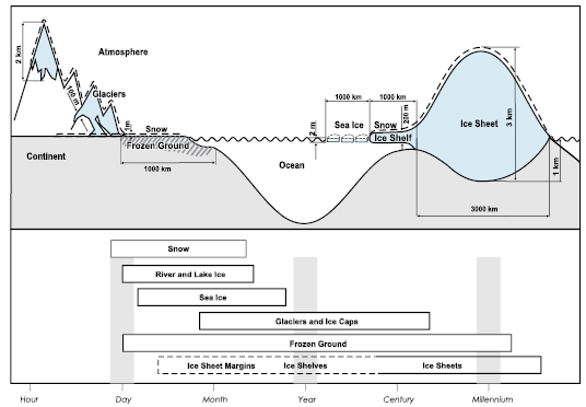
The main components of the cryosphere are snow, river and lake ice, sea ice, glaciers and ice caps, ice shelves, ice sheets, and frozen ground( Figure 4.1 ). In terms of the ice mass and its heat capacity, the cryosphere is the second largest component of the climate system (after the ocean). Its relevance for climate variability and change is based on physical properties, such as its high surface reflectivity (albedo) and the latent heat associated with phase changes, which have a strong impact on the surface energy balance. The presence (absence) of snow or ice in polar regions is associated with an increased (decreased) meridional temperature difference, which affects winds and ocean currents. Because of the positive temperature-ice albedo feedback, some cryospheric components act to amplify both changes and variability. However, some, like glaciers and permafrost, act to average out short-term variability and so are sensitive indicators of climate change. Elements of the cryosphere are found at all latitudes, enabling a near-global assessment of cryosphere-related climate changes.
The cryosphere on land stores about 75% of the world’s freshwater. The volumes of the Greenland and Antarctic Ice Sheets are equivalent to approximately 7 m and 57 m of sea level rise, respectively. Changes in the ice mass on land have contributed to recent changes in sea level. On a regional scale, many glaciers and ice caps play a crucial role in freshwater availability.
Presently, ice permanently covers 10% of the land surface, of which only a tiny fraction lies in ice caps and glaciers outside Antarctica and Greenland( Table 4.1 ). Ice also covers approximately 7% of the oceans in the annual mean. In midwinter, snow covers approximately 49% of the land surface in the Northern Hemisphere (NH). Frozen ground has the largest area of any component of the cryosphere. Changes in the components of the cryosphere occur at different time scales, depending on their dynamic and thermodynamic characteristics( Figure 4.1 ). All parts of the cryosphere contribute to short-term climate changes, with permafrost, ice shelves and ice sheets also contributing to longer-term changes including the ice age cycles.
Table 4.1: Area, volume and sea level equivalent (SLE) of cryospheric components. Indicated are the annual minimum and maximum for snow, sea ice and seasonally frozen ground, and the annual mean for the other components. The sea ice area is represented by the extent (area enclosed by the sea ice edge). The values for glaciers and ice caps denote the smallest and largest estimates excluding glaciers and ice caps surrounding Greenland and Antarctica.
| Cryospheric Component | Area | Ice Volume (106 km2) | Potential Sea Level Rise (SLE) (m)g |
|---|---|---|---|
| Snow on land (NH) | 1.9–45.2 | 0.0005–0.005 | 0.001–0.01 |
| Sea ice | 19–27 | 0.019–0.025 | ~0 |
| Glaciers and ice caps | |||
| Smallest estimatea | 0.51 | 0.05 | 0.15 |
| Largest estimateb | 0.54 | 0.13 | 0.37 |
| Ice shelvesc | 1.5 | 0.7 | ~0 |
| Ice sheets | 14.0 | 27.6 | 63.9 |
| Greenlandd | 1.7 | 2.9 | 7.3 |
| Antarcticac | 12.3 | 24.7 | 56.6 |
| Seasonally frozen ground (NH)e | 5.9–48.1 | 0.006–0.065 | ~0 |
| Permafrost (NH)f | 22.8 | 0.011–0.037 | 0.03–0.10 |
Seasonally, the area covered by snow in the NH ranges from a mean maximum in January of 45.2 × 10⁶ km2 to a mean minimum in August of 1.9 × 10⁶ km2 ( 1966 – 2004 ). Snow covers more than 33% of lands north of the equator from November to April, reaching 49% coverage in January. The role of snow in the climate system includes strong positive feedbacks related to albedo and other, weaker feedbacks related to moisture storage, latent heat and insulation of the underlying surface (M.P. Clark et al., 1999 [Ambiguous] ), which vary with latitude and season.
High-latitude rivers and lakes develop an ice cover in winter. Although the area and volume are small compared to other components of the cryosphere, this ice plays an important role in freshwater ecosystems, winter transportation, bridge and pipeline crossings, etc. Changes in the thickness and duration of these ice covers can therefore have consequences for both the natural environment and human activities. The breakup of river ice is often accompanied by ‘ice jams’ (blockages formed by accumulation of broken ice); these jams impede the flow of water and may lead to severe flooding.
At maximum extent arctic sea ice covers more than 15 × 106 km2,reducing to only 7 × 10⁶ km2 in summer. Antarctic sea ice is considerably more seasonal, ranging from a winter maximum of over 19 × 106 km2 to a minimum extent of about 3 × 10⁶ km2.Sea ice less than one year old is termed ‘first-year ice’ and that which survives more than one year is called ‘multi-year ice’. Most sea ice is part of the mobile ‘pack ice’, which circulates in the polar oceans, driven by winds and surface currents. This pack ice is extremely inhomogeneous, with differences in ice thicknesses and age, snow cover, open water distribution, etc. occurring at spatial scales from metres to hundreds of kilometres.
Glaciers and ice caps adapt to a change in climate conditions much more rapidly than does a large ice sheet, because they have a higher ratio between annual mass turnover and their total mass. Changes in glaciers and ice caps reflect climate variations, in many cases providing information in remote areas where no direct climate records are available, such as at high latitudes or on the high mountains that penetrate high into the middle troposphere. Glaciers and ice caps contribute to sea level changes and affect the freshwater availability in many mountains and surrounding regions. Formation of large and hazardous lakes is occurring as glacier termini retreat from prominent Little Ice Age moraines, especially in the steep Himalaya and Andes.
The ice sheets of Greenland and Antarctica are the main reservoirs capable of affecting sea level. Ice formed from snowfall spreads under gravity towards the coast, where it melts or calves into the ocean to form icebergs. Until recently (including IPCC, 2001 [NPR] ) it was assumed that the spreading velocity would not change rapidly, so that impacts of climate change could be estimated primarily from expected changes in snowfall and surface melting. Observations of rapid ice flow changes since IPCC 2001 [NPR] ) have complicated this picture, with strong indications that floating ice shelves ‘regulate’ the motion of tributary glaciers, which can accelerate manyfold following ice shelf breakup.
Frozen ground includes seasonally frozen ground and permafrost. The permafrost region occupies approximately 23 × 106 km2 or 24% of the land area in the NH. On average, the long-term maximum areal extent of the seasonally frozen ground, including the active layer over permafrost, is about 48 × 106 km2 or 51% of the land area in the NH. In terms of areal extent, frozen ground is the single largest cryospheric component. Permafrost also acts to record air temperature and snow cover variations, and under changing climate can be involved in feedbacks related to moisture and greenhouse gas exchange with the atmosphere.
4.2 Changes in Snow Cover
4.2.1 Background
The high albedo of snow (0.8 to 0.9 for fresh snow) has an important influence on the surface energy budget and on Earth’s radiative balance (e.g., Groisman et al., 1994 [PoC, JoC, ARC] ). Snow albedo, and hence the strength of the feedback, depends on a number of factors such as the depth and age of a snow cover, vegetation height, the amount of incoming solar radiation and cloud cover. The albedo of snow may be decreasing because of anthropogenic soot ( Hansen and Nazarenko, 2004 [JoC, MoS, ARC] ; see Section 2.5.4 for details).
In addition to the direct snow-albedo feedback, snow may influence climate through indirect feedbacks (i.e., those in which there are more than two causal steps), such as to summer soil moisture. Indirect feedbacks to atmospheric circulation may involve two types of circulation, monsoonal (e.g., Lo and Clark, 2001 [JoC] ) and annular (e.g., Saito and Cohen, 2003 [JoC, MoS] ; see Section 3.6.4 ), although there are large uncertainties in the physical mechanisms involved ( Bamzai, 2003 [JoC] ; Robock et al., 2003 [JoC, SRC] ).
In this section, observations of snow cover extent are updated from IPCC 2001 [NPR] ). In addition, several new topics are covered: changes in snow depth and snow water equivalent; relationships of snow to temperature and precipitation; and observations and estimates of changes in snow in the Southern Hemisphere (SH). Changes in the fraction of precipitation falling as snow or other frozen forms are covered in Section 3.3.2.3 .This section covers only snow on land; snow on various forms of ice is covered in subsequent sections.
4.2.2 Observations of Snow Cover, Snow Duration and Snow Quantity
4.2.2.1 Sources of Snow Data
Daily observations of the depth of snow and of new snowfall have been made by various methods in many countries, dating to the late 1800 s in a few countries (e.g., Switzerland, USA, the former Soviet Union and Finland). Measurements of snow depth and snow water equivalent (SWE) became widespread by 1950 in the mountains of western North America and Europe, and a few sites in the mountains of Australia have been monitored since 1960 . In situ snow data are affected by changes in station location, observing practices and land cover, and are not uniformly distributed.
The premier data set used to evaluate large-scale snow covered area (SCA), which dates to 1966 and is the longest satellite-derived environmental data set of any kind, is the weekly visible wavelength satellite maps of NH snow cover produced by the US National Oceanic and Atmospheric Administration’s (NOAA) National Environmental Satellite Data and Information Service (NESDIS; Robinson et al., 1993 [JoC, SRC] ). Trained meteorologists produce the weekly NESDIS snow product from visual analyses of visible satellite imagery. These maps are well validated against surface observations, although changes in mapping procedures in 1999 affected the continuity of data series at a small number of mountain and coastal grid points. For the SH, mapping of SCA began only in 2000 with the advent of Moderate Resolution Imaging Spectroradiometer (MODIS) satellite data.
Space-borne passive microwave sensors offer the potential for global monitoring since 1978 of not just snow cover, but also snow depth and SWE, unimpeded by cloud cover and winter darkness. In order to generate homogeneous depth or SWE data series, differences between Scanning Multichannel Microwave Radiometer (SMMR; 1978 to 1987 ) and Special Sensor Microwave/Imager (SSM/I; 1987 to present) in 1987 must be resolved ( Derksen et al., 2003 [JoC] ). Estimates of SCA from microwave satellite data compare moderately well with visible data except in autumn (when microwave estimates are too low) and over the Tibetan plateau (microwave too high; Armstrong and Brodzik, 2001 [JoC] ). Work is ongoing to develop reliable depth and SWE retrievals from passive microwave for areas with heavy forest or deep snowpacks, and the relatively coarse spatial resolution (~10–25 km) still limits applications over mountainous regions.
4.2.2.2 Variability and Trends in Northern Hemisphere Snow Cover
In this subsection, following the hemispheric view provided by the large-scale analyses by Brown 2000 [JoC, SRC] and Robinson et al. 1993 [JoC, SRC] ), regional and national-scale studies are discussed. The mean annual NH SCA ( 1966 – 2004 ) is 23.9 × 10⁶ km2,not including the Greenland Ice Sheet. Interannual variability of SCA is largest not in winter, when mean SCA is greatest, but in autumn (in absolute terms) or summer (in relative terms). Monthly standard deviations range from 1.0 × 10⁶ km2 in August and September to 2.7 × 10⁶ km2 in October, and are generally just below 2 × 10⁶ km2 in non-summer months.
Since the early 1920 s, and especially since the late 1970 s, SCA has declined in spring( Figure 4.2 )and summer, but not substantially in winter( Table 4.2 )despite winter warming (see Section 3.2.2 ). Recent declines in SCA in the months of February through August have resulted in (1) a shift in the month of maximum SCA from February to January; (2) a statistically significant decline in annual mean SCA; and (3) a shift towards earlier spring melt by almost two weeks in the 1972 to 2000 period ( (Dye, 2002 ) ). Early in the satellite era, between 1967 and 1987, mean annual SCA was 24.4 × 10⁶ km2.An abrupt transition occurred between 1986 and 1988, and since 1988 the mean annual extent has been 23.1 × 10⁶ km2,a statistically significant (T test, p <0.01) reduction of approximately 5% ( Robinson and Frei, 2000 [SRC] ). Over the longer 1922 to 2005 period (updated from Brown, 2000 [JoC, SRC] ), the linear trend in March and April NH SCA( Figure 4.2 )is a statistically significant reduction of 2.7 ± 1.5 × 10⁶ km2 or 7.5 ± 3.5%.
Table 4.2. Trend (106 km2 per decade) in monthly NH SCA from satellite data (Rutgers-corrected, D. Robinson) over the 1966 to 2005 period and for three months covering the 1922 to 2005 period based on the NH SCA reconstruction of Brown 2000 [JoC, SRC] ).
| Years | Jan | Feb | Mar | Apr | May | Jun | Jul | Aug | Sep | Oct | Nov | Dec | Ann |
|---|---|---|---|---|---|---|---|---|---|---|---|---|---|
| 1966–2005 | –0.11 | –0.49 | –0.80a | –0.74a | –0.57 | –1.10a | –1.17a | –0.82a | –0.20 | –0.36 | 0.12 | 0.19 | –0.33a |
| 1922–2005 | n/a | n/a | –0.25a | –0.35a | n/a | n/a | n/a | n/a | n/a | 0.24a | n/a | n/a | n/a |
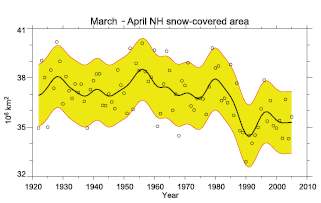
Figure 4.2. Update of NH March-April average snow-covered area (SCA) from Brown 2000 [JoC, SRC] ). Values of SCA before 1972 are based on the station-derived snow cover index of Brown 2000 [JoC, SRC] ); values beginning in 1972 are from the NOAA satellite data set. The smooth curve shows decadal variations (see Appendix 3.A ), and the shaded area shows the 5 to 95% range of the data estimated after first subtracting the smooth curve.
Temperature variations and trends play a significant role in variability and trends of NH SCA, by determining whether precipitation falls as rain or snow, and by determining snowmelt. In almost every month, SCA is correlated with temperature in the latitude band of greatest variability in SCA, owing to the snow-albedo feedback. For example, temperature in the 40°N to 60°N band and NH SCA are highly correlated in spring (r = –0.68; updated from Brown, 2000 [JoC, SRC] ) and the largest reductions in March-April average snow cover occurred roughly between the 0°C and 5°C isotherms( Figure 4.3 ). The snow-albedo feedback also helps determine the longer-term trends (for temperature see Section 3.2.2 ;see also M.P. Clark et al., 1999 [Ambiguous] ; Groisman et al., 1994 [PoC, JoC, ARC] ).
The following paragraphs discuss regional details, including information not available or missing from the satellite data and from Brown’s ( 2000 ) hemispheric reconstruction.
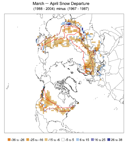
Figure 4.3. Differences in the distribution of Northern Hemisphere March-April average snow cover between earlier ( 1967 – 1987 ) and later ( 1988 – 2004 ) portions of the satellite era (expressed in % coverage). Negative values indicate greater extent in the earlier portion of the record. Extents are derived from NOAA/NESDIS snow maps. Red curves show the 0°C and 5°C isotherms averaged for March and April 1967 to 2004, from the Climatic Research Unit (CRU) gridded land surface temperature version 2 (CRUTEM2v) data.
4.2.2.2.1 North America
From 1915 to 2004, North American SCA increased in November, December and January owing to increases in precipitation( Section 3.3.2 ;Groisman et al., 2004 [JoC, ARC] ). Decreases in snow cover are mainly confined to the latter half of the 20th century, and are most apparent in the spring period over western North America ( Groisman et al., 2004 [JoC, ARC] ). Shifts towards earlier melt by about eight days since the mid- 1960 s were also observed in northern Alaska ( Stone et al., 2002 [JoC] ).
Another dimension of change in snow is provided by the annual measurements of mountain SWE near April 1 in western North America, which indicate declines since 1950 at about 75% of locations monitored ( Mote et al., 2005 [JoC, SRC] ). The date of maximum mountain SWE appears to have shifted earlier by about two weeks since 1950, as inferred from streamflow measurements ( Stewart et al., 2005 [JoC, ARC] ). That these reductions are predominantly due to warming is shown by regression analysis of streamflow ( Stewart et al., 2005 [JoC, ARC] ) and SWE ( Mote, 2006 [JoC, SRC] ) on temperature and precipitation, and by the dependence of trends in SWE ( Mote et al., 2005 [JoC, SRC] ) on elevation or equivalently mean winter temperature( Figure 4.4 a), with the largest percentage changes near the 0°C level.
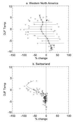
Figure 4.4. Dependence of trends in snow on mean winter temperature (°C) at each location. (a) Relative trends in 1 April SWE, 1950 to 2000, in the mountains of western North America (British Columbia, Washington, Oregon and California), binned by mean December to February (DJF) temperature. For each 1°C temperature bin, ‘×’ symbols indicate the mean trend, bars indicate the span of the 5 to 95% confidence interval for bins with at least 10 points, and circles indicate outliers. Total number of data points is 323 (adapted from Mote et al., 2005 [JoC, SRC] ). (b) Relative trend in days of winter (DJF) snow cover at 109 sites in Switzerland, 1958 to 1999, binned by mean DJF temperature (adapted from Scherrer et al., 2004 [JoC, SRC] ).
4.2.2.2.2 Europe and Eurasia
Snow cover trends in mountain regions of Europe are characterised by large regional and altitudinal variations. Recent declines in snow cover have been documented in the mountains of Switzerland (e.g., Scherrer et al., 2004 [JoC, SRC] ) and Slovakia ( (Vojtek et al., 2003 ) ), but no change was observed in Bulgaria over the 1931 to 2000 period ( (Petkova et al., 2004 ) ). Declines, where observed, were largest at lower elevations, and Scherrer et al. 2004 [JoC, SRC] ) statistically attributed the declines in the Swiss Alps to warming, as is clear when trends are plotted against winter temperature( Figure 4.4 b).
Lowland areas of central Europe are characterised by recent reductions in annual snow cover duration by about 1 day yr–1 (e.g., ( Falarz, 2002 ) ). Trends towards greater maximum snow depth but shorter snow season have been noted in Finland ( (Hyvärinen, 2003 ) ), the former Soviet Union from 1936 to 1995 ( Ye and Ellison, 2003 [JoC] ), and in the Tibetan Plateau ( Zhang et al., 2004 [JoC, ARC] ) since the late 1970 s. Qin et al. 2006 [JoC, SRC] ) reported no trends in snow depth or snow cover in western China since 1957 .
4.2.2.3 Southern Hemisphere
Outside of Antarctica (see Section 4.6 ), very little land area in the SH experiences snow cover. Long-term records of snow cover, snowfall, snow depth or SWE are scarce. In some cases, proxies for snow line can be used, but the quality of data is much lower than for most NH areas.
4.2.2.3.1 South America
Estimates from microwave satellite observations for mid-latitude alpine regions of South America for the period of record 1979 to 2002 show substantial interannual variability with little or no long-term trend. A long-term increasing trend in the number of snow days was found in the eastern side of the central Andes region (33°S) from 1885 to 1996, derived from newspaper reports of Mendoza City ( (Prieto et al., 2001 ) ).
Other approaches suggest some response of snow line to warming in South America. The 0°C isotherm altitude (ZIA), an indication of snow line, has been derived from the daily temperature profile obtained from radiosonde data located at Quintero (32°47’S, 71°33’W, 8 m above sea level; Carrasco et al., 2005 [SRC] ), which represents the snow line behaviour in the western Andes from about 30°S to 36°S. Over the 1975 to 2001 period of record, the linear change in winter ZIA was 121.9 ± 7.7 m, and the positive trend was dominated by atmospheric conditions on dry days (enhancing melt) with no trend on wet days (accumulation zone unchanged).
4.2.2.3.2 Australia and New Zealand
For the mountainous south-eastern area of Australia, studies of late winter (August–September) snow depth have shown some significant declines (as much as 40%) since 1962 . Trends in maximum snow depth were more modest. The stronger declines in late winter are attributed to spring season warming, while maximum snow depth is largely determined by winter precipitation, which has declined only slightly ( Hennessy et al., 2003 [NPR] ; Nicholls, 2005 [ARC] ).
In New Zealand, annual observations of end-of-summer snow line on 47 glaciers have been made by airplane since 1977, and reveal large interannual variability primarily associated with atmospheric circulation anomalies ( Clare et al., 2002 [JoC] ); it is noteworthy, however, that the four years with highest snow line occurred in the 1990 s. The only study of seasonal snow cover in the Southern Alps found no trend over the 1930 to 1985 period ( Fitzharris and Garr, 1995 [MoS, SRC] ) and has not been updated.
4.3 Changes in River and Lake Ice
4.3.1 Background
Because of its importance to many human activities, freeze-up and breakup dates of river and lake ice have been recorded for a long time at many locations. These records provide useful climate information, although they must be interpreted with care. In the case of rivers, both freeze-up and breakup at a given location can be strongly affected by conditions far upstream (for example, heavy rains or snowmelt in a distant portion of the watershed). In the case of lakes, the historical observations have typically been made at coastal locations (often protected bays and harbours) and so may not be representative of the lake as a whole, or comparable to more recent satellite-based observations. Nevertheless, these observations represent some of the longest records of cryospheric change available.
Observations of ice thickness are considerably sparser and are generally made using direct drilling methods. Long-term records are available at a few locations; however it should be noted that, just as for sea ice, changes in lake and river ice thickness are a consequence not just of temperature and radiative forcing, but also of changes in snowfall (via the insulating effect of snow).
4.3.2 Changes in Freeze-up and Breakup Dates
Freeze-up is defined conceptually as the time at which a continuous and immobile ice cover forms; however, operational definitions range from local observations of the presence or absence of ice to inferences drawn from river discharge measurements. Breakup is typically the time when the ice cover begins to move downstream in a river or when open water becomes extensive at the measurement location for lakes. Here again, there is some ambiguity in the specific date, and in the extent to which local observations reflect conditions elsewhere on a large lake or in a large river basin.
Selected time series from a recent compilation of river and lake freeze-up and breakup records by Magnuson et al. 2000 [JoC] ) are shown in Figure 4.5 .They limited consideration to records spanning at least 150 years. Eleven out of 15 records showed significant trends towards later freeze-up and 17 out of 25 records showed significant trends towards earlier breakup. When averaged together, the freeze-up date has become later at a rate of 5.8 ± 1.6 days per century, while the breakup date has occurred earlier at a rate of 6.5 ± 1.2 days per century.
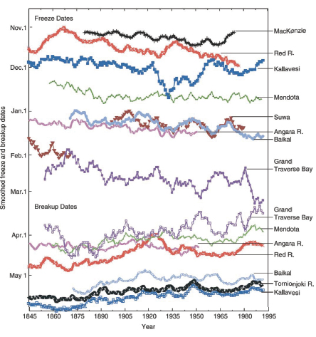
Figure 4.5. Time series of freeze-up and breakup dates from several northern lakes and rivers (reprinted with permission from Magnuson et al., 2000 [JoC] , copyright AAAS). Dates have been smoothed with a 10-year moving average. See the cited publication for locations and other details.
Alarger sample of Canadian rivers spanning the last 30 to 50 years was analysed by Zhang et al. 2001 [ARC] ). These freeze-up and breakup estimates (based on inferences from streamflow data) exhibit considerable variability, with a trend towards earlier freeze-up and breakup over much of the country. The earlier freeze-up dominates, however, leading to a significant decrease in open water duration at many locations as shown in Figure 4.6 .A recent analysis of Russian river data by ( Smith 2000 ) ) revealed a trend towards earlier freeze-up of western Russian rivers and later freeze-up in rivers of eastern Siberia over the last 50 to 70 years. Breakup dates did not exhibit statistically significant trends.
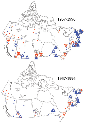
Figure 4.6. Trends in river ice cover duration in Canada. Upward pointing triangles indicate lengthening of the ice cover period while downward triangles indicate shortening of the ice cover period. Trends significant at the 99 and 90% confidence levels are marked by larger filled and hollow triangles, respectively. Smaller triangles indicate trends that are not significant at the 90% level ( Zhang et al., 2001 [ARC] ).
Acomparable analysis of freeze-up and breakup dates for Canadian lakes has recently been completed by ( Duguay et al. 2006 ) ). These results (shown in Figure 4.7 )indicate a fairly general trend towards earlier breakup (particularly in western Canada), while freeze-up exhibited a mix of early and later dates.
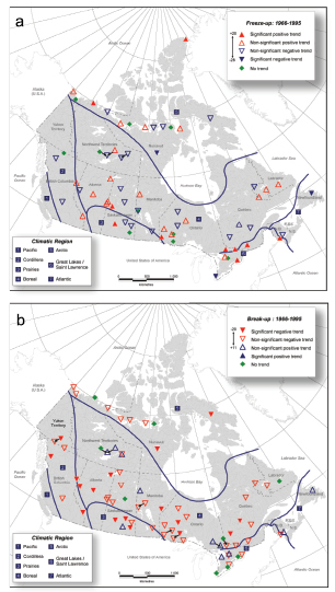
Figure 4.7. Trends in (a) freeze-up and (b) breakup dates observed at lakes in Canada over the period 1965 to 1995 . Downward pointing arrows indicate a trend towards earlier dates; upward pointing arrows, a trend towards later dates. Open symbols indicate that the trend is not significant while solid symbols indicate that the trend is significant at the 90% confidence level (modified from ( Duguay et al., 2006 ) ).
There are insufficient published data on river and lake ice thickness to allow assessment of trends. Modelling studies (e.g., Duguay et al., 2003 [MoS] ) indicate that, as with the landfast sea ice case, much of the variability in maximum ice thickness and breakup date is driven by variations in snowfall.
4.4 Changes in Sea Ice
4.4.1 Background
Sea ice is formed by freezing of seawater in the polar oceans. It is an important, interactive component of the global climate system because: a) it is central to the powerful ‘ice-albedo’ feedback mechanism that enhances climate response at high latitudes (see Chapter2 ); b) it modifies the exchange of heat, gases and momentum between the atmosphere and polar oceans; and c) it redistributes freshwater via the transport and subsequent melt of relatively fresh sea ice, and hence alters ocean buoyancy forcing.
The thickness of sea ice is a consequence of past growth, melt and deformation, and so is an important indicator of climatic conditions. Ice thickness is also closely connected to ice strength, and so changes in thickness are important to navigability by ships, to the stability of the ice as a platform for use by humans and marine mammals, to light transmission through the ice cover, etc. Sea ice increases in thickness as bottom freezing balances heat conduction through the ice to the surface (heat conduction is strongly influenced by the insulating thickness of the ice itself and the snow on it). Most of the inhomogeneity in the pack results from deformation of the ice due to differential movement of individual pieces of ice (called ‘floes’). Open water areas created within the ice pack under divergence or shear (called ‘leads’) are a major contributor to ocean-atmosphere heat exchange (turbulent heat loss from the ocean in winter and shortwave heating in the summer). In some locations, due either to persistent ice divergence or to persistent upwelling of oceanic heat, open water areas within an otherwise ice-covered region can be sustained over much of the winter. These are called ‘polynyas’ and are important feeding areas for marine mammals and birds.
Under convergence, thin ice sheets may ‘raft’ on top of each other, doubling the ice thickness, and under strong convergence (for example, when wind drives sea ice against a coast), the ice buckles and crushes to form sinuous ‘ridges’ of thick ice. In the Arctic, ridges can be tens of metres thick, account for nearly half of the total ice volume and constitute a major impediment to transportation on, through, or under the ice. Although ridging is generally less severe in the Antarctic, ice deformation is still an important process in thickening the ice cover.
Near the shore, in bays and fjords, and among islands like those of the Canadian Arctic Archipelago, sea ice can be attached to land and therefore be immobile. This is termed ‘landfast’ ice. In the Arctic such ice (and in particular its freeze-up and breakup) is of special importance to local residents as it is used as a platform for hunting and fishing, and is an impediment to shipping.
Some climatically important characteristics of sea ice include: its concentration (that fraction of the ocean covered by ice); its extent (the area enclosed by the ice edge – operationally defined as the 15% concentration contour); the total area of ice within its extent (i.e., extent weighted by concentration); the area of multi-year ice within the total extent; its thickness (and the thickness of the snow cover on it); its velocity; and its growth and melt rates (and hence salt or freshwater flux into the ocean). Ice extent, or ice edge position, is the only sea ice variable for which observations are available for more than a few decades. Expansion or retreat of the ice edge may be amplified by the ice-albedo feedback.
4.4.2 Sea Ice Extent and Concentration
4.4.2.1 Data Sources and Time Periods Covered
The most complete record of sea ice extent is provided by passive microwave data from satellites that are available since the early 1970 s. Prior to that, aircraft, ship and coastal observations are available at certain times and in certain locations. Portions of the North Atlantic are unique in having ship observations extending well back into the 19th century. Far fewer historic data exist from the SH, with one notable exception being the record of annual landfast ice duration from the sub-antarctic South Orkney islands starting in 1903 ( (Murphy et al., 1995 ) ).
Estimation of sea ice properties from passive microwave emission requires an algorithm to convert observed radiance into ice concentration (and type). Several such algorithms are available (e.g., Steffen et al., 1992 [NPR, MoS] ) and their accuracy has been evaluated using high-resolution satellite and aircraft imagery (e.g., Cavalieri, 1992 [NPR] ; Kwok, 2002 [JoC, SRC] ) and operational ice charts (e.g., ( Agnew and Howell, 2003 ) ). The accuracy of satellite-derived ice concentration is usually 5% or better, although errors of 10 to 20% can occur during the melt season. The accuracy of the ice edge (relevant to estimating ice extent) is largely determined by the spatial resolution of the satellite radiometer, and is of the order of 25 km (recently launched instruments provide improved resolution of about 12.5 km). Summer concentration errors do lead to a bias in estimated ice-covered area in both the NH and SH warm seasons ( (Agnew and Howell, 2003; ) Worby and Comiso, 2004 [SRC] ). This is an important consideration when comparing the satellite period with older proxy records of ice extent.
Distinguishing between first-year and multi-year ice from passive microwave data is more difficult, although algorithms are improving (e.g., Johannessen et al., 1999 [JoC] ). However, the summer minimum ice extent, which is by definition the multi-year ice extent at that time of year, is not as prone to algorithm errors (e.g., Comiso, 2002 [JoC, SRC] ).
4.4.2.2 Hemispheric, Regional and Seasonal Time Series from Passive Microwave
Most analyses of variability and trend in ice extent using the satellite record have focussed on the period after 1978 when the satellite sensors have been relatively constant. Different estimates, obtained using different retrieval algorithms, produce very similar results for hemispheric extent, and all show an asymmetry between changes in the Arctic and Antarctic. As an example, an updated version of the analysis done by Comiso 2003 [NPR, SRC] ), spanning the period from November 1978 through December 2005, is shown in Figure 4.8 .The annual mean ice extent anomalies are shown. There is a significant decreasing trend in arctic sea ice extent of –33 ± 7.4 × 10³ km2 yr–1 (equivalent to –2.7 ± 0.6% per decade), whereas the antarctic results show a small positive trend of 5.6 ± 9.2 × 10³ km2 yr–1 (0.47 ± 0.8% per decade), which is not statistically significant. The uncertainties represent the 90% confidence interval around the trend estimate and the percentages are based on the 1978 to 2005 mean. In both hemispheres, the trends are larger in summer and smaller in winter. In addition, there is considerable variation in the magnitude, and even the sign, of the trend from region to region within each hemisphere.
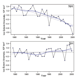
Figure 4.8. Sea ice extent anomalies (computed relative to the mean of the entire period) for (a) the NH and (b) the SH, based on passive microwave satellite data. Symbols indicate annual mean values while the smooth blue curves show decadal variations (see Appendix 3.A ). Linear trend lines are indicated for each hemisphere. For the Arctic, the trend is –33 ± 7.4 × 10³ km2 yr–1 (equivalent to approximately –2.7% per decade), whereas the Antarctic results show a small positive trend of 5.6 ± 9.2 × 10³ km2 yr–1.The negative trend in the NH is significant at the 90% confidence level whereas the small positive trend in the SH is not significant (updated from Comiso, 2003 [NPR, SRC] ).
The most remarkable change observed in the arctic ice cover has been the decrease in ice that survives the summer, shown in Figure 4.9 .The trend in the minimum arctic sea ice extent, between 1979 and 2005, was –60 ± 20 × 103 km2 yr–1 (–7.4 ± 2.4% per decade). These trends are superimposed on substantial interannual to decadal variability, which is associated with variability in atmospheric circulation ( Belchansky et al., 2005 [JoC] ).
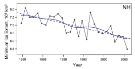
Figure 4.9. Summer minimum arctic sea ice extent from 1979 to 2005 . Symbols indicate annual mean values while the smooth blue curve shows decadal variations (see Appendix 3.A ). The dashed line indicates the linear trend, which is –60 ± 20 × 103 km2 yr–1,or approximately –7.4% per decade (updated from Comiso, 2002 [JoC, SRC] ).
4.4.2.3 Longer Records of Hemispheric Extent
The lack of comprehensive sea ice data prior to the satellite era hampers estimates of hemispheric-scale trends over longer time scales. Rayner et al. 2003 [JoC] ) compiled a data set of sea ice extent for the 20th century from available sources and accounted for the inhomogeneity between them( Figure 4.10 ). There is a clear indication of sustained decline in arctic ice extent since about the early 1970 s, particularly in summer. On a regional basis, portions of the North Atlantic have sufficient historical data, based largely on ship reports and coastal observations, to permit trend assessments over periods exceeding 100 years. Vinje 2001 [JoC] ) compiled information from ship reports in the Nordic Seas to estimate April sea ice extent in this region for the period since about 1860 . This time series is also shown in Figure 4.10 and indicates a generally continuous decline from the start of the record to the end. Ice extent data from Russian sources have recently been published ( Polyakov et al., 2003 [JoC] ), and cover essentially the entire 20th century for the Russian coastal seas (Kara, Laptev, East Siberian and Chukchi). These data, which exhibit large inter-decadal variability, show a declining trend since the 1960 s until a reversal in the late 1990 s. The Russian data indicate anomalously little ice during the 1940 s and 1950 s, whereas the Nordic Sea data indicate anomalously large extent at this time, showing the importance of regional variability.
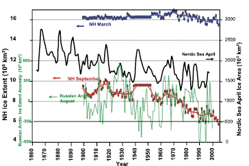
Figure 4.10. Time series of NH sea ice extent for March and September from the Hadley Centre Sea Ice and Sea Surface Temperature (HadISST) data set (the blue and red curves, updated from Rayner et al., 2003 [JoC] ), the April Nordic Sea ice extent (the black curve, redrafted from Vinje, 2001 [JoC] ) and the August ice extent anomaly (computed relative to the mean of the entire period) in the Russian Arctic seas – Kara, Laptev, East Siberian and Chukchi (dotted green curve, redrafted from Polyakov et al., 2003 [JoC] ). For the NH time series, the symbols indicate yearly values while the curves show the decadal variation (see Appendix 3.A ).
Omstedt and Chen 2001 [JoC] ) obtained a proxy record of the annual maximum extent of sea ice in the region of the Baltic Sea over the period 1720 to 1997 . This record showed a substantial decline in sea ice that occurred around 1877, and greater variability in sea ice extent in the colder 1720 to 1877 period than in the warmer 1878 to 1997 period. Hill et al. 2002 [NPR] ) have examined sea ice information for the Canadian maritime region and deduced that sea ice incursions occurred during the 19th century in the Grand Banks and surrounding areas that are now ice-free. Although there are problems with homogeneity of all these data (with quality declining further back in history), and with the disparity in spatial scales represented by each, they are all consistent in terms of the declining ice extent during the latter decades of the 20th century, with the decline beginning prior to the satellite era. Those data that extend far enough back in time imply, with high confidence, that sea ice was more extensive in the North Atlantic during the 19th century.
Continuous long-term data records for the Antarctic are lacking, as systematic information on the entire Southern Ocean ice cover became available only with the advent of routine microwave satellite reconnaissance in the early 1970 s. ( Parkinson 1990 ) ) examined ice edge observations from four exploration voyages in the late 18th and early 19th centuries. Her analysis suggested that the summer antarctic sea ice was more extensive in the eastern Weddell Sea in 1772 and in the Amundsen Sea in 1839 than the present day range from satellite observations. However, many of the early observations are within the present range for the same time of year. An analysis of whaling records by de la Mare 1997 [JoC] ) suggested a step decline in antarctic sea ice coverage of 25% (a 2.8° poleward shift in average ice edge latitude) between the mid- 1950 s and the early 1970 s. A reanalysis by Ackley et al. 2003 [SRC] ), which accounted for offsets between satellite-derived ice edge and whaling ship locations, challenged evidence of significant change in ice edge location. Curran et al. 2003 [JoC] ) made use of a correlation between methanesulphonic acid concentration (a by-product of marine phytoplankton) in a near-coastal antarctic ice core and the regional sea ice extent in the sector from 80°E to 140°E to infer a quasi-decadal pattern of interannual variability in the ice extent in this region, along with a roughly 20% decline (approximately two degrees of latitude) since the 1950 s.
In summary, the antarctic data provide evidence of a decline in sea ice extent in some regions, but there are insufficient data to draw firm conclusions about hemispheric changes prior to the satellite era.
4.4.3 Sea Ice Thickness
4.4.3.1 Sea Ice Thickness Data Sources and Time Periods Covered
Until recently there have been no satellite remote sensing techniques capable of mapping sea ice thickness, and this parameter has primarily been determined by drilling or by under-ice sonar measurement of draft (the submerged portion of sea ice).
Subsea sonar from submarines or moored instruments can be used to measure ice draft over a footprint of 1 to 10 m diameter. Draft is converted to thickness, assuming an average density for the measured floe, including its snow cover. The principal challenges to accurate observation with sonar are uncertainties in sound speed and atmospheric pressure, and the identification of spurious targets. Upward-looking sonar has been on submarines operating beneath arctic pack ice since 1958 . US and UK naval data are now being released for science, and some dedicated arctic submarine missions were made for science during 1993 to 1999 . Ice draft measurement by moored ice-profiling sonar, best suited to studies of ice transport or change at fixed sites, began in the Arctic in the late 1980 s. Instruments have operated since 1990 in the Beaufort and Greenland Seas and for shorter intervals in other areas, but few records span more than 10 years. In the SH there are no data from submarines and only short time series from moored sonar.
Other techniques, such as electromagnetic induction sounders deployed on the ice surface, ships or aircraft, or airborne laser altimetry to measure freeboard (the portion of sea ice above the waterline), have limited applicability to wide-scale climate analysis of sea ice thickness. Indirect estimates, based on measurement of surface gravity waves, are available in some regions for the 1970 s and 1980 s ( (Nagurnyi et al., 1999 ) as reported in Johannessen et al., 2004 [JoC, MoS] ), but the accuracy of these estimates is difficult to quantify.
Quantitative data on the thickness of antarctic pack ice only started to become available in the 1980 s from sparsely scattered drilling programs covering only small areas and primarily for use in validating other techniques. Visual observations of ice characteristics from ships ( Worby and Ackley, 2000 [JoC, SRC] ) are not adequate for climate monitoring, but are providing one of the first broad pictures of antarctic sea ice thickness.
4.4.3.2 Evidence of Changes in Arctic Pack Ice Thickness from Submarine Sonar
Estimates of thickness change over limited regions are possible when submarine transects are repeated (e.g., Wadhams, 1992 [JoC] ). The North Pole is a common waypoint in many submarine cruises and this allowed McLaren et al. 1994 [NPR, SRC] ) to analyse data from 12 submarine cruises near the pole between 1958 and 1992 . They found considerable interannual variability, but no significant trend. Shy and Walsh 1996 [JoC, SRC] ) examined the same data in relation to ice drift and found that much of the thickness variability was due to the source location and path followed by the ice prior to arrival at the pole.
Rothrock et al. 1999 [JoC, SRC] ) provided the first ‘basin-scale’ analysis and found that ice draft in the mid- 1990 s was less than that measured between 1958 and 1977 at every available location (including the North Pole). The change was least (–0.9 m) in the southern Canada Basin and greatest (–1.7 m) in the Eurasian Basin (with an estimated overall error of less than 0.3 m). The decline averaged about 42% of the average 1958 to 1977 thickness. Their study included very few data within the seasonal sea ice zone and none within 300 km of Canada or Greenland.
Subsequent studies indicate that the reduction in ice thickness was not gradual, but occurred abruptly before 1991 Winsor 2001 [JoC] ) found no evidence of thinning along 150°W from six spring cruises during 1991 to 1996, but Tucker et al. 2001 [JoC] ), using spring observations from 1976 to 1994 along the same meridian, noted a decrease in ice draft sometime between the mid- 1980 s and early 1990 s, with little subsequent change. The observed change in mean draft resulted from a decrease in the fraction of thick ice (draft of more than 3.5 m) and an increase in the fraction of thin ice, which was probably due to reduced storage of multi-year ice in a smaller Beaufort Gyre and the export of ‘surplus’ via Fram Strait. Yu et al. 2004 [JoC, SRC] ) presented evidence of a similar change in ice thickness over a wider area. However, ice thickness varies considerably from year to year at a given location and so the rather sparse temporal sampling provided by submarine data makes inferences regarding long-term change difficult.
4.4.3.3 Other Evidence of Sea Ice Thickness Change in the Arctic and Antarctic
Haas 2004 [JoC, SRC] , and references therein) used ground-based electromagnetic induction measurements to show a decrease of approximately 0.5 m between 1991 and 2001 in the modal thickness (i.e., the most commonly observed thickness) of ice floes in the Arctic Trans-Polar Drift. Their survey of 120 km of ice on 146 floes during four cruises is biased by an absence of ice-free and thin-ice fractions and underestimation of ridged ice, but the data are descriptive of floes that are safe to traverse in summer, and the observed changes are most likely due to thermodynamic forcing.
An emerging new technique, using satellite radar or laser altimetry to estimate ice freeboard from the measured ranges to the ice and sea surface in open leads (and assuming an average floe density and snow depth), offers promise for future monitoring of large-scale sea ice thickness. Laxon et al. 2003 [JoC, SRC] ) estimated average arctic sea ice thickness over the cold months (October–March) for 1993 to 2001 from satellite-borne radar altimeter measurements. Their data reveal a realistic geographic variation in thickness (increasing from about 2 m near Siberia to 4.5 m off the coasts of Canada and Greenland) and a significant (9%) interannual variability in winter ice thickness, but no indication of a trend over this time.
There are no available data on change in the thickness of antarctic sea ice, much of which is considerably thinner and less ridged than ice in the Arctic Basin.
4.4.3.4 Model-Based Estimates of Change
Physically based sea ice models, forced with winds and temperatures from atmospheric reanalyses and sometimes constrained by observed ice concentration fields, can provide continuous time series of sea ice extent and thickness that can be compared to the sparse observations, and used to interpret the observational record. Models such as those described by Rothrock et al. 2003 [JoC, MoS, SRC] ) and references therein are able to reproduce the observed interannual variations in ice thickness, at least when averaged over fairly large regions. In particular, model studies can elucidate some of the forcing agents responsible for observed changes in ice thickness.
Acomparison of various model simulations of historical arctic ice thickness or volume is shown in Figure 4.11 .All the models indicate a marked reduction in ice thickness of 0.6 to 0.9 m starting in the late 1980 s, but disagree somewhat with respect to trends and/or variations earlier in the century. Most models indicate a maximum in ice thickness in the mid- 1960 s, with local maxima around 1980 and 1990 as well. There is an emerging suggestion from both models and observations that much of the decrease in thickness occurred between the late 1980 s and late 1990 s.
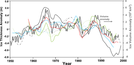
Figure 4.11. Comparison of model-based time series of the annual mean average sea ice thickness anomaly (computed relative to the mean of the entire period) in the Arctic Basin, obtained from a variety of models (redrafted from Rothrock et al., 2003 [JoC, MoS, SRC] ; see this paper for identification of the individual models and their attributes), along with the sea ice volume anomalies in the Arctic Basin (grey curve and right-hand scale; computed by Koeberle and Gerdes, 2003 [JoC, ARC] ).
It is not possible to attribute the abrupt decrease in thickness inferred from submarine observations entirely to the (rather slow) observed warming in the Arctic, and some of the dramatic decrease may be a consequence of spatial redistribution of ice volume over time (e.g., Holloway and Sou, 2002 [JoC] ). Low-frequency, large-scale modes of atmospheric variability (such as interannual changes in circulation connected to the Northern Annular Mode) affect both wind-driving of sea ice and heat transport in the atmosphere, and therefore contribute to interannual variations in ice formation, growth and melt (e.g., Rigor et al., 2002 [JoC, SRC] ; Dumas et al., 2003 [JoC, MoS, SRC] ).
For the Antarctic, Fichefet et al. 2003 [JoC, MoS, ARC] ) conducted one of the few long-term simulations of ice thickness using observationally based atmospheric forcing covering the period 1958 to 1999 . They noted pronounced decadal variability, with area-average ice thickness varying by ±0.1 m (over a mean thickness of roughly 0.9 m), but no long-term trend.
4.4.3.5 Landfast Ice Changes
Interannual variations in landfast ice thickness for selected stations in northern Canada were analysed by Brown and Coté 1992 [SRC] ). At each of the four sites studied, where ice typically thickens to about 2 m at the end of winter, they detected both positive and negative trends in ice thickness, but no spatially coherent pattern. Interannual variation in ice thickness at the end of the season was determined principally by variation in the amount and timing of snow accumulation, not variation in air temperature. An analysis of several half-century records in Siberian seas has provided evidence that trends in landfast ice thickness over the past century in this area have been small, diverse and generally not statistically significant. Some of the variability is correlated with multi-decadal atmospheric variability ( Polyakov et al., 2003 [JoC] ).
For the Antarctic, a combined record of the seasonal duration of fast ice in the South Orkney Islands (60.6°S, 45.6°W) has been compiled for observations from two correlated sites for the period 1903 to 1992 ( (Murphy et al., 1995 ) ). The ice duration in these coastal locations is linked to the cycle of pack ice extent in the Weddell Sea, and the duration shows a likely decrease of 7.3 days per decade. This decrease is not linear over the 90-year period and occurs within a strong 7- to 9-year cyclical component of variability over the latter 30 to 40 years of the record. Fast ice thickness measurements have been intermittently made at the coastal sites of Mawson (67.6°S, 62.9°E) and Davis (68.6°S, 78.0°E) for about the last 50 years. Although there is no long-term trend in maximum ice thickness, at both sites there is a trend for the date of maximum thickness to become later at a rate of about four days per decade ( Heil and Allison, 2002 [NPR, SRC] ).
4.4.3.6 Snow on Sea Ice
Warren et al. 1999 [JoC, ARC] ) analysed 37 years ( 1954 – 1991 ) of snow depth and density measurements made at Soviet drifting stations on multi-year arctic sea ice. They found a weak negative trend for all months, with the largest trend a decrease of 8 cm (23%) over 37 years in May, the month of maximum snow depth.
There are few data on snow cover and distribution in the Antarctic, and none adequate for detecting any trend in snow cover. ( Massom et al. 2001 ) ) collated available ship observations (between 1981 and 1987 ) to show that average antarctic snow thickness is typically 0.15 to 0.20 m, and varies widely both seasonally and regionally. An important process in the antarctic sea ice zone is the formation of snow-ice, which occurs when a snow loading depresses thin sea ice below sea level, causing seawater flooding of the near-surface snow and subsequent rapid freezing.
4.4.3.7 Assessment of Changes in Sea Ice Thickness
Sea ice thickness is one of the most difficult geophysical parameters to measure at large scales and, because of the large variability inherent in the sea-ice-climate system, evaluation of ice thickness trends from the available observational data is difficult. Nevertheless, on the basis of submarine sonar data and interpolation of the average sea ice thickness in the Arctic Basin from a variety of physically based sea ice models, it is very likely that the average sea ice thickness in the central Arctic has decreased by up to 1 m since the late 1980 s, and that most of this decrease occurred between the late 1980 s and the late 1990 s. The steady decrease in the area of the summer minimum arctic sea ice cover since the 1980 s, resulting in less-thick multi-year ice at the start of the next growth season, is consistent with this. This recent decrease, however, occurs within the context of longer-term decadal variability, with strong maxima in arctic ice thickness in the mid- 1960 s and around 1980 and 1990, due to both dynamic and thermodynamic forcing of the ice by circulation changes associated with low-frequency modes of atmospheric variability.
There are insufficient data to draw any conclusions about trends in the thickness of antarctic sea ice.
4.4.4 Pack Ice Motion
Pack ice motion influences ice mass locally, through deformation and creation of open water areas; regionally, through advection of ice from one area to another; and globally through export of ice from polar seas to lower latitudes where it melts. The drift of sea ice is primarily forced by the winds and ocean currents. On time scales of days to weeks, winds are responsible for most of the variance in sea ice motion. On longer time scales, the patterns of ice motion follow surface currents and the evolving patterns of wind forcing. Here we consider whether there are trends in the pattern of ice motion.
4.4.4.1 Data Sources and Time Periods Covered
Sea ice motion data are primarily derived from the drift of ships, manned stations and buoys set on or in the pack ice. Although some individual drift trajectories date back to the late 19th century in the Arctic and the early 20th century in the Antarctic, a coordinated observing program did not begin until the International Arctic Buoy Programme (IABP) in the late 1970 s. The IABP currently maintains an array of about 25 buoys at any given time and produces gridded fields of ice motion from these using objective analysis ( Rigor et al., 2002 [JoC, SRC] and references therein).
Sea ice motion may also be derived from satellite data by estimating the displacement of sea ice features found in two consecutive images from a variety of satellite instruments (e.g., Agnew et al., 1997 [MoS] ; Kwok, 2000 [JoC, SRC] ). The passive microwave sensors provide the longest period of coverage ( 1979 to present) but their spatial resolution limits the precision of motion estimates. The optimal interpolation of satellite and buoy data (e.g., Kwok et al., 1998 [JoC, SRC] ) seems to be the most consistent data set to assess interannual variability of sea ice motion.
In the Antarctic, buoy deployments have only been reasonably frequent since the late 1980 s. Since 1995, buoy operations have been organised within the World Climate Research Programme (WCRP) International Programme for Antarctic Buoys (IPAB), although spatial and temporal coverage remain poor. A digital atlas of antarctic sea ice has been compiled from two decades of combined passive microwave and IPAB buoy data ( Schmitt et al., 2004 [NPR, SRC] ).
4.4.4.2 Changes in Patterns of Sea Ice Motion and Modes of Climate Variability that Affect Sea Ice Motion
( Gudkovich 1961 ) ) hypothesised the existence of two regimes of arctic ice motion driven by large-scale variations in atmospheric circulation. Using a coupled atmosphere-ocean-ice model, Proshutinsky and Johnson 1997 [JoC, ARC] ) showed that the regimes proposed by ( Gudkovich 1961 ) ) alternated on five- to seven-year intervals. Similarly, Rigor et al. 2002 [JoC, SRC] ) showed that the changes in the patterns of sea ice motion from the 1980 s to the 1990 s are related to the Northern Annular Mode (NAM). There is, however, no indication of a long-term trend in ice motion.
In the Antarctic, ice motion undergoes an annual cycle caused by stronger winds in winter. Interannual oscillations are found in all regions, most regularly in the Ross, Amundsen and Bellingshausen Seas with periods of about three to six years ( Venegas et al., 2001 [JoC] ). These wind-driven ice drift oscillations account for the ice extent oscillations seen in the Antarctic Circumpolar Wave (see Section 3.6.6.2). As for the Arctic, no trend in ice motion is apparent based on the limited data available.
4.4.4.3 Ice Export and Advection
The sea ice outflow through Fram Strait is a major component of the ice mass balance of the Arctic Ocean. Approximately 14% of the sea ice mass is exported each year through Fram Strait. Vinje 2001 [JoC] ) constructed a time series of ice export during 1950 to 2000 using available moored ice-profiling sonar observations and a parametrization based on geostrophic wind. He found substantial inter-decadal variability in export but no trend.
Kwok and Rothrock 1999 [JoC, SRC] ) assembled an 18-year time series of ice area and volume flux through Fram Strait based on satellite-derived ice motion and concentration estimates. They found a mean annual area flux of 919 × 103 km2 yr–1 (nearly 10% of the Arctic Ocean area), with large interannual variability that is positively correlated in part with the NAM or North Atlantic Oscillation (NAO) index. Using the thickness data of Vinje et al. 1998 [JoC] ), they estimated a mean annual volume flux of 2,366 km3.Subsequent modelling by Hilmer and Jung 2000 [JoC] ) indicated that the correlation between NAO (or nearly equivalently, the NAM) and Fram Strait ice outflow is somewhat transient, with significant correlation during the period 1978 to 1997, but no correlation during 1958 to 1977 ( Figure 4.12 ). This was a consequence of rather subtle shifts in the spatial pattern of surface pressure (and hence wind) anomalies associated with the NAO. A recent update of this time series ( Kwok et al., 2004 [JoC, SRC] ) to 24 years (ending in 2002 ) shows only minor variations in the mean volume and area flux and the correlation with NAO persists.
Overall, while there is considerable low-frequency variability in the pattern of sea ice motion, there is no evidence of a trend in either hemisphere.
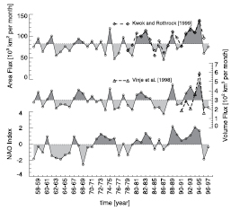
Figure 4.12. Time series of modelled Fram Strait sea ice area and volume flux, along with the NAO index. Also shown are observational estimates of area flux ( Kwok and Rothrock, 1999 [JoC, SRC] ) and volume flux ( Vinje et al., 1998 [JoC] ). Reproduced from Hilmer and Jung 2000 [JoC] ).
4.5 Changes in Glaciers and Ice Caps
4.5.1 Background
Those glaciers and ice caps not immediately adjacent to the large ice sheets of Greenland and Antarctica cover an area between 512 × 103 and 546 × 103 km2 according to inventories from different authors( Table 4.3 ); volume estimates differ considerably from 51 × 103 to 133 × 103 km3,representing sea level equivalent (SLE) of between 0.15 and 0.37 m. Including the glaciers and ice caps surrounding the Greenland Ice Sheet and West Antarctica, but excluding those on the Antarctic Peninsula and those surrounding East Antarctica, yields 0.72 ± 0.2 m SLE. These new estimates are about 40% higher than those given in IPCC 2001 [NPR] ), but area inventories are still incomplete and volume measurements more so, despite increasing efforts.
Table 4.3. Extents of glaciers and ice caps as given by different authors.
| Reference | Area (103 km2) | Volume (103 km3) | SLEf (m) |
|---|---|---|---|
| Raper and Braithwaite, 2005a,c | 522 ± 42 | 87 ± 10 | 0.24 ± 0.03 |
| Ohmura, 2004a,d | 512 | 51 | 0.15 |
| Dyurgerov and Meier, 2005a,e | 546 ± 30 | 133 ± 20 | 0.37 ± 0.06 |
| Dyurgerov and Meier, 2005b,e | 785 ± 100 | 260 ± 65 | 0.72 ± 0.2 |
| IPCC, 2001b | 680 | 180 ± 40 | 0.50 ± 0.1 |
Glaciers and ice caps provide among the most visible indications of the effects of climate change. The mass balance at the surface of a glacier (the gain or loss of snow and ice over a hydrological cycle) is determined by the climate. At high and mid-latitudes, the hydrological cycle is determined by the annual cycle of air temperature, with accumulation dominating in winter and ablation in summer. In wide parts of the Himalaya most accumulation and ablation occur during summer ( Fujita and Ageta, 2000 [MoS] ), in the tropics ablation occurs year round and the seasonality in precipitation controls accumulation ( Kaser and Osmaston, 2002 [NPR, SRC] ). A climate change will affect the magnitude of the accumulation and ablation terms and the length of the mass balance seasons. The glacier will then change its extent towards a size that makes the total mass balance (the mass gain or loss over the entire glacier) zero. However, climate variability and the time lag of the glacier response mean that static equilibrium is never attained. Changes in glacier extent lag behind climate changes by only a few years on the short, steep and shallow glaciers of the tropical mountains with year-round ablation ( Kaser et al., 2003 [SRC] ), but by up to several centuries on the largest glaciers and ice caps with small slopes and cold ice ( Paterson, 2004 [NPR] ). Glaciers also lose mass by iceberg calving: this does not have an immediate and straightforward link to climate, but general relations to climate can often be discerned. Mass loss by basal melting is considered negligible at a global or large regional scale.
4.5.2 Large and Global-Scale Analyses
Records of glacier length changes (WGMS(ICSI-IAHS), various years-a) go far back in time – written reports as far back as 1600 in a few cases – and are directly related to low-frequency climate change. From 169 glacier length records, Oerlemans 2005 [JoC, ARC] ) compiled mean length variations of glacier tongues for large-scale regions between 1700 and 2000 ( Figure 4.13 ). Although much local, regional and high-frequency variability is superimposed, the smoothed series give an apparently homogeneous signal. General retreat of glacier tongues started after 1800, with considerable mean retreat rates in all regions after 1850 lasting throughout the 20th century. A slow down of retreat between about 1970 and 1990 is more evident in the raw data ( Oerlemans, 2005 [JoC, ARC] ). Retreat was again generally rapid in the 1990 s; the Atlantic and the SH curves reflect precipitation-driven growth and advances of glaciers in western Scandinavia and New Zealand during the late 1990 s ( (Chinn et al., 2005 ) ).
Records of directly measured glacier mass balances are few and stretch back only to the mid-20th century. Because of the very intensive fieldwork required, these records are biased towards logistically and morphologically ‘easy’ glaciers. Uncertainty in directly measured annual mass balance is typically ±200 kgm–2 yr–1 due to measurement and analysis errors ( Cogley, 2005 [NPR, SRC] ). Mass balance data are archived and distributed by the World Glacier Monitoring Service (WGMS(ICSI-IAHS), various years-b). From these and from several other new and historical sources, quality checked time series of the annual mean specific mass balance (the total mass balance of a glacier or ice cap divided by its total surface area) for about 300 individual glaciers have been constructed, analysed and presented in three databases ( Ohmura, 2004 [NPR, SRC] ; Cogley, 2005 [NPR, SRC] ; Dyurgerov and Meier, 2005 [NPR, SRC] Dyurgerov and Meier 2005 [NPR, SRC] ) also incorporated recent findings from repeat altimetry of glaciers and ice caps in Alaska ( Arendt et al., 2002 [JoC] ) and Patagonia ( Rignot et al., 2003 [JoC, SRC] ). Only a few individual series stretch over the entire period. From these statistically small samples, global estimates have been obtained as five-year (pentadal) means by arithmetic averaging (C05a in Figure 4.14 ), area-weighted averaging (DM05 and O04) and spatial interpolation (C05i). Although mass balances reported from individual glaciers include the effect of changing glacier area, deficiencies in the inventories do not allow for general consideration of area changes. The effect of this inaccuracy is considered minor. Table 4.4 summarises the data plotted in Figure 4.14 .
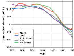
Figure 4.13. Large-scale regional mean length variations of glacier tongues ( Oerlemans, 2005 [JoC, ARC] ). The raw data are all constrained to pass through zero in 1950 . The curves shown are smoothed with the ( Stineman 1980 ) ) method and approximate this. Glaciers are grouped into the following regional classes: SH (tropics, New Zealand, Patagonia), northwest North America (mainly Canadian Rockies), Atlantic (South Greenland, Iceland, Jan Mayen, Svalbard, Scandinavia), European Alps and Asia (Caucasus and central Asia).
Table 4.4. Global average mass balance of glaciers and ice caps for different periods, showing mean specific mass balance (kgm–2 yr–1); total mass balance (Gt yr–1); and SLE (mm yr–1)derived from total mass balance and an ocean surface area of 362 × 106 km2.Values for glaciers and ice caps excluding those around the ice sheets (total area 546 × 103 km2)are derived from MB values in Figure 4.14 .Values for glaciers and ice caps including those surrounding Greenland and West Antarctica (total area 785.0 × 10³ km2)are modified from Dyurgerov and Meier 2005 [NPR, SRC] ) by applying pentadal DM05 to MB ratios. Uncertainties are for the 90% confidence level. Sources: Ohmura 2004 [NPR, SRC] Cogley 2005 [NPR, SRC] and Dyurgerov and Meier 2005 [NPR, SRC] ), all updated to 2003 / 2004 .
| Period | Mean Specific Mass Balancea (kgm–2 yr–1) | Total Mass Balancea (Gt yr–1) | Sea Level Equivalenta (mm yr–1) | Mean Specific Mass Balanceb (kgm–2 yr–1) | Total Mass Balanceb (Gt yr–1) | Sea LevelEquivalentb (mm yr–1) |
|---|---|---|---|---|---|---|
|
1960/1961–2003/2004 |
–283 ± 102 | –155 ± 55 | 0.43 ± 0.15 | –231 ± 82 | –182 ± 64 | 0.50 ± 0.18 |
|
1960/1961–1989/1990 |
–219 ± 92 | –120 ± 50 | 0.33 ± 0.14 | –173 ± 73 | –136 ± 57 | 0.37 ± 0.16 |
|
1990/1991–2003/2004 |
–420 ± 121 | –230 ± 66 | 0.63 ± 0.18 | –356 ± 101 | –280 ± 79 | 0.77 ± 0.22 |
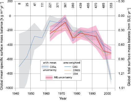
Figure 4.14. Pentadal (five-year) average mass balance of the world’s glaciers and ice caps excluding those around the ice sheets of Greenland and Antarctica. Mean specific mass balance (left axis) is converted to total mass balance and to SLE (right axis) using the total ice surface area of 546 × 103 km2 ( Table 4.3 )and the ocean surface area of 362 × 106 km2.C05a is an arithmetic mean over all annual measurements within each pentade ( Cogley, 2005 [NPR, SRC] ); the grey envelope is the 90% confidence level of the C05a data and represents the spatial variability of the measured mass balances. The number of measurements in each time period is given at the top of the graph. C05i is obtained by spatial interpolation ( Cogley, 2005 [NPR, SRC] ), while DM05 ( Dyurgerov and Meier, 2005 [NPR, SRC] ) and O04 ( Ohmura, 2004 [NPR, SRC] ) are area-weighted global numbers. MB is the arithmetic mean of C05i, DM05 and O04, and its uncertainty (red shading) combines the spatial variability and the structural uncertainty calculated for the 90% confidence level. This does not include uncertainties that derive from uncertainties in the glacier area inventories. The authors performed area weighting and spatial interpolation only after 1960, when up to 100 measured mass balances were available. The most recent period consists of four years only ( 2000 / 2001 to 2003 / 2004 ).
The time series of globally averaged mean specific mass balance from different authors have very similar shapes despite some offsets in magnitude. Around 1970, mass balances were close to zero or slightly positive in most regions( Figure 4.15 )and close to zero in the global mean( Figure 4.14 ), indicating near-equilibration with climate after the strong earlier mass loss. This gives confidence that the glacier wastage in the late 20th century is essentially a response to post- 1970 global warming ( (Greene, 2005 ) ). Strong mass losses are indicated for the 1940 s but uncertainty is great since the arithmetic mean values (C05a in Figure 4.14 )are from only a few glaciers. The most recent period consists of four years only ( 2000 / 2001 – 2003 / 2004 ) and does not cover all regions completely. The shortage of data from Alaska and Patagonia likely causes a positive bias on the area-weighted and interpolated analyses (DM05, O04, C05i) due to the large ice areas in these regions. There is probably also a negative bias in the arithmetic mean (C05a), due to the strongly negative northern mid-latitudes mass balances in 2002 / 2003, particularly in the European Alps ( Zemp et al., 2005 [NPR, SRC] ). Mass loss rates for 1990 / 1991 to 2003 / 2004 are roughly double those for 1960 / 1961 to 1989 / 1990 ( Table 4.4 ).
Over the last half century, both global mean winter accumulation and summer melting have increased steadily ( Ohmura, 2004 [NPR, SRC] ; Dyurgerov and Meier, 2005 [NPR, SRC] ;( Greene, 2005 ) ). At least in the NH, winter accumulation and summer melting correlate positively with hemispheric air temperature, whereas the mean specific mass balance correlates negatively with hemispheric air temperature ( (Greene, 2005 ) Dyurgerov and Dwyer 2000 [SRC] ) analysed time series of 21 NH glaciers and found a rather uniformly increased mass turnover rate, qualitatively consistent with moderately increased precipitation and substantially increased low-altitude melting. This general trend is also indicated for Alaska ( Arendt et al., 2002 [JoC] ), the Canadian Arctic Archipelago ( Abdalati et al., 2004 [JoC] ) and Patagonia ( Rignot et al., 2003 [JoC, SRC] ).
Regional analyses by Dyurgerov and Meier 2005 [NPR, SRC] ) show strongest negative mean specific mass balances in Patagonia, the northwest USA and southwest Canada, and Alaska, with losses especially rapid in Patagonia and Alaska after the mid- 1990 s( Figure 4.15 a). A cumulative mean specific mass balance of –10 × 103 kgm–2 corresponds to a loss of 10 m of water, or about 11 m of ice, averaged over the glacier area; cumulative losses in Patagonia since 1960 are approximately 40 m of ice thickness averaged over the glaciers. Only Europe showed a mean value close to zero, with strong mass losses in the Alps compensated by mass gains in maritime Scandinavia until the end of the 20th century. High spatial variability in climate and, thus, in glacier variations, also exists in other large regions such as in the high mountains of Asia ( Liu et al., 2004 [SRC] ; Dyurgerov and Meier, 2005 [NPR, SRC] ). Values for Patagonia and Alaska are mainly derived from altimetry evaluations made by Arendt et al. 2002 [JoC] and Rignot et al. 2003 [JoC, SRC] ), and authors of both papers note that the observed mass losses cannot be explained by surface mass loss only, but also include increased ice discharge due to enhanced ice velocity. The latter, in turn, has possibly been triggered by previous negative mass balances of glaciers calving icebergs, as well as by increased melt water production that enhances basal sliding. Some glaciers exhibit quasi-periodic internal instabilities (surging), which can affect data from those glaciers ( Arendt et al., 2002 [JoC] ; Rignot et al., 2003 [JoC, SRC] ), but these effects are expected to average very close to zero over large regions and many years or decades. Because of a lack of suitable information, the temporal variation of the mass loss of the Patagonian ice fields has been interpolated to match the time series of Alaskan mass balances assuming similar climate regimes ( Dyurgerov and Meier, 2005 [NPR, SRC] ).
The surface mass balance of snow and ice is determined by a complex interaction of energy fluxes towards and away from the surface and the occurrence of solid precipitation. Nevertheless, glacier fluctuations show a strong statistical correlation with air temperature at least at a large spatial scale throughout the 20th century ( (Greene, 2005 ) ), and a strong physical basis exists to explain why warming would cause mass loss ( Ohmura, 2001 [JoC, SRC] ). Changes in snow accumulation also matter, and may dominate in response to strong circulation changes or when temperature is not changing greatly. For example, analyses of glacier mass balances, volume changes, length variations and homogenised temperature records for the western portion of the European Alps ( Vincent et al., 2005 [JoC] ) clearly indicate the role of precipitation changes in glacier variations in the 18th and 19th centuries. Similarly, Nesje and Dahl 2003 [JoC] ) explained glacier advances in southern Norway in the early 18th century as being due to increased winter precipitation rather than colder temperatures.
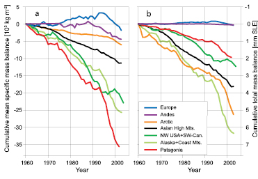
Figure 4.15. Cumulative mean specific mass balances (a) and cumulative total mass balances (b) of glaciers and ice caps, calculated for large regions ( Dyurgerov and Meier, 2005 [NPR, SRC] ). Mean specific mass balance shows the strength of climate change in the respective region. Total mass balance is the contribution from each region to sea level rise.
Total mass balances are the integration of mean specific mass balances (which have a climate signal) over the existing glacier area. Consequently, the biggest mass losses and, thus, contributions to sea level rise are from Alaska with 0.11 mm yr–1 SLE from 1960 / 1961 to 1989 / 1990 and 0.24 mm yr–1 SLE from 1990 / 1991 to 2002 / 2003, the Arctic (0.09 and 0.19), and the high mountains of Asia (0.08 and 0.10)( Figure 4.15 b).
4.5.3 Special Regional Features
Although reports on individual glaciers or limited glacier areas support the global picture of ongoing strong ice shrinkage in almost all regions, some exceptional results indicate the complexity of both regional- to local-scale climate and respective glacier regimes.
For glaciers in the dry and cold Taylor Valley, Antarctica, ( Fountain et al. 2004 ) ) hypothesised that an increase in average air temperature of 2°C alone can explain the observed glacier advance through ice softening.
Altimetric measurements in Svalbard suggested a small ice cap growth ( Bamber et al., 2004 [JoC] ), however, an alternative evaluation of mass balance processes indicates a slight sea level contribution of 0.01 mm yr–1 for the last three decades of the 20th century ( Hagen et al., 2003 [SRC] ). Svalbard glaciers were recently close to balance, which is exceptional for the Arctic.
In Scandinavia, Norwegian coastal glaciers, which advanced in the 1990 s due to increased accumulation in response to a positive phase of the NAO ( (Nesje et al., 2000 ) ), started to shrink around 2000 as a result of a combination of reduced winter accumulation and greater summer melting ( Kjøllmoen, 2005 [NPR] ). Norwegian glacier tongues farther inland have retreated continuously at a moderate rate. Warming is also indicated by a change in temperature distribution in northern Sweden’s Storglaciären where, between 1989 and 2001, 8.3 m of the cold surface layer (or 22% of the long-term average thickness of this cold layer) warmed to the melting point. This is attributed primarily to increased winter temperatures yielding a longer melt season; summer ablation was normal ( Pettersson et al., 2003 [JoC, SRC] ). As with coastal Scandinavia, glaciers in the New Zealand Alps advanced during the 1990 s, but have started to shrink since 2000 . Increased precipitation may have caused the glacier growth ( (Chinn et al., 2005 ) ).
In the European Alps, exceptional mass loss during 2003 removed an average of 2,500 kgm–2 yr–1 over nine measured Alpine glaciers, almost 60% higher than the previous record of 1,600 kgm–2 yr–1 loss in 1996 and four times more than the mean loss from 1980 to 2001 (600 kgm–2 yr–1 ;Zemp et al., 2005 [NPR, SRC] ). This was caused by extraordinarily high air temperatures over a long period, extremely low precipitation, and albedo feedback from Sahara dust depositions and a previous series of negative mass balance years (see Box 3.6 .).
Whereas glaciers in the Asian high mountains have generally shrunk at varying rates ( (Su and Shi, 2002; ) Ren et al., 2004 [SRC] ; Solomina et al., 2004 [MoS, SRC] ; Dyurgerov and Meier, 2005 [NPR, SRC] ), several high glaciers in the central Karakoram are reported to have advanced and/or thickened at their tongues ( (Hewitt, 2005 ) ), probably due to enhanced precipitation.
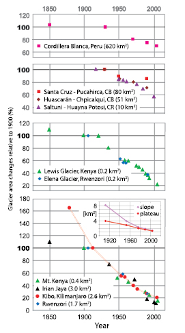
Figure 4.16. Changes in the surface area of tropical glaciers relative to their extent around 1900, grouped according to different glacier sizes. The sizes are given for 1990 or the closest available date to 1990 . The broken red line highlights the retreat of Kilimanjaro glaciers. The insert shows the area change (km2)of the Kilimanjaro plateau (red) and slope (purple) glaciers as separated by the 5,700 m contour line ( Kaser and Osmaston, 2002 [NPR, SRC] (updated courtesy of S. Lieb); Mölg et al., 2003b [JoC, MoS, SRC] ;( Georges, 2004; ) ( Hastenrath, 2005; ) Cullen et al., 2006 [JoC] ;( Klein and Kincaid, 2006 ) ).
Tropical glaciers have shrunk from a maximum in the mid-19th century, following the global trend( Figure 4.16 ). Strong shrinkage rates in the 1940 s were followed by relatively stable extents that lasted into the 1970 s. Since then, shrinkage has become stronger again; as in other mountain ranges, the smallest glaciers are more strongly affected. Since the publication of IPCC 2001 [NPR] ), evidence has increased that changes in the mass balance of tropical glaciers are mainly driven by coupled changes in energy and mass fluxes related to interannual variations of regional-scale hygric seasonality ( (Wagnon et al., 2001; ) Francou et al., 2003 [JoC] , 2004 ). Variations in atmospheric moisture content affect incoming solar radiation, precipitation and albedo, atmospheric longwave emission, and sublimation ( (Wagnon et al., 2001; ) Kaser and Osmaston, 2002 [NPR, SRC] ; Mölg et al., 2003a [JoC, SRC] ; Favier et al., 2004 [JoC, MoS] ; Mölg and Hardy, 2004 [JoC] ; Sicart et al., 2005 [JoC] ). At a large scale, the mass balance of tropical glaciers strongly correlates with tropical sea surface temperature anomalies and related atmospheric circulation modes ( Francou et al., 2003 [JoC] , 2004; Favier et al., 2004 [JoC, MoS] ). Glaciers on Kilimanjaro behaved exceptionally throughout the 20th century( Figure 4.16 ). The geometry of the volcano and the dry climate above the freezing level maintain vertical ice walls around the tabular ice on the summit plateau and these retreat at about 0.9 m yr–1 ( Thompson et al., 2002 [JoC, ARC] ) forced by solar radiation ( Mölg et al., 2003b [JoC, MoS, SRC] ). Their retreat is responsible for the steady shrinkage of the ice area on the summit plateau( Figure 4.16 ,insert) ( Cullen et al., 2006 [JoC] ). In contrast, the slope glaciers, which extend from the plateau rim onto the steep slopes of the volcano, decreased strongly at the beginning of the 20th century, but more slowly recently. This shrinkage is interpreted as an ongoing response to a dramatic change from a wetter to a drier regime, supposedly around 1880, and a subsequent negative trend in mid-troposphere atmospheric moisture content over East Africa ( Cullen et al., 2006 [JoC] ).
4.6 Changes and Stability of Ice Sheets and Ice Shelves
New and improved observational techniques, and extended time series, reveal changes in many parts of the large ice sheets. Greenland has experienced mass loss recently in response to increases in near-coastal melting and in ice flow velocity more than offsetting increases in snowfall. Antarctica appears to be losing mass at least partly in response to recent ice flow acceleration in some near-coastal regions, although with greater uncertainty in overall balance than for Greenland. Shortcomings in forcing, physics and resolution in comprehensive ice flow models have prevented them from fully capturing the ice flow changes.
4.6.1 Background
The ice sheets of Greenland and Antarctica hold enough ice to raise sea level about 64 m if fully melted ( Bamber et al., 2001 [JoC] ; Lythe et al., 2001 [JoC, MoS, SRC] ). Even a modest change in ice sheet balance could strongly affect future sea level and freshwater flux to the oceans, with possible climatic implications. These ice sheets consist of vast central reservoirs of slow-moving ice drained by rapidly moving, ice-walled ice streams or rock-walled outlet glaciers typically flowing into floating ice shelves or narrower ice tongues, or directly into the ocean. Ice shelves often form in embayments, or run aground on local bedrock highs to produce ice rumples or ice rises, and friction with embayment sides or local grounding points helps restrain the motion of the ice shelves and their tributaries. About half of the ice lost from Greenland is by surface melting and runoff into the sea, but surface melting is much less important to the mass balance of Antarctica. Dynamics of the slow-moving ice and of ice shelves are reasonably well understood and can be modelled adequately, but this is not so for fast-moving ice streams and outlet glaciers. Until recently (including IPCC, 2001 [NPR] ), it was assumed that velocities of these outlet glaciers and ice streams cannot change rapidly, and impacts of climate change were estimated primarily as changes in snowfall and surface melting. Recent observations show that outlet glacier and ice stream speeds can change rapidly, for reasons that are still under investigation. Consequently, this assessment will not adequately quantify such effects.
4.6.2 Mass Balance of the Ice Sheets and Ice Shelves
The current state of balance of the Greenland and Antarctic Ice Sheets is discussed here, focussing on the substantial progress made since IPCC 2001 [NPR] ). Possible future changes are considered in Chapter 10 ,and in Chapter 19 of the Working Group II contribution to the IPCC Fourth Assessment Report.
4.6.2.1 Techniques
Several techniques are used to measure the mass balance of large ice masses. The mass budget approach compares input from snow accumulation with output from ice flow and melt water runoff. Repeated altimetry measures surface elevation changes. Temporal variations in gravity over the ice sheets reveal mass changes. Changes in day length and in the direction of the Earth’s rotation axis also reveal mass redistribution.
4.6.2.1.1 Mass budget
Snow accumulation is often estimated from annual layering in ice cores, with interpolation between core sites using satellite microwave measurements or radar sounding ( Jacka et al., 2004 [JoC] ). Increasingly, atmospheric modelling techniques are also applied (e.g., Monaghan et al., 2006 [JoC] ). Ice discharge is calculated from radar or seismic measurements of ice thickness, and from in situ or remote measurements of ice velocity, usually where the ice begins to float and velocity is nearly depth-independent. A major advance since IPCC 2001 [NPR] ) has been widespread application of Interferometric Synthetic Aperture Radar (InSAR) techniques from satellites to measure ice velocity over very large areas of the ice sheets (e.g., Rignot et al., 2005 [JoC, SRC] ). Calculation of mass discharge also requires estimates for runoff of surface melt water, which is large for low-elevation regions of Greenland and parts of the Antarctic Peninsula but small or zero elsewhere on the ice sheets. Surface melt amounts usually are estimated from modelling driven by atmospheric reanalyses, global models or climatology, and often calibrated against surface observations where available (e.g., Hanna et al., 2005 [JoC] ; Box et al., 2006 [JoC, SRC] ). The typically small mass loss by melting beneath grounded ice is usually estimated from models. Mass loss from melting beneath ice shelves can be large, and is difficult to measure; it is generally calculated as the remainder after accounting for other mass inputs and outputs.
Ice sheet mass inputs and outputs are difficult to estimate with high accuracy. For example, van de Berg et al. 2006 [JoC, MoS] ) summarised six estimates of net accumulation on the grounded section of Antarctica published between 1999 and 2006, which ranged from 1,811 to 2,076 Gt yr–1 or ±7% about the midpoint. Transfer of 360 Gt of grounded (non-floating) ice to the ocean would raise sea level about 1 mm. Uncertainty in the Greenland accumulation rate is probably about 5% ( Hanna et al., 2005 [JoC] ; Box et al., 2006 [JoC, SRC] ). Although broad InSAR coverage and progressively improving estimates of grounding-line ice thickness have substantially improved ice discharge estimates, incomplete data coverage implies uncertainties in discharge estimates of a few percent. Uncorrelated errors of 5% on input and output would imply mass budget uncertainties of about 40 Gt yr–1 for Greenland and 140 Gt yr–1 for Antarctica. Large interannual variability and trends also complicate interpretation. Box et al. 2006 [JoC, SRC] ) estimated average accumulation on the Greenland Ice Sheet of 543 Gt yr–1 from 1988 to 2004, but with an annual minimum of 482 Gt yr–1,a maximum of 613 Gt yr–1 and a best-fit linear trend yielding an increase of 68 Gt yr–1 during the period. Glacier velocities can change substantially, sometimes in months or years, adding to the overall uncertainty of mass budget calculations.
4.6.2.1.2 Repeated altimetry
Surface elevation changes reveal ice sheet mass changes after correction for changes in depth-density profiles and in bedrock elevation, or for hydrostatic equilibrium if the ice is floating. Satellite radar altimetry (SRALT) has been widely used to estimate elevation changes ( Shepherd et al., 2002 [JoC, ARC] ; Davis et al., 2005 [JoC] ; Johannessen et al., 2005 [JoC] ;( Zwally et al., 2006 ) ), together with laser altimetry from airplanes ( Krabill et al., 2004 [JoC] ) and from the Ice, Cloud and land Elevation Satellite (ICESat; Thomas et al., 2006 [JoC, SRC] ). Modelled corrections for isostatic changes in bedrock elevation are small (a few millimetres per year), but with uncertainties nearly as large as the corrections in some cases ( (Zwally et al., 2006 ) ). Corrections for near-surface firn density changes are larger (>10 mm yr–1( ;Cuffey, 2001 ) ) and also uncertain.
Radar altimetry has provided long-term and widespread coverage for more than a decade, but with important challenges (described by Legresy et al., 2006 [NPR] ). The available SRALT data are from altimeters with a beam width of 20 km or more, designed and demonstrated to make accurate measurements over the almost flat, horizontal ocean. Data interpretation is more complex over sloping, undulating ice sheet surfaces with spatially and temporally varying dielectric properties and thus penetration into near-surface firn. Empirical corrections are applied for some of these effects, and for inter-satellite biases. The correction for the offset between the European Remote Sensing Satellite (ERS-1 and ERS-2) altimeters is reported by ( Zwally et al. 2006 ) ) to affect mass change estimates for the interval 1992 to 2002 by about 50 Gt yr–1 for Greenland, and to differ from the corresponding correction of Johannessen et al. 2005 [JoC] ) by about 20 Gt yr–1,although some of this difference may reflect differences in spatial coverage of the studies combined with spatial dependence of the correction. Changes in surface dielectric properties affect the returned waveform and thus the measured range, so a correction is made for elevation changes correlated to returned-power changes. This effect is small averaged over an ice sheet but often of the same magnitude as the remaining signal at a point, and could remove part or all of the signal if climate change affected both elevation and surface character, hence returned power.
The SRALT tracking algorithms use leading edges of reflected radar waveforms, thus primarily sampling higher-elevation parts of the large footprint. This probably introduces only small errors over most of an ice sheet, where surfaces are nearly flat. However, glaciers and ice streams often flow in surface depressions that can be narrower than the radar footprint, so that SRALT-derived elevation changes are weighted towards slower-moving ice at the glacier sides ( Thomas et al., 2006 [JoC, SRC] ). This is of most concern in Greenland, where other studies show thinning along outlet glaciers just a few kilometres wide ( Abdalati et al., 2001 [JoC] ). Elevation-change estimates from SRALT have not been validated against independent data except at higher elevations, where surfaces are nearly flat and horizontal and dielectric properties nearly unchanging ( Thomas et al., 2001 [JoC, SRC] ). Although SRALT coverage is lacking within 900 km of the poles, and some data are lost in steep regions, coverage has now been achieved for about 90% of the Greenland Ice Sheet and 80% of the Antarctic Ice Sheet ( (Zwally et al., 2006 ) )( Figure 4.19 ).
Laser altimeters reduce some of the difficulties with SRALT by having negligible penetration of near-surface layers and a smaller footprint (about 1 m for airborne laser, and 60 m for ICESat). However, clouds limit data acquisition, and accuracy is affected by atmospheric conditions and particularly by laser pointing errors. Airborne surveys over Greenland in 1993 / 1994 and 1998 / 1999 yielded estimates of elevation change accurate to ±14 mm yr–1 along survey tracks ( (Krabill et al., 2002 ) ). However, the large gaps between flight lines must be filled, often by simple interpolation in regions of weak variability or by interpolation using physical models in more complex regions ( Krabill et al., 2004 [JoC] ; Figure 4.17 ).
4.6.2.1.3 Geodetic measurements, including measurement of temporal variations in Earth gravity
Since 2002, the Gravity Recovery and Climate Experiment (GRACE) satellite mission has been providing routine measurement of the Earth’s gravity field and its temporal variability. After removing the effects of tides, atmospheric loading, etc., high-latitude data contain information on temporal changes in the mass distribution of the ice sheets and underlying rock ( Velicogna and Wahr, 2005 [JoC] ). Estimates of ice sheet mass balance are sensitive to modelled estimates of bedrock vertical motion, primarily arising from response to changes in mass loading from the end of the last ice age. Velicogna and Wahr 2005 [JoC] ) estimated a correction for Greenland Ice Sheet mass balance of 5 ± 17 Gt yr–1 for the bedrock motion, with an equivalent value of 177 ± 73 Gt yr–1 for Antarctica ( Velicogna and Wahr, 2006 [JoC] ). (Note that stated uncertainties for ice sheet mass balances referenced to published papers are given here as published. Some papers include error terms that were estimated without formal statistical derivations, and other papers note omission of estimates for certain possible systematic errors, so that these as-published errors generally cannot be interpreted as representing any specific confidence interval such as 5 to 95%.)
Other geodetic data provide constraints on mass changes at high latitudes. These data include the history of changing length of day from eclipse records, the related ongoing changes in the spherical-harmonic coefficients of the geopotential, and true polar wander (changes in the planet’s rotation vector; Peltier, 1998 [JoC] ; Munk, 2002 [JoC] ;( Mitrovica et al., 2006 ) ). At present, unique solutions are not possible from these techniques, but hypothesised histories of ice sheet changes can be tested against the data for consistency, and progress is rapidly being made.
4.6.2.2 Measured Balance of the Ice Sheets and Ice Shelves
Mass balance of the large ice sheets was summarised by Rignot and Thomas 2002 [JoC, SRC] and Alley et al. 2005a [JoC, SRC] ).
4.6.2.2.1 Greenland
Many recent studies have addressed Greenland mass balance. They yield a broad picture( Figure 4.17 )of inland thickening ( Thomas et al., 2001 [JoC, SRC] ; Johannessen et al., 2005 [JoC] ; Thomas et al., 2006 [JoC, SRC] ;( Zwally et al., 2006 ) ), faster near-coastal thinning primarily in the south along fast-moving outlet glaciers ( Abdalati et al., 2001 [JoC] ; Rignot and Kanagaratnam, 2006 [JoC, SRC] ), and a recent acceleration in overall shrinkage.
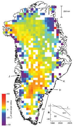
Figure 4.17. Rates of surface elevation change (dS/dt) derived from laser altimeter measurements at more than 16,000 locations on the Greenland Ice Sheet where ICESat data from 2005 overlay aircraft surveys in 1998 / 1999 (using methods described by Thomas et al., 2006 [JoC, SRC] ). Locations of rapidly thinning outlet glaciers at Jakobshavn (J), Kangerdlugssuaq (K), Helheim (H) and along the southeast coast (SE) are shown, together with an inset showing their estimated total mass balance (M∙ , Gt yr–1)between 1996 and 2005 ( Rignot and Kanagaratnam, 2006 [JoC, SRC] ).
Analysis of GRACE data showed total losses of 75 ± 26 Gt yr–1 between April 2002 and July 2004 ( Velicogna and Wahr, 2005 [JoC] Ramillien et al. 2006 [JoC] ), also working from GRACE data, found a mass loss of 129 ± 15 Gt yr–1 for July 2002 to March 2005 . Because of the low spatial resolution of GRACE, these include losses from isolated mountain glaciers and ice caps near the coast, whereas the results discussed next do not.
Mass loss from the ice sheet surface (net snow accumulation minus melt water runoff) has increased recently. Box et al. 2006 [JoC, SRC] ) used calibrated atmospheric modelling and a single approximation for ice flow discharge to estimate average ice sheet mass loss of more than 100 Gt yr–1 during 1988 to 2004; they also found acceleration of surface mass loss during this interval of 43 Gt yr–1.A similar analysis by Hanna et al. 2005 [JoC] ) for 1961 to 2003 found somewhat higher net accumulation but similar trends, with ice sheet growth of 22 ± 51 Gt yr–1 from 1961 to 1990, shifting to shrinkage of 14 ± 55 Gt yr–1 from 1993 to 1998 and shrinkage of 36 ± 59 Gt yr–1 from 1998 to 2003 . Again, ice flow acceleration was not included in these estimates.
In a study especially using SRALT but incorporating laser elevation measurements from aircraft and a correction for the effect of changing temperature on near-surface density, ( Zwally et al. 2006 ) ) estimated slight growth of the ice sheet by 11 ± 3 Gt yr–1 from 1992 to 2002 . However, they noted that mass loss of 18 ± 2 Gt yr–1 would be indicated if the thickness changes at higher elevations are largely low-density firn rather than high-density ice, as might apply if the effects of increasing accumulation rate were also taken into account ( Hanna et al., 2005 [JoC] ; Box et al., 2006 [JoC, SRC] ). The more spatially limited results of Johannessen et al. 2005 [JoC] ) from the same radar data indicated slightly less shrinkage or slightly more growth than found by ( Zwally et al. 2006 ) ) in regions of overlap. Krabill et al. 2000 [JoC] ) also found thickening of central regions (~10 mm yr–1)from laser measurements covering 1993 / 1994 to 1998 / 1999 .
Krabill et al. 2004 [JoC] ) used repeat laser altimetry and modelled surface mass balance to estimate mass loss of about 45 Gt yr–1 from 1993 / 1994 to 1998 / 1999, with acceleration to a loss of 73 ± 11 Gt yr–1 during the overlapping interval 1997 to 2003 . These values may underestimate total losses, because they do not take account of rapid thinning in sparsely surveyed regions such as the southeast, where mass budget studies show large losses ( Rignot and Kanagaratnam, 2006 [JoC, SRC] Thomas et al. 2006 [JoC, SRC] ) extended these results to 2004 using ICESat data to include approximate corrections for density changes in the near surface. Results showed ice sheet mass loss of 27 ± 23 Gt yr–1 for 1993 / 1994 to 1998 / 1999, loss of 55 ± 25 Gt yr–1 for 1997 to 2003, with an updated loss of 81 ± 24 Gt yr–1 from 1998 / 1999 to 2004 .
Rignot and Kanagaratnam 2006 [JoC, SRC] ) combined several data sets, with special focus on the acceleration in velocity of outlet glaciers measured by Synthetic Aperture Radar (SAR) interferometry. Starting from an estimated excess ice flow discharge of 51 ± 28 Gt yr–1 in 1996, these authors estimated that the ice flow loss increased to 83 ± 27 Gt yr–1 in 2000 and 150 ± 36 Gt yr–1 in 2005 . Adding surface mass balance deviations from the long-term average as calculated by Hanna et al. 2005 [JoC] ) yielded mass losses of 82 ± 28 Gt yr–1 in 1996, 124 ± 28 Gt yr–1 in 2000 and 202 ± 37 Gt yr–1 in 2005 . The more pronounced ice flow accelerations were restricted to regions south of 66°N before 2000 but extended to 70°N by 2005 . These estimates of rapid mass loss would be reduced somewhat if ice surface velocities are higher than depth-averaged velocities, which may apply in some places.
Greenland Ice Sheet mass balance estimates are summarised in Figure 4.18 (top). Most results indicate accelerating mass loss from Greenland during the 1990 s up to 2005 . The different estimates are not fully independent (there is, for example, some commonality in the isostatic corrections used for GRACE and altimetry estimates, and other overlaps can be found), but sufficient independence remains to increase confidence in the result. Different techniques have not fully converged quantitatively, with mismatches larger than formal error estimates suggesting structural uncertainties in the analyses, some of which were discussed above. The SRALT results showing overall near-balance or slight thickening, in contrast to other estimates, may result from the SRALT limitations over narrow glaciers discussed earlier.
Assessment of the data and techniques suggests a mass balance for the Greenland Ice Sheet ranging between growth of 25 Gt yr–1 and shrinkage of 60 Gt yr–1 for 1961 to 2003, shrinkage of 50 to 100 Gt yr–1 for 1993 to 2003 and shrinkage at even higher rates between 2003 and 2005 . Lack of agreement between techniques and the small number of estimates preclude assignment of statistically rigorous error bounds. Interannual variability is very large, driven mainly by variability in summer melting, but also by sudden glacier accelerations ( Rignot and Kanagaratnam, 2006 [JoC, SRC] ). Consequently, the short time interval covered by instrumental data is of concern in separating fluctuations from trends.
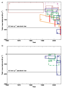
Figure 4.18. (Top) Mass balance estimates for Greenland. The coloured rectangles, following Thomas et al. 2006 [JoC, SRC] ), indicate the time span over which the measurements apply and the estimated range, given as (mean + uncertainty) and (mean – uncertainty) as reported in the original papers. Code: B (orange; Box et al, 2006 [JoC, SRC] ), surface mass balance, using stated trend in accumulation, ice flow discharge (assumed constant), and standard error on regression of accumulation trend, with added arrow indicating additional loss from ice flow acceleration; H (brown; Hanna et al., 2005 [JoC] ), surface mass balance, with arrow as for B; T (dark green; Thomas et al., 2006 [JoC, SRC] ), laser altimetry, showing new results and revision of Krabill et al. 2004 [JoC] ) to include firn densification changes; Z (violet; ( Zwally et al., 2006 ) ), primarily radar altimetry, with uncertainty reflecting the difference between a thickness change due to ice everywhere and that due to low-density firn in the accumulation zone; R (red; Rignot and Kanagaratnam, 2006 [JoC, SRC] ), ice discharge combined with surface mass balance; V (blue; Velicogna and Wahr, 2005 [JoC] ) GRACE gravity; RL (blue; Ramillen et al., 2006 ) GRACE gravity; J (magenta dashed; Johannessen et al., 2005 [JoC] ), radar altimetry without firn densification correction and applying only to central regions that are thickening but omitting thinning of coastal regions. (Bottom) Mass balance estimates for grounded ice of Antarctica. Coloured rectangles show age span and error range as in the top panel. Code: Z (violet; ( Zwally et al., 2006 ) ), radar altimetry, with uncertainty reflecting the difference between a thickness change due to ice everywhere and that due to low-density firn everywhere; RT (dark green; Rignot and Thomas, 2002 [JoC, SRC] ), ice discharge and surface mass balance, with dashed end line because some of the accumulation rate data extend beyond the time limits shown; RT2 (dark green; Rignot and Thomas, 2002 [JoC, SRC] ), updated to include additional mass losses indicated by Thomas et al. 2004 [Ambiguous] and Rignot et al. 2005 [JoC, SRC] ), dashed because the original authors did not produce this as an estimate for the whole ice sheet nor are accumulation rates updated; V (blue; Velicogna and Wahr, 2006 [JoC] ), GRACE gravity; RL (blue; Ramillen et al., 2006 ), GRACE gravity.
4.6.2.2.2 Antarctica
Recent estimates of Antarctic Ice Sheet mass balance are summarised in Figure 4.18 (bottom). Rignot and Thomas 2002 [JoC, SRC] ) combined several data sets including improved estimates of glacier velocities from InSAR to obtain antarctic mass budget estimates. For East Antarctica, growth of 20 ± 21 Gt yr–1 was indicated, with estimated losses of 44 ± 13 Gt yr–1 from West Antarctica. The balance of the Antarctic Peninsula was not assessed. Combining the East and West Antarctic numbers yielded a loss of 24 ± 25 Gt yr–1 for the region monitored. The time interval covered by these estimates is not tightly constrained, because ice input was estimated from data sets of varying length; output data were determined primarily in the few years before 2002 .
( Zwally et al. 2006 ) ) obtained SRALT coverage for about 80% of the ice sheet, including some portions of the Antarctic Peninsula, and interpolated to the rest of the ice sheet. The resulting balance included West Antarctic loss of 47 ± 4 Gt yr–1,East Antarctic gain of 17 ± 11 Gt yr–1 and overall loss of 30 ± 12 Gt yr–1.If all the ice thickness changes were low-density firn rather than ice, the loss would be smaller (14 ± 5 Gt yr–1 Davis et al. 2005 [JoC] ) compiled SRALT data for about 70% of the ice sheet, and did not interpolate to the rest. The same pattern of East Antarctic thickening and West Antarctic thinning was observed( Figure 4.19 Davis et al. 2005 [JoC] ) suggested that the East Antarctic change was primarily from increased snowfall. Assigning all thickness change to low-density firn produces growth of the monitored portions of the ice sheet of 45 ± 8 Gt yr–1;if all thickness changes were ice, this growth would be 105 ± 20 Gt yr–1.Following the suggestion that the East Antarctic changes are from increased snow accumulation and the West Antarctic changes are more likely to be ice-dynamical would yield growth of monitored regions of 33 ± 9 Gt yr–1.Note, however, that Monaghan et al. 2006 [JoC] ) did not find the strong increase in snow accumulation suggested by Davis et al. 2005 [JoC] ) in arguing for use of low-density firn in East Antarctic changes.
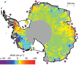
Figure 4.19. Rates of surface elevation change (dS/dt) derived from ERS radar-altimeter measurements between 1992 and 2003 over the Antarctic Ice Sheet ( Davis et al., 2005 [JoC] ). Locations of ice shelves estimated to be thickening or thinning by more than 30 cm yr–1( (Zwally et al., 2006 ) ) are shown by red triangles (thickening) and purple triangles (thinning).
Rignot et al. 2005 [JoC, SRC] ) documented discharges 84 ± 30% larger than accumulation rates for the glaciers that feed the Wordie Ice Shelf on the west coast of the northern Antarctic Peninsula (which shrank greatly between 1966 and 1989 ), a region largely absent from the SRALT studies. Consideration of strong imbalances in glaciers feeding the former Larsen B Ice Shelf across the Peninsula, and extrapolation of the results to undocumented basins, suggested mass loss from the ice in the northern part of the Antarctic Peninsula of 42 ± 7 Gt yr–1.Observation of widespread glacier front retreat in the region ( Cook et al., 2005 [JoC, SRC] ) motivates the extrapolation, although mass loss would be overestimated if snow accumulation has been systematically underestimated ( van de Berg et al., 2006 [JoC, MoS] ).
Taking the Rignot and Thomas 2002 [JoC, SRC] ( Zwally et al. 2006 ) and Rignot et al. 2005 [JoC, SRC] ) results as providing the most complete antarctic coverage suggests ice sheet thinning of about 60 Gt yr–1,with uncertainty of similar magnitude to the signal. Consideration of acceleration of some near-coastal glaciers, discussed below, and the difficulty of SRALT sampling of such regions, might allow slightly faster mass loss. The time interval considered is not uniform; the Rignot et al. 2005 [JoC, SRC] ) results include changes after the collapse of the Larsen B Ice Shelf in 2002, more recent than data in the other studies, and suggest the possibility of accelerating mass loss. Use of the more spatially restricted Davis et al. 2005 [JoC] ) SRALT data rather than the ( Zwally et al. 2006 ) ) results illustrates the persistent uncertainties; depending on the assumed density structure of the changes, Davis et al. 2005 [JoC] ) combined with the Rignot et al. 2005 [JoC, SRC] ) estimate for the Antarctic Peninsula would suggest near-balance or antarctic growth.
Interpretations of GRACE satellite gravity data indicate mass loss from the Antarctic Ice Sheet, including the Antarctic Peninsula and small glaciers and ice caps nearby, of 139 ± 73 Gt yr–1 between April 2002 and July 2005 ( Velicogna and Wahr, 2006 [JoC] ). Near-balance was indicated for East Antarctica, at 0 ± 51 Gt yr–1,with mass loss in West Antarctica of 136 ± 21 Gt yr–1.Independent analyses by Ramillien et al. 2006 [JoC] ) found, for July 2002 to March 2005, East Antarctic growth of 67 ± 28 Gt yr–1,West Antarctic shrinkage of 107 ± 23 Gt yr–1 and a net antarctic loss of 40 ± 36 Gt yr–1.
Assessment of the data and techniques suggests overall Antarctic Ice Sheet mass balance ranging from growth of 50 Gt yr–1 to shrinkage of 200 Gt yr–1 from 1993 to 2003 . As in the case of Greenland, the small number of measurements, lack of agreement between techniques, and existence of systematic errors that cannot be estimated accurately preclude formal error analyses and confidence limits. There is no implication that the midpoint of the range given provides the best estimate. Lack of older data complicates a similar estimate for the period 1961 to 2003 . Acceleration of mass loss is likely to have occurred, but not so dramatically as in Greenland. Considering the lack of estimated strong trends in accumulation rate, assessment of the possible acceleration and the slow time scales affecting central regions of the ice sheets, it is reasonable to estimate that the behaviour from 1961 to 2003 falls between ice sheet growth of 100 Gt yr–1 and shrinkage of 200 Gt yr–1.
Simply summing the 1993 to 2003 contributions from Greenland and Antarctica produces a range from balance (0 Gt yr–1)to shrinkage of 300 Gt yr–1,or a contribution to sea level rise of 0 to 0.8 mm yr–1.Because it is very unlikely that each of the ice sheets would exhibit the upper limit of its estimated mass balance range, it is very likely that, taken together, the ice sheets in Greenland and Antarctica have been contributing to sea level rise over the period 1993 to 2003 . For 1961 to 2003, the same calculation spans growth of 125 Gt yr–1 to shrinkage of 260 Gt yr–1,with 1993 to 2003 likely having the fastest mass loss of any decade in the 1961 to 2003 interval. Geodetic data on Earth rotation and polar wander provide additional insight ( Peltier, 1998 [JoC] ). Although Munk 2002 [JoC] ) suggested that the geodetic data did not allow much contribution to sea level rise from ice sheets, subsequent reassessment of the errors involved in some of the data sets and analyses allows an anomalous late 20th century sea level rise of up to about 1 mm yr–1 (360 Gt yr–1)from land ice ( (Mitrovica et al., 2006 ) ). Estimated mountain glacier contributions do not supply this, so a contribution from the polar ice sheets is consistent with the geodetic constraints, although little change in polar ice is also consistent.
4.6.2.2.3 Ice shelves
Changes in the mass of ice shelves, which are already floating, do not directly affect sea level, but ice shelf changes can affect flow of adjacent ice that is not floating, and thus affect sea level indirectly. Most ice shelves are in Antarctica, where they cover an area of about 1.5 × 10⁶ km2,or 11% of the entire ice sheet, and where nearly all ice streams and outlet glaciers flow into ice shelves. By contrast, Greenland ice shelves occupy only a few thousand square kilometres, and many are little more than floating glacier tongues. Mass loss by surface melt water runoff is not important for most ice shelf regions, which lose mass primarily by iceberg calving and basal melting, although basal freeze-on occurs in some regions.
Developments since IPCC 2001 [NPR] ) include improved velocity and thickness data to estimate fluxes, and interpretation of repeated SRALT surveys over ice shelves to infer thickening or thinning rates. Melting of up to tens of metres per year has been estimated beneath deeper ice near grounding lines ( Rignot and Jacobs, 2002 [JoC, SRC] ; Joughin and Padman, 2003 [JoC, SRC] ). Significant changes are observed on most ice shelves, with both positive and negative trends, and with faster changes on smaller shelves. Overall, ( Zwally et al. 2006 ) ) estimated mass loss from ice shelves fed by glaciers flowing from West Antarctica of 95 ± 11 Gt yr–1,and mass gain to ice shelves fed by glaciers flowing from East Antarctica of 142 ± 10 Gt yr–1.Rapid thinning of more than 1 m yr–1,and locally more than 5 m yr–1,was observed between 1992 and 2001 for many small ice shelves in the Amundsen Sea and along the Antarctic Peninsula. Thinning of about 1 m yr–1 ( Shepherd et al., 2003 [JoC, ARC] ;( Zwally et al., 2006 ) ) preceded the fragmentation of almost all (3,300 km2)of the Larsen B Ice Shelf along the Antarctic Peninsula in fewer than five weeks in early 2002 ( Scambos et al., 2003 [NPR] ).
Box 4.1: Ice Sheet Dynamics and Stability
The ice sheets of Antarctica and Greenland could raise sea level greatly. Central parts of these ice sheets have been observed to change only slowly, but near the coast rapid changes over quite large areas have been observed. In these areas, uncertainties about glacier basal conditions, ice deformation and interactions with the surrounding ocean seriously limit the ability to make accurate projections.
Ice sheets are thick, broad masses of ice formed mainly from compaction of snow ( Paterson, 2004 [NPR] ). They spread under their own weight, transferring mass towards their margins where it is lost primarily by runoff of surface melt water or by calving of icebergs into marginal seas or lakes. Water vapour fluxes (sublimation and condensation), and basal melting or freezing (especially beneath ice shelves) may also be important processes of mass gain and loss.
Ice sheets flow by internal deformation, basal sliding or a combination of both. Deformation in ice occurs through solid-state processes analogous to those involved in polycrystalline metals that are relatively close to their melting points. Deformation rates depend on the gravitational stress (which increases with ice thickness and with the slope of the upper surface), temperature, impurities, and size and orientation of the crystals (which in turn depend in part on the prior deformational history of the ice). While these characteristics are not completely known, model tuning allows slow ice flow by deformation to be simulated with reasonable accuracy.
For basal sliding to be an important component of the total motion, melt water or deformable wet sediment slurries at the base are required for lubrication. While the central regions of ice sheets (typically above 2,000 m elevation) seldom experience surface melting, the basal temperature may be raised to the melting point by heat conducted from the earth’s interior, delivered by melt water transport, or from the ‘friction’ of ice motion. Sliding velocities under a given gravitational stress can differ by orders of magnitude, depending on the presence or absence of unconsolidated sediment, the roughness of the substrate and the supply and distribution of water. Basal conditions are well characterised in few regions, introducing important uncertainties to the modelling of basal motion.
Ice flow is often channelled into fast-moving ice streams (which flow between slower-moving ice walls) or outlet glaciers (with rock walls). Enhanced flow in ice streams arises either from higher gravitational stress linked to thicker ice in bedrock troughs, or from increased basal lubrication.
Ice flowing into a marginal sea or lake may break off immediately to form icebergs, or may remain attached to the ice sheet to become a floating ice shelf. An ice shelf moves forward, spreading and thinning under its own weight, and fed by snowfall on its surface and ice input from the ice sheet. Friction at ice shelf sides and over local shoals slows the flow of the ice shelf and thus the discharge from the ice sheet. An ice shelf loses mass by calving icebergs from the front and by basal melting into the ocean cavity beneath. Estimates based on available data suggest a 1°C ocean warming could increase ice shelf basal melt by 10 m yr–1,but inadequate knowledge of the bathymetry and circulation in the largely inaccessible ice shelf cavities restricts the accuracy of such estimates.
Ice deformation is nonlinear, increasing approximately proportional to the cube of the applied stress. Moreover, an increase in any of the six independent applied stresses (three stretching stresses and three shear stresses) increases the deformation rate for all other stresses. For computational efficiency, most long simulations with comprehensive ice flow models use a simplified stress distribution, but recent changes in ice sheet margins and ice streams cannot be simulated accurately with these models, demonstrating a need for resolving the full stress configuration. Development of such models is still in its infancy, with few results yet available.
Ice sheets respond to environmental forcing over numerous time scales. A surface warming may take more than 10,000 years to penetrate to the bed and change temperatures there, while a crevasse filled with melt water might penetrate to the bed and affect the temperature locally within minutes. Ice velocity over most of an ice sheet changes slowly in response to changes in the ice sheet shape or surface temperature, but large velocity changes may occur rapidly on ice streams and outlet glaciers in response to changing basal conditions or changes in the ice shelves into which they flow.
The palaeo-record of previous ice ages indicates that ice sheets shrink in response to warming and grow in response to cooling. The data also indicate that shrinkage can be far faster than growth. Understanding of the processes suggests that this arises both because surface melting rates can be much larger than the highest snowfall rates, and because ice discharge may be accelerated by strong positive feedbacks Paterson,The palaeo-record of previous ice ages indicates that ice sheets shrink in response to warming and grow in response to cooling. The data also indicate that shrinkage can be far faster than growth. Understanding of the processes suggests that this arises both because surface melting rates can be much larger than the highest snowfall rates, and because ice discharge may be accelerated by strong positive feedbacks Paterson, P.U. Clark et al., 1999 [Ambiguous] ). Thawing of the bed, loss of restraint from ice shelves or changes in melt water supply and transmission can increase flow speed greatly. The faster flow may then generate additional lubrication from frictional heating and from erosion to produce wet sediment slurries. Surface lowering as the faster flow thins the ice will enhance surface melting, and will reduce basal friction where the thinner ice becomes afloat. Despite competition from stabilising feedbacks, warming-induced changes have led to rapid shrinkage and loss of ice sheets in the past, with possible implications for the future.
4.6.3 Causes of Changes
4.6.3.1 Changes in Snowfall and Surface Melting
For Greenland, modelling driven by reanalyses and calibrated against surface observations indicates recent increases in temperature, precipitation minus evaporation, surface melt water runoff and net mass loss from the surface of the ice sheet, as well as areal expansion of melting and reduction in albedo ( Hanna et al., 2005 [JoC] , 2006; Box et al., 2006 [JoC, SRC] ). High interannual variability means that many of the trends are not highly significant, but the trends are supported by the consistency between the various component data sets and results from different groups. Estimated net snowfall minus melt water runoff includes an increase in the Greenland contribution to sea level rise of 58 Gt yr–1 between the 1961 to 1990 and 1998 to 2003 intervals ( Hanna et al., 2005 [JoC] ), or of 43 Gt yr–1 from 1998 to 2004 ( Box et al., 2006 [JoC, SRC] ).
For Antarctica, the recent summaries by van de Berg et al. 2006 [JoC, MoS] van den Broeke et al. 2006 [JoC] and Monaghan et al. 2006 [JoC] ) have updated trends in accumulation rate. Contrary to some earlier work, these new studies found no continent-wide significant trends in accumulation over the interval 1980 to 2004 ( van de Berg et al., 2006 [JoC, MoS] ; van den Broeke et al., 2006 [JoC] ) or 1985 to 2001 ( Monaghan et al., 2006 [JoC] ) from atmospheric reanalysis products (National Centers for Environmental Prediction (NCEP), the European Centre for Medium Range Weather Forecasts (ECMWF), Japanese), or from two mesoscale models driven by ECMWF and one by NCEP reanalyses. Strong interannual variability was found, approaching 5% for the continent, and important regional and seasonal trends that fit into larger climatic patterns, including an upward trend in accumulation in the Antarctic Peninsula. Studies of surface temperature (e.g., van den Broeke, 2000 [JoC] ; Vaughan et al., 2001 [JoC, SRC] ; Thompson and Solomon, 2002 [PoC, JoC, ARC] ; Doran et al., 2002 [JoC] ; Schneider et al., 2004 [JoC, SRC] ; Turner et al., 2005 [JoC] ) similarly showed regional patterns including strong warming in the Antarctic Peninsula region, and cooling at some other stations. Long-term data are very sparse, precluding confident identification of continent-wide trends.
4.6.3.2 Ongoing Dynamic Ice Sheet Response to Past Forcing
Because some portions of ice sheets respond only slowly to climate changes (decades to thousands of years or longer), past forcing may be influencing ongoing changes( Box 4.1 ). Some geologic data support recent and perhaps ongoing antarctic mass loss (e.g., Stone et al., 2003 [JoC] ). A comprehensive attempt to discern such long-term trends contributing to recently measured imbalances was made by Huybrechts 2002 [JoC, SRC] and Huybrechts et al. 2004 [JoC, MoS, SRC] ). They found little long-term trend in volume of the Greenland Ice Sheet, but a trend in antarctic shrinkage of about 90 Gt yr–1,primarily because of retreat of the West Antarctic grounding line in response to the end of the last ice age. Models project that this trend will largely disappear over the next millennium. In tests of the sensitivity of this result to various model parameters, Huybrechts 2002 [JoC, SRC] ) found a modern thinning trend in most simulations but an opposite trend in one; in addition, simulated trends for today depend on the poorly known timing of retreat in West Antarctica. Moreover, the ice flow model responds too slowly to some forcings owing to the coarse model grid and lack of some stresses and processes (see Section 4.6.3.3 ), perhaps causing the modelled long-term trend to end more slowly than it should.
The recent ice flow accelerations discussed in Section 4.6.3.3 are likely to be sufficient to explain much or all of the estimated antarctic mass imbalance, and ice flow and surface mass balance changes are sufficient to explain the mass imbalance in Greenland. This points to little or no contribution from long-term trends to modern ice sheet balance, although with considerable uncertainties.
4.6.3.3 Dynamic Response to Recent Forcing
Numerous papers since IPCC 2001 [NPR] ) have documented rapid changes in marginal regions of the ice sheets. Attention has especially focused on increased flow velocity of glaciers along the Antarctic Peninsula ( Scambos et al., 2004 [JoC] ; Rignot et al., 2004 [JoC, SRC] , 2005 ), the glaciers draining into Pine Island Bay and nearby parts of the Amundsen Sea from West Antarctica ( Shepherd et al., 2004 [JoC, SRC] ; Thomas et al., 2004 [Ambiguous] ) and Greenland’s Jakobshavn Glacier ( Thomas et al., 2003 [SRC] ; Joughin et al., 2004 [JoC, SRC] ) and other glaciers south of about 70°N ( Howat et al., 2005 [JoC, SRC] ; Rignot and Kanagaratnam, 2006 [JoC, SRC] ). Accelerations may have occurred in some coastal parts of East Antarctica ( (Zwally et al., 2006 ) ), and ice flow deceleration has been observed on Whillans and Bindschadler Ice Streams on the Siple Coast of West Antarctica ( Joughin and Tulaczyk, 2002 [JoC, SRC] Rignot and Kanagaratnam 2006 [JoC, SRC] ) estimated that ice discharge increase in Greenland caused mass loss in 2005 to be about 100 Gt yr–1 larger than in 1996; consideration of the changes in the Amundsen Sea and Antarctic Peninsula regions of West Antarctica (and the minor opposing trend on Whillans and Bindschadler Ice Streams) suggests an antarctic signal of similar magnitude, although with greater uncertainty and occurring perhaps over a longer interval ( Joughin and Tulaczyk, 2002 [JoC, SRC] ; Thomas et al., 2004 [Ambiguous] ; Rignot et al., 2005 [JoC, SRC] ; van den Broeke et al., 2006 [JoC] ).
Most of the other coastal changes appear to have involved inland acceleration following reduction or loss of ice shelves. Very soon after breakup of the Larsen B Ice Shelf along the Antarctic Peninsula, the speeds of tributary glaciers increased up to eight-fold, but with little change in velocity of adjacent ice still buttressed by the remaining ice shelf ( Rignot et al., 2004 [JoC, SRC] ; Scambos et al., 2004 [JoC] ). Thinning and breakup of the floating ice tongue of Jakobshavn Glacier were accompanied by approximate doubling of the ice flow velocity ( Thomas et al., 2003 [SRC] ; Joughin et al., 2004 [JoC, SRC] ; Thomas, 2004 [Ambiguous] ). Ice shelf thinning has occurred with the acceleration of tributary glaciers entering the Amundsen Sea ( Shepherd et al., 2002 [JoC, ARC] , 2004; Joughin et al., 2003 [JoC, SRC] ).
Because of drag between ice shelves and embayment sides or localised re-grounding points on seabed topographic highs, shortening or thinning of ice shelves is expected to accelerate ice flow ( Thomas, 1979 [SRC] ), with even small ice shelves potentially important ( Dupont and Alley, 2006 [JoC, SRC] ). Targeted models addressing acceleration of particular glaciers in response to ice shelf reduction are capable of simulating the observed time scales (notable changes in years or less) and patterns of change (largest thinning and acceleration near the coast, decreasing inland and following ice streams; Payne et al., 2004 [JoC, SRC] ; Dupont and Alley, 2005 [JoC, SRC] ). Comprehensive model runs for ice sheet behaviour over the last century, using known forcings and flow processes but omitting full stress coupling with ice shelves and poorly known details of oceanographic changes beneath the ice shelves, match overall ice sheet trends rather well ( Huybrechts et al., 2004 [JoC, MoS, SRC] ) but fail to show these rapid marginal thinning events. This suggests that the changes are in response to processes (either forcings from ocean temperature or ocean circulation changes, or ice flow processes) not included in the comprehensive modelling, or that the coarse spatial resolution of the comprehensive models slows their simulated response rates enough to be important.
The acceleration of Helheim Glacier in Greenland may be akin to changes linked to ice shelves. Enhanced calving may have removed not-quite-floating ice at Helheim, reducing restraint on the remaining ice and allowing faster flow ( Howat et al., 2005 [JoC, SRC] ).
Other ice flow changes have occurred that are not linked to ice shelf reduction. The changes in Siple Coast, Antarctica, likely reflect inherent flow variability rather than recent forcing ( Parizek et al., 2003 [SRC] Zwally et al. 2002 [JoC] ) showed for one site near the equilibrium line on the west coast of Greenland that the velocity of comparatively slow-moving ice increased just after the seasonal onset of drainage of surface melt water into the ice sheet, and that greater melt water input produced greater ice flow acceleration. The total acceleration was not large (of the order of 10%), but the effect is not included in most ice flow models. Inclusion in one model ( Parizek and Alley, 2004 [JoC, MoS, SRC] ) somewhat increased the sensitivity of the ice sheet to various specified warmings, mostly beyond the year 2100 . Much uncertainty remains, especially related to whether fast-moving glaciers and ice streams are similarly affected, and whether access of melt water to the bed through more than 1 km of cold ice would migrate inland if warming caused surface melting to migrate inland ( Alley et al., 2005b [SRC] ). This could thaw ice that is frozen to the bed, allowing faster flow through enhanced basal sliding or sub-glacial sediment deformation. Data are not available to assess whether effects of increased surface melting in Greenland have been transmitted to the bed and contributed to ice flow acceleration.
4.6.3.4 Melting and Calving of Ice Shelves
Many of the largest and fastest ice sheet changes thus appear to be at least in part responses to ice shelf shrinkage or loss. Although ice shelf shrinkage does not directly contribute to sea level change because shelf ice is already floating, the very tight coupling to inland ice means that ice shelf balance does matter to sea level. The available data suggest that the ice shelf changes have resulted from environmental warming, with both oceanic and atmospheric temperatures important, although changes in oceanic circulation cannot be ruled out as important contributors.
The southward-progressing loss of ice shelves along the Antarctic Peninsula is consistent with a thermal limit to ice shelf viability ( Morris and Vaughan, 2003 [NPR, SRC] Cook et al. 2005 [JoC, SRC] ) found that no ice shelves exist on the warmer side of the –5°C mean annual isotherm, whereas no ice shelves on the colder side of the –9°C isotherm have broken up. Before the 2002 breakup of the Larsen B Ice Shelf, local air temperatures had increased by more than 1.5°C over the previous 50 years ( Vaughan et al., 2003 [JoC, SRC] ), increasing summer melting and formation of large melt ponds on the ice shelf. These likely contributed to breakup by draining into and wedging open surface crevasses that linked to bottom crevasses filled with seawater ( (Scambos et al., 2000 ) ). Large ice flow models do not accurately capture the physical processes involved in such dramatic iceberg calving, or in more common calving behaviour.
Despite an increased ice supply from tributary glaciers, thinning of up to several metres per year has been measured for ice shelves on the Amundsen Sea coastline in the absence of large surface mass balance changes. This suggests that increased basal ice melting is responsible for the thinning ( Shepherd et al., 2003 [JoC, ARC] , 2004 ). Similarly, the 15-km floating ice tongue of Jakobshavn Glacier survived air temperatures during the 1950 s similar to or even warmer than those associated with thinning and collapse near the end of the 20th century, implicating oceanic heat transport in the more recent changes, although air temperature increases may have contributed ( Thomas et al., 2003 [SRC] ).
The basal mass balance of an ice shelf depends on temperature and ocean circulation beneath it. Isolation from direct wind forcing means that the main drivers of circulation below an ice shelf are tidal and density (thermohaline) forces. Lack of knowledge of sub-ice bathymetry has hampered the use of three-dimensional models to simulate circulation beneath the thinning ice shelves. Both the west side of the Antarctic Peninsula and the Amundsen Sea coast are exposed to warm Circumpolar Deep Water (CDW; Hellmer et al., 1998 [NPR, SRC] ), capable of causing rapid ice shelf basal melting. Increased melting in the Amundsen Sea is consistent with observed recent warming by 0.2°C of ocean waters seaward of the continental shelf break ( Jacobs et al., 2002 [JoC] ;( Robertson et al., 2002 ) ). Simple regression analysis of available data including those from the Amundsen Sea indicated that 1°C warming of waters below an ice shelf increases basal melt rate by about 10 m yr–1 ( Shepherd et al., 2004 [JoC, SRC] ).
4.7 Changes in Frozen Ground
4.7.1 Background
Frozen ground, in a broad sense, includes near-surface soil affected by short-term freeze-thaw cycles, seasonally frozen ground and permafrost. In terms of areal extent, frozen ground is the single largest component of the cryosphere. The presence of frozen ground depends on the ground temperature, which is controlled by the surface energy balance. While the climate is an important factor determining the distribution of frozen ground, local factors are also important, such as vegetation conditions, snow cover, physical and thermal properties of soils and soil moisture conditions. The permafrost temperature regime is a sensitive indicator of decadal to centennial climatic variability ( Lachenbruch and Marshall, 1986 [JoC] ; Osterkamp, 2005 [JoC] ). Thawing of ice-rich permafrost can lead to subsidence of the ground surface as masses of ground ice melt and to the formation of uneven topography know as thermokarst, generating dramatic changes in ecosystems, landscape and infrastructure performance ( Nelson et al., 2001 [JoC] ; Walsh et al., 2005 [NPR, SRC] ). Surface soil freezing and thawing processes play a significant role in the land surface energy and moisture balance, hence in climate and hydrologic systems. The primary controls on local hydrological processes in northern regions are the presence or absence of permafrost and the thickness of the active layer ( Hinzman et al., 2003 [NPR, SRC] ). Changes in soil seasonal freeze-thaw processes have a strong influence on spatial patterns, seasonal to interannual variability, and long-term trends in terrestrial carbon budgets and surface-atmosphere trace gas exchange, both directly through biophysical controls on photosynthesis and respiration and indirectly through controls on soil nutrient availability.
4.7.2 Changes in Permafrost
4.7.2.1 Data Sources
Although there are some earlier measurements, systematic permafrost temperature monitoring in Russia started in the 1950 s at hydrometeorological stations to depths of up to 3.2 m ( Zhang et al., 2001 [ARC] ) and in boreholes greater than 100 m deep ( Pavlov, 1996 [MoS] ). Permafrost temperatures in northern Alaska have been measured from deep boreholes (generally >200 m) since the 1940 s ( Lachenbruch and Marshall, 1986 [JoC] ) and from shallow boreholes (generally <80 m) since the mid- 1980 s ( Osterkamp, 2005 [JoC] ). Some permafrost temperature measurements on the Tibetan Plateau were conducted in the early 1960 s, while continuous permafrost monitoring only started in the late 1980 s ( Zhao et al., 2003 [NPR, SRC] ). Monitoring of permafrost temperatures mainly started in the early 1980 s in northern Canada (S.L. Smith et al., 2005 [Ambiguous] ) and in the 1990 s in Europe ( Harris et al., 2003 [JoC, SRC] ).
4.7.2.2 Changes in Permafrost Temperature
Permafrost in the NH has typically warmed in recent decades( Table 4.5 ), although at a few sites there was little warming or even a cooling trend. For example, measurements ( Osterkamp, 2003 [NPR] ) and modelling results (see Hinzman et al., 2005 [JoC, SRC] ; Walsh et al., 2005 [NPR, SRC] ) indicate that permafrost temperature has increased by up to 2°C to 3°C in northern Alaska since the 1980 s. Changes in air temperature alone over the same period cannot account for the permafrost temperature increase, and so changes in the insulation provided by snow may be responsible for some of the change ( Zhang, 2005 [Ambiguous] ). Data from the northern Mackenzie Valley in the continuous permafrost zone show that permafrost temperature between depths of 20 to 30 m has increased about 1°C in the 1990 s (S.L. Smith et al., 2005 [Ambiguous] ), with smaller changes in the central Mackenzie Valley. There is no significant trend in temperatures at the top of permafrost in the southern Mackenzie Valley, where permafrost is thin (less than 10 to 15 m thick) and warmer than –0.3°C (S.L. Smith et al., 2005 [Ambiguous] , Couture et al., 2003 [NPR] ). The absence of a trend is likely due to the absorption of latent heat required to melt ice. Similar results are reported for warm permafrost in the southern Yukon Territory ( Haeberli and Burn, 2002 [NPR] ). Cooling of permafrost was observed from the late 1980 s to the early 1990 s at a depth of 5 m at Iqaluit in the eastern Canadian Arctic. This cooling, however, was followed by warming of 0.4°C yr–1 between 1993 and 2000 (S.L. Smith et al., 2005 [Ambiguous] ). This trend is similar to that observed in Northern Quebec, where permafrost cooling was observed between the mid- 1980 s and mid- 1990 s at a depth of 10 m ( Allard et al., 1995 [ARC] ) followed by warming beginning in 1996 ( Brown et al., 2000 [JoC, SRC] ). Warming of permafrost at depths of 15 to 30 m since the mid- 1990 s has also been observed in the Canadian High Arctic ( Smith et al., 2003 [NPR] ).
Table 4.5. Recent trends in permafrost temperature (updated from Romanovsky et al., 2002 [JoC] and Walsh et al., 2005 [NPR, SRC] ).
| Region | Depth (m) | Period of Record | Permafrost Temperature Change (°C) | Reference |
|---|---|---|---|---|
| United States | ||||
| Northern Alaska | ~1 | 1910s–1980s | 2–4 | Lachenbruch and Marshall, 1986 |
| Northern Alaska | 20 | 1983–2003 | 2–3 | Osterkamp, 2005 |
| Interior of Alaska | 20 | 1983–2003 | 0.5–1.5 | Osterkamp, 2005 |
| Canada | ||||
| Alert, Nunavut | 15 | 1995–2000 | 0.8 | S.L. Smith et al., 2003 |
| Northern Mackenzie Valley | 20–30 | 1990–2002 | 0.3–0.8 | S.L. Smith et al., 2005 |
| Central Mackenzie Valley | 10–20 | Mid-1980s–2003 | 0.5 | S.L. Smith et al., 2005 |
| Southern Mackenzie Valley &Southern Yukon Territory | ~20 | Mid-1980s–2003 | 0 | Haeberli and Burn, 2002 |
| Northern Quebec | 10 | Late 1980s–mid-1990s | <–1 | Allard et al., 1995 |
| Northern Quebec | 10 | 1996–2001 | 1.0 | DesJarlais, 2004 |
| Lake Hazen | 2.5 | 1994–2000 | 1.0 | Broll et al., 2003 |
| Iqaluit, Eastern Canadian Arctic | 5 | 1993–2000 | 2.0 | S.L. Smith et al., 2005 |
| Russia | ||||
| East Siberia | 1.6–3.2 | 1960–2002 | ~1.3 | Walsh et al., 2005 |
| Northern West Siberia | 10 | 1980–1990 | 0.3–0.7 | Pavlov, 1996 |
| European north of Russia,continuous permafrost zone | 6 | 1973–1992 | 1.6–2.8 | Pavlov, 1996 |
| Northern European Russia | 6 | 1970–1995 | 1.2–2.8 | Oberman and Mazhitova, 2001 |
| Europe | ||||
| Juvvasshoe, Southern Norway | ~3 | Past 30–40 years | 0.5–1.0 | Isaksen et al., 2001 |
| Janssonhaugen, Svalbard | ~2 | Past 60–80 years | 1–2 | Isaksen et al., 2001 |
| Murtel-Corvatsch | 11.5 | 1987–2001 | 1.0 | Vonder Muhll et al., 2004 |
| China | ||||
| Tibetan Plateau | ~10 | 1970s–1990s | 0.2–0.5 | Zhao et al., 2004 |
| Qinghai-Xizang Highway | 3–5 | 1995–2002 | Up to 0.5 | Wu and Liu, 2003; Zhao et al., 2004 |
| Tianshan Mountains | 16–20 | 1973–2002 | 0.2–0.4 | Qiu et al., 2000; Zhao et al., 2004 |
| Da Hinggan Mountains,Northeastern China | ~2 | 1978–1991 | 0.7–1.5 | Zhou et al., 1996 |
There is also evidence of permafrost warming in the Russian Arctic. Permafrost temperature increased approximately 1°C at depths between 1.6 and 3.2 m from the 1960 s to the 1990 s in East Siberia, about 0.3°C to 0.7°C at a depth of 10 m in northern West Siberia ( Pavlov, 1996 [MoS] ) and about 1.2°C to 2.8°C at a depth of 6 m from 1973 through 1992 in northern European Russia ( (Oberman and Mazhitova, 2001 ) Fedorov and Konstantinov 2003 [NPR] ) reported that permafrost temperatures from three central Siberian stations did not show an apparent trend between 1991 and 2000 . Mean annual temperature in Central Mongolia at depths from 10 to 90 m increased 0.05°C to 0.15°C per decade over 30 years ( Sharkhuu, 2003 [NPR] ).
At the Murtèl-Corvatsch borehole in the Swiss Alps, permafrost temperatures in 2001 and 2003, at a depth of 11.5 m in ice-rich frozen debris, were only slightly below –1°C, and were the highest since readings began in 1987 ( Vonder Mühll et al., 2004 [NPR] ). Analysis of the long-term thermal record from this site has shown that in addition to summer air temperatures, the depth and duration of snow cover, particularly in early winter, have a major influence on permafrost temperatures ( Harris et al., 2003 [JoC, SRC] ). Results from six years of ground temperature monitoring at Janssonhaugen, Svalbard, indicate that the permafrost has warmed at a rate of about 0.5°C per decade at a depth of 20 m ( Isaksen et al., 2001 [SRC] ). Results from Juvvasshøe, in southern Norway, indicate that ground temperature has increased by about 0.3°C at a depth of 15 m from 1999 to 2006 . At both these sites, wind action prevents snow accumulation in winter and so a close relationship is observed between air, ground surface and ground subsurface temperatures, which makes the geothermal records from Janssonhaugen and Juvvasshøe more direct indicators of climate change.
Permafrost temperature increased about 0.2°C to 0.5°C from the 1970 s to 1990 s over the hinterland of the Tibetan Plateau ( Zhao et al., 2003 [NPR, SRC] ), up to 0.5°C along the Qinghai-Xizang Highway over a period from 1995 to 2002 ( (Wu and Liu, 2003; ) Zhao et al., 2004 [JoC, SRC] ) and about 0.2°C to 0.4°C from 1973 to 2002 at depths of 16 to 20 m in Tianshan Mountain regions ( Qiu et al., 2000 [NPR] ; Zhao et al., 2004 [JoC, SRC] ). Over the da Hinggan Mountains in north-eastern China, permafrost surface temperature increased about 0.7°C to 1.5°C over a period from 1978 through 1991 from the valley bottom to the north-facing slopes ( Zhou et al., 1996 [NPR, ARC] ). Permafrost temperature at the depth of the zero annual temperature variation increased about 2.1°C on the valley bottom, 0.7°C on the north-facing slopes and 0.8°C on south-facing slopes. In areas of the south-facing slopes where no permafrost exists, soil temperature at depths of 2 to 3 m increased about 2.4°C ( Zhou et al., 1996 [NPR, ARC] ).
4.7.2.3 Permafrost Degradation
Permafrost degradation refers to a naturally or artificially caused decrease in the thickness and/or areal extent of permafrost. Evidence of change in the southern boundary of the discontinuous permafrost zone in the past decades has been reported. In North America, the southern boundary has migrated northward in response to warming since the Little Ice Age, and continues to do so today ( Halsey et al., 1995 [JoC] ). In recent years, widespread permafrost warming and thawing have occurred on the Tibetan Plateau, China. Based on data from ground penetration radar and in situ measurements, the lower limit of permafrost has moved upward about 25 m from 1975 through 2002 on the north-facing slopes of the Kunlun Mountains ( (Nan et al., 2003 ) ). From Amdo to Liangdehe along the Qinghai-Xizang Highway on the Tibetan Plateau, areal extent of permafrost islands decreased approximately 36% over the past three decades ( Wang, 2002 [NPR] ). Areal extent of taliks (areas of unfrozen ground within permafrost) expanded about 1.2 km on both sides of the Tongtian River ( Wang, 2002 [NPR] ). Overall, the northern limit of permafrost retreated about 0.5 to 1.0 km southwards and the southern limit moved northwards about 1.0 to 2.0 km along the Qinghai-Xizang (Tibet) Highway ( (Wang and Zhao, 1997; ) ( Wu and Liu, 2003 ) ).
When the warming at the top of permafrost eventually penetrates to the base of permafrost and the new surface temperature remains stable, thawing at the base of the ice-bearing permafrost occurs (i.e., basal thawing), especially for thin discontinuous permafrost. At Gulkana, Alaska, permafrost thickness is about 50 to 60 m and the basal thawing of permafrost has averaged 0.04 m yr–1 since 1992 ( Osterkamp, 2003 [NPR] ). Over the Tibetan Plateau, basal thawing of 0.01 to 0.02 m yr–1 was observed since the 1960 s in permafrost of less than 100 m thickness ( Zhao et al., 2003 [NPR, SRC] ). It is expected that the basal thawing rate will accelerate over the Tibetan Plateau as the permafrost surface continues to warm.
If ice-rich permafrost thaws, the ground surface subsides. This downward displacement of the ground surface is called thaw settlement. Typically, thaw settlement does not occur uniformly and so yields a chaotic surface with small hills and wet depressions known as thermokarst terrain; this is particularly common in areas underlain by ice wedges. On slopes, thawing of ice-rich, near-surface permafrost layers can create mechanical discontinuities in the substrate, leading to active-layer detachment slides ( Lewkowicz, 1992 [NPR] ), which have the capacity to damage structures similar to other types of rapid mass movements. Thermokarst processes pose a serious threat to arctic biota through either oversaturation or drying ( Hinzman et al., 2005 [JoC, SRC] ; Walsh et al., 2005 [NPR, SRC] ). Extensive thermokarst development has been discovered near Council, Alaska ( Yoshikawa and Hinzman, 2003 [SRC] ) and in central Yakutia ( Gavrilov and Efremov, 2003 [NPR] ). Significant expansion and deepening of thermokarst lakes were observed near Yakutsk ( Fedorov and Konstantinov, 2003 [NPR] ) between 1992 and 2001 . The largest subsidence rates of 17 to 24 cm yr–1 were observed in depressions holding young thermokarst lakes. Satellite data reveal that in the continuous permafrost zone of Siberia, total lake area increased by about 12% and lake number rose by 4% during the past three decades (L.C. Smith et al., 2005 [Ambiguous] ). Over the discontinuous permafrost zone, total area and lake number decreased by up to 9% and 13%, respectively, probably due to lake water drainage through taliks.
The most sensitive regions of permafrost degradation are coasts with ice-bearing permafrost that are exposed to the Arctic Ocean. Mean annual erosion rates vary from 2.5 to 3.0 m yr–1 for the ice-rich coasts to 1.0 m yr–1 for the ice-poor permafrost coasts along the Russian Arctic Coast ( Rachold et al., 2003 [NPR] ). Over the Alaskan Beaufort Sea Coast, mean annual erosion rates range from 0.7 to 3.2 m yr–1 with maximum rates up to 16.7 m yr–1 ( Jorgenson and Brown, 2005 [MoS] ).
4.7.2.4 Subsea Permafrost
Subsea (or offshore) permafrost refers to permafrost occurring beneath the seabed. It exists in continental shelves of the polar regions. Subsea permafrost formed either in response to the negative mean annual sea-bottom temperature or as the result of sea level rise so that terrestrial permafrost was covered by seawater. Although the potential release of methane trapped within subsea permafrost may provide a positive feedback to climate warming, available observations do not permit an assessment of changes that might have occurred.
Seasonally frozen ground refers to a soil layer that freezes and thaws annually regardless of whether there is underlying permafrost. It includes both seasonal soil freeze-thaw in non-permafrost regions and the active layer over permafrost. Significant changes in seasonally frozen ground have been observed worldwide.
4.7.3 Changes in Seasonally Frozen Ground
4.7.3.1 Changes in the Active Layer
The active layer is that portion of the soil above permafrost that thaws and freezes seasonally. It plays an important role in cold regions because most ecological, hydrological, biogeochemical and pedogenic (soil-forming) activity takes place within it ( Kane et al., 1991 [SRC] ; Hinzman et al., 2003 [NPR, SRC] ). Changes in active layer thickness are influenced by many factors, including surface temperature, physical and thermal properties of the surface cover and substrate, vegetation, soil moisture and duration and thickness of snow cover ( Brown et al., 2000 [JoC, SRC] ; Frauenfeld et al., 2004 [JoC, SRC] ; Zhang et al., 2005 [Ambiguous] ). The interannual and spatial variations in thaw depth at point locations can be large, an artefact of year-to-year and microtopographic variations in both surface temperature and soil moisture, and so presents monitoring challenges. When the other conditions remain constant, changes in active layer thickness could be expected to increase in response to climate warming, especially in summer.
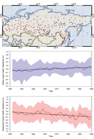
Figure 4.20. Variations in the thickness of the active layer over permafrost (middle) and maximum soil freeze depth in non-permafrost areas (bottom) in Russia from 1956 through 1990 . Active layer thickness has increased by about 20 cm while seasonal freeze depth has decreased by about 34 cm over the period of record (black lines in middle and lower panels). The anomaly in active layer thickness (blue line) is an average of anomalies from 31 stations (blue dots in the top panel) after removing the mean over the period of record for each station. The anomaly in maximum soil freeze depth (red line) is an average of anomalies from 211 stations (red dots in the top panel) after removing the mean over the period of record for each station. The shaded area represents the 5 to 95% confidence interval from the mean for each year, and the dashed line is the zero reference (from Frauenfeld et al., 2004 [JoC, SRC] ).
Long-term monitoring of the active layer has been conducted over the past several decades in Russia. By the early 1990 s, there were about 25 stations, each containing 8 to 10 plots and 20 to 30 boreholes to a depth of 10 to 15 m ( Pavlov, 1996 [MoS] ). Measurements of soil temperature in the active layer and permafrost at depths up to 3.20 m have been carried out in Russia from 31 hydrometeorological stations, most of them started in the 1950 s but a few as early as in the 1930 s( Figure 4.20 ). Active layer thickness can be estimated using these daily soil temperature measurements. Over the period 1956 to 1990, the active layer exhibited a statistically significant deepening of about 21 cm. Increases in summer air temperature and winter snow depth are responsible for the increase in active layer thickness.
Monitoring of the active layer was developed at a global scale in the 1990 s and currently incorporates more than 125 sites in the Arctic, the Antarctic and several mid-latitude mountain ranges ( Brown et al., 2000 [JoC, SRC] ;( Nelson, 2004a, ) b; Figure 4.21 ). These sites were designed to observe the response of the active layer and near-surface permafrost to climate change. The results from northern high-latitude sites demonstrate substantial interannual and inter-decadal fluctuations in active layer thickness in response to air temperature variations. During the mid- to late 1990 s in Alaska and north-western Canada, maximum and minimum thaw depths were observed in 1998 and in 2000, corresponding to the warmest and coolest summers, respectively. There is evidence of an increase in active layer thickness and thermokarst development, indicating degradation of warmer permafrost ( Brown et al., 2000 [JoC, SRC] ). Evidence from European monitoring sites indicates that active layer thickness has been the greatest in the summers of 2002 and 2003, approximately 20% greater than in previous years ( Harris et al., 2003 [JoC, SRC] ). Active layer thickness has increased by up to 1.0 m along the Qinghai-Xizang Highway over the Tibetan Plateau since the early 1980 s ( Zhao et al., 2004 [JoC, SRC] ).
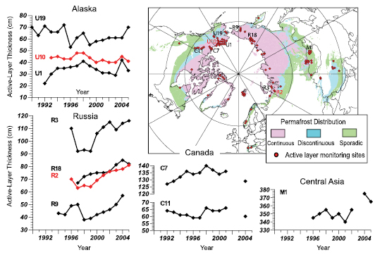
Figure 4.21. Locations of sites and changes in active layer thickness from selected sites (after ( Nelson, 2004a, ) b).
4.7.3.2 Seasonally Frozen Ground in Non-Permafrost Areas
The thickness of seasonally frozen ground has decreased by more than 0.34 m from 1956 through 1990 in Russia( Figure 4.20 ), primarily controlled by the increase in winter air temperature and snow depth ( Frauenfeld et al., 2004 [JoC, SRC] ). Over the Tibetan Plateau, the thickness of seasonally frozen ground has decreased by 0.05 to 0.22 m from 1967 through 1997 ( Zhao et al., 2004 [JoC, SRC] ). The driving force for the decrease in thickness of the seasonally frozen ground is the significant warming in cold seasons, while changes in snow depth play a minor role. The duration of seasonally frozen ground decreased by more than 20 days from 1967 through 1997 over the Tibetan Plateau, mainly due to the earlier onset of thaw in spring ( Zhao et al., 2004 [JoC, SRC] ).
The estimated maximum extent of seasonally frozen ground has decreased by about 7% in the NH from 1901 to 2002, with a decrease in spring of up to 15%( Figure 4.22 ;Zhang et al., 2003 [NPR, SRC] ). There was little change in the areal extent of seasonally frozen ground during the early and midwinters.
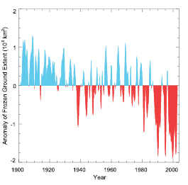
Figure 4.22. Historical variations in the monthly areal extent (106 km2)of seasonally frozen ground (including the active layer over permafrost) for the period from 1901 through 2002 in the NH. The positive anomaly (blue) represents above-average monthly extent, while the negative anomaly (red) represents below-average extent. The time series is smoothed with a low-pass filter (after Zhang et al., 2003 [NPR, SRC] ).
4.7.3.3 Near-Surface Soil Freeze-Thaw Cycle
Satellite remote sensing data have been used to detect the near-surface soil freeze-thaw cycle at regional and hemispheric scales. Evidence from the satellite record indicates that the onset dates of thaw in spring and freeze in autumn advanced five to seven days in Eurasia over the period 1988 to 2002, leading to an earlier start to the growing season but no change in its length ( Smith et al., 2004 [JoC] ). In North America, a trend towards later freeze dates in autumn by about five days led, in part, to a lengthening of the growing season by eight days. Overall, the timing of seasonal thawing and subsequent initiation of the growing season in early spring has advanced by approximately eight days from 1988 to 2001 for the pan-arctic basin and Alaska ( (McDonald et al., 2004 ) ).
Table 4.6. Estimates of cryospheric contributions to sea level change.
| Cryospheric component | Sea Level Equivalent (mm yr–1) | |
|---|---|---|
| 1961–2003 | 1993–2003 | |
| Glaciers and Ice Caps | +0.32 to +0.68 | +0.55 to +0.99 |
| Greenland | –0.07 to +0.17 | +0.14 to +0.28 |
| Antarctica | –0.28 to +0.55 | –0.14 to +0.55 |
| Total (adding ranges) | –0.03 to +1.40 | +0.55 to +1.82 |
| Total (Gaussian errorsummation) | +0.22 to +1.15 | +0.77 to +1.60 |
4.8 Synthesis
Observations show a consistent picture of surface warming and reduction in all components of the cryosphere( FAQ 4.1 ,Figure 1), [1] except antarctic sea ice, which exhibits a small positive but insignificant trend since 1978 ( Figure 4.23 ).
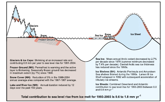
Since IPCC 2001 [NPR] ) the cryosphere has undergone significant changes, such as the substantial retreat of arctic sea ice, especially in summer; the continued shrinking of mountain glaciers; the decrease in the extent of snow cover and seasonally frozen ground, particularly in spring; the earlier breakup of river and lake ice; and widespread thinning of antarctic ice shelves along the Amundsen Sea coast, indicating increased basal melting due to increased ocean heat fluxes in the cavities below the ice shelves. An additional new feature is the increasingly visible fast dynamic response of ice shelves, for example, the dramatic breakup of the Larsen B Ice Shelf in 2002, and the acceleration of tributary glaciers and ice streams, with possible consequences for the adjacent part of the ice sheets.
One difficulty with using cryospheric quantities as indicators of climate change is the sparse historical database. Although ‘extent’ of ice (sea ice and glacier margins for example) has been observed for a long time at a few locations, the ‘amount’ of ice (thickness or depth) is difficult to measure. Therefore, reconstructions of past mass balance are often not possible.
The most important cryospheric contributions to sea level variations (see Chapter5 )arise from changes in the ice on land (e.g., glaciers, ice caps and ice sheets). In IPCC 2001 [NPR] ), the contribution of glaciers and ice caps to sea level rise during the 20th century was estimated as 0.2 to 0.4 mm yr–1 (of 1 to 2 mm yr–1 total sea level rise). New results presented here indicate that all glaciers contributed about 0.50 ± 0.18 mm yr–1 during 1961 to 2003, increasing to 0.77 ± 0.22 mm yr–1 from 1993 to 2003 (interpolation from five-year analyses in Table 4.4 ). Estimates for both ice sheets combined give a contribution ranging from –0.35 to +0.72 mm yr–1 for 1961 to 2003, increasing to 0 to 0.8 mm yr–1 for 1993 to 2003 . A conservative error estimate in terms of summing ranges is given in Table 4.6 .Assuming a midpoint mean, interpreting the range as uncertainty and using Gaussian error summation of estimates for glaciers and both ice sheets suggests that the total ice contribution to sea level rise was approximately 0.7 ± 0.5 mm yr–1 during 1961 to 2003 and 1.2 ± 0.4 mm yr–1 during 1993 to 2003 .
The large uncertainties reflect the difficulties in estimating the global ice mass and its variability, because global monitoring of ice thickness is impossible (even the total area of glaciers is not exactly known) and extrapolation from local measurements is therefore necessary. A regional extension of the monitored ice masses and an improvement of measurement and extrapolation techniques are urgently required.
In spite of the large uncertainties, the data that are available portray a rather consistent picture of a cryosphere in decline over the 20th century, increasingly so during 1993 to 2003 .
References
Abdalati, W., et al., 2001: Outlet glacier and margin elevation changes: Near-coastal thinning of the Greenland ice sheet. J. Geophys. Res., 106(D24), 33729–33741. [JoC]
Abdalati, W., et al., 2004: Elevation changes of ice caps in the Canadian Arctic Archipelago. J. Geophys. Res., 109,F04007, doi:10.1029/2003JF000045. [JoC]
Ackley, S., P. Wadhams, J.C. Comiso, and A.P. Worby, 2003: Decadal decrease of Antarctic sea ice extent inferred from whaling records revisited on the basis of historical and modern sea ice records. Polar Res., 22(1), 19–25. [SRC]
Agnew, T. and S. Howell, 2003: The use of operational ice charts for evaluating passive microwave ice concentration data. Atmos.-Ocean, 41(4), 317–331. Clean
Agnew, T., H. Le, and T. Hirose, 1997: Estimation of large-scale sea-ice motion from SSM/I 85.5 GHz imagery. Ann. Glaciol., 25,305–311. [MoS]
Allard, M., B. Wang, and J.A. Pilon, 1995: Recent cooling along the southern shore of Hudson Strait Quebec, Canada, documented from permafrost temperature measurements. Arctic and Alpine Res., 27,157–166. [ARC]
Alley, R.B., P.U. Clark, P. Huybrechts, and I. Joughin, 2005a: Ice-sheet and sea-level changes. Science, 310,456–460. [JoC, SRC]
Alley, R.B., T.K. Dupont, B.R. Parizek, and S. Anandakrishnan, 2005b: Access of surface meltwater to beds of sub-freezing glaciers: preliminary insights. Ann. Glaciol., 40,8–14. [SRC]
Arendt, A.A., et al., 2002: Rapid wastage of Alaska glaciers and their contribution to rising sea level. Science, 297,382–386. [JoC]
Armstrong, R.L. and M.J. Brodzik, 2001: Recent Northern Hemisphere snow extent: A comparison of data derived from visible and microwave satellite sensors. Geophys. Res. Lett., 28,3673–3676. [JoC]
Bamber, J.L., R.L. Layberry, and S.P. Gogineni, 2001: A new ice thickness and bed data set for the Greenland ice sheet, 1. Measurement, data reduction, and errors. J. Geophys. Res., 106,33733–33780. [JoC]
Bamber, J.L., W. Krabill, V. Raper, and J. Dowdeswell, 2004: Anomalous recent growth of part of a large Arctic ice cap: Austfonna, Svalbard. Geophys. Res. Lett., 31(12), L12402, doi: 10.1029/2004GL019667. [JoC]
Bamzai, A.S., 2003: Relationship between snow cover variability and Arctic Oscillation Index on a hierarchy of time scales. Int. J. Climatol., 23,131–142. [JoC]
Belchansky, G. I., D.C. Douglas, V.A. Eremeev, and N.G. Platonov, 2005: Variations in the Arctic’s multiyear sea ice cover: A neural network analysis of SMMR-SSM/I data, 1979-2004. Geophys. Res. Lett., 32,L09605, doi:10.1029/2005GL022395. [JoC]
Box, J.E., et al., 2006: Greenland ice-sheet surface mass balance variability (1988-2004) from calibrated Polar MM5 output. J. Clim., 19(12), 2783–2800. [JoC, SRC]
Broll, G., C. Tarnocai, and J. Gould, 2003: Long-term high Arctic ecosystem monitoring in Quttinirpaaq National Park, Ellesmere Island, Canada. In: Proceedings of the 8th International Conference on Permafrost, 21-25 July 2003, Zurich, Switzerland [Phillips, M., S.M. Springman, and L.U. Arenson (eds.)]. A.A. Balkema, Lisse, the Netherlands, pp. 89–94. [NPR]
Brown, J., K.M. Hinkel, and F.E. Nelson, 2000: The Circumpolar Active Layer Monitoring (CALM) program: research design and initial results. Polar Geogr., 24(3), 166–258. Clean
Brown, R.D., 2000: Northern hemisphere snow cover variability and change, 1915-97. J. Clim., 13,2339–2355. [JoC, SRC]
Brown, R.D., and P. Coté, 1992: Interannual variability of landfast ice thickness in the Canadian high Arctic, 1950-1989. Arctic, 45,273–284. [SRC]
Carrasco, J.F., G. Casassa, and J. Quintana, 2005: Changes of the 0°C isotherm and the equilibrium line altitude in central Chile during the last quarter of the XXth century. Hydrolog. Sci. J., 50,933–948. [SRC]
Cavalieri, D.J., 1992: The validation of geophysical products using multisensor data. In: Microwave Remote Sensing of Sea Ice [Carsey, F.D. (ed.)]. Geophysical Monograph 68, American Geophysical Union, Washington, DC, pp 233–242. [NPR]
Chinn, T.J.H., S. Winkler, M.J. Salinger, and N. Haakensen, 2005: Recent glacier advances in Norway and New Zealand: a comparison of their glaciological and meteorological causes. Geografiska Annaler, 87A(1), 141–157. Clean
Clare, G.R., B.B. Fizharris, T.J.H. Chinn, and M.J. Salinger, 2002: Interannual variation in end-of-summer snowlines of the Southern Alps of New Zealand, and relationships with Southern Hemisphere atmospheric circulation and sea surface temperature patterns. Int. J. Climatol., 22,107–120. [JoC]
Clark, M.P., M.C. Serreze, and D.A. Robinson, 1999: Atmospheric controls on Eurasian snow extent. Int. J. Climatol., 19,27–40. [JoC, SRC]
Clark, P.U., R.B. Alley, and D. Pollard, 1999: Northern hemisphere ice-sheet influences on global climate change. Science, 286,1103–1111. [JoC, SRC]
Cogley, J.G., 2005: Mass and energy balances of glaciers and ice sheets. In: Encyclopedia of Hydrological Sciences [Anderson, M. (ed.)]. John Wiley & Sons, Ltd, Chichester, pp 2555–2573. [NPR, SRC]
Comiso, J.C., 2002: A rapidly declining perennial sea ice cover in the Arctic. Geophys. Res. Lett., 29,1956–1959. [JoC, SRC]
Comiso, J.C., 2003: Large scale characteristics and variability of the global sea ice cover. In: Sea Ice - An Introduction to its Physics, Biology, Chemistry, and Geology [Thomas, D. and G.S. Dieckmann (eds.)]. Blackwell Science, Oxford, UK, pp. 112–142. [NPR, SRC]
Cook, A., A. Fox, D. Vaughan, and J. Ferigno, 2005: Retreating glacier fronts on the Antarctic Peninsula over the past half century. Science, 308,541–544. [JoC, SRC]
Couture, R., et al., 2003: On the hazards to infrastructure in the Canadian North associated with thawing of permafrost. In: Proceedings of Geohazards 2003, 3rd Canadian Conference on Geotechnique and Natural Hazards.Canadian Geotechnical Society, Alliston, Ontario, pp. 97–104. [NPR]
Cuffey, K.M., 2001: Interannual variability of elevation on the Greenland ice sheet: effects of firn densification, and establishment of a benchmark. Journal of Glaciol., 47(158), 369–377. Clean
Cullen, N.J., et al., 2006: Kilimanjaro glaciers: Recent areal extent from satellite data and new interpretation of observed 20th century retreat rates. Geophys. Res. Lett., 33,L16502, doi:10.1029/2006GL027084. [JoC]
Curran, M.A.J., et al., 2003: Ice core evidence for Antarctic sea ice decline since the 1950s. Science, 302(14), 1203–1206. [JoC]
Davis, C.H., et al., 2005: Snowfall-driven growth in East Antarctic ice sheet mitigates recent sea-level rise. Science, 308,1898–1901, doi:10.1126/science.1110662. [JoC]
de la Mare, W.K., 1997: Abrupt mid-20th century decline in Antarctic sea ice extent from whaling records. Nature, 389,57–61. [JoC]
Derksen, C., A. Walker, E. LeDrew, and B. Goodison, 2003: Combining SMMR and SSM/I data for time series analysis of central North American snow water equivalent. J. Hydrometeorol., 4(2), 304–316. [JoC]
DesJarlais, C., 2004: S’adapter aux Changements Climatiques.Ouranos, Montreal, 91pp. [NPR]
Doran, P.T., et al., 2002: Antarctic climate cooling and terrestrial ecosystem response. Nature, 415,517–520. [JoC]
Duguay, C.R., et al., 2003: Ice-cover variability on shallow lakes at high latitudes: model simulations and observations. Hydrolog. Process., 17,3465–3483. [MoS]
Duguay, C.R., et al., 2006: Recent trends in Canadian lake ice cover. Hydrological Processes, 20,781–801. Clean
Dumas, J.A., G.M. Flato, and A.J. Weaver, 2003: The impact of varying atmospheric forcing on the thickness of arctic multi-year sea ice. Geophys. Res. Lett., 30(18), 1918–1921. [JoC, MoS, SRC]
Dupont, T.K., and R.B. Alley, 2005: Assessment of the importance of ice-shelf buttressing to ice-sheet flow. Geophys. Res. Lett., 32,L04503, doi:10.1029/2004GL022024. [JoC, SRC]
Dupont, T.K., and R.B. Alley, 2006: The importance of small ice shelves in sea-level rise. Geophys. Res. Lett., 33,L09503, doi:10.1029/2005GL025665. [JoC, SRC]
Dye, D.G., 2002: Variability and trends in the annual snow-cover cycle in Northern Hemisphere land areas, 1972–2000. Hydrolog. Process., 16,3065–3077. Clean
Dyurgerov, M., and J. Dwyer, 2000. The steepening of glacier mass balance gradients with Northern Hemisphere warming. Zeitschrift für Gletscherkunde und Glazialgeologie, 36,107–118. [SRC]
Dyurgerov, M., and M.F. Meier, 2005: Glaciers and the Changing Earth System: A 2004 Snapshot.Occasional Paper 58, Institute of Arctic and Alpine Research, University of Colorado, Boulder, CO, 118 pp. [NPR, SRC]
Falarz, M., 2002: Long-term variability in reconstructed and observed snow cover over the last 100 winter seasons in Cracow and Zakopane (southern Poland). Clim. Res., 19(3), 247–256. Clean
Favier, V., P. Wagnon, and P. Ribstein, 2004: Glaciers of the outer and inner tropics: A different behaviour but a common response to climatic forcing. Geophys. Res. Lett., 31,L16403, doi:10.1029/2004GL020654. [JoC, MoS]
Fedorov, A., and P. Konstantinov, 2003: Observations of surface dynamics with thermokarst initiation, Yukechi site, central Yakutia. In: Proceedings of the 8th International Conference on Permafrost, 21-25 July 2003, Zurich, Switzerland [Phillips, M., S.M. Springman, and L.U. Arenson (eds.)]. A.A. Balkema, Lisse, the Netherlands, pp. 239–243. [NPR]
Fichefet, T., B. Tartinville, and H. Goosse, 2003: Antarctic sea ice variability during 1958-1999: A simulation with a global ice-ocean model. J. Geophys. Res., 108(C3), 3102–3113. [JoC, MoS, ARC]
Fitzharris, B.B., and C.E. Garr, 1995: Simulation of past variability in seasonal snow in the Southern Alps, New Zealand. Ann. Glaciol., 21,377–382. [MoS, SRC]
Fountain, A.G., T.A. Neumann, P.L. Glenn, and T. Chinn, 2004: Can warming induce advances of polar glaciers, Taylor Valley, Antarctica. J. Glaciol., 50(171), 556–564. Clean
Francou, B., et al., 2003: Tropical climate change recorded by a glacier in the central Andes during the last decades of the twentieth century: Chacaltaya, Bolivia, 16°S. J. Geophys. Res., 108(D5), 4154, doi:10.1029/2002JD002959. [JoC]
Francou, B., M. Vuille, V. Favier, and B. Cáceres, 2004: New evidence for an ENSO impact on low-latitude glaciers: Antizana 15, Andes of Ecuador, 0°28’S. J. Geophys. Res., 109,D18106, doi:10.1029/2003JD004484. [JoC]
Frauenfeld, O.W., T. Zhang, R.G. Barry, and D. Gilichinsky, 2004: Interdecadal changes in seasonal freeze and thaw depths in Russia. J. Geophys. Res., 109,D5101, doi:10.1029/2003JD004245. [JoC, SRC]
Fujita, K., and Y. Ageta, 2000: Effect of summer accumulation on glacier mass balance on the Tibetan Plateau revealed by mass-balance model. J. Glaciol., 46(153), 244–252. [MoS]
Gavrilov, P.P. and P.V. Efremov, 2003: Effects of cryogenic processes on Yakutia landscapes under climate warming. In: Proceedings of the 8th International Conference on Permafrost, 21-25 July 2003, Zurich, Switzerland [Phillips, M., S.M. Springman, and L.U. Arenson (eds.)]. A.A. Balkema, Lisse, the Netherlands, pp. 277–282. [NPR]
Georges, C., 2004: The 20th century glacier fluctuations in the Cordillera Blanca (Perú). Arctic, Antarctic, and Alpine Res., 36(1), 100–107. Clean
Greene, A.M., 2005: A time constant for hemispheric glacier mass balance. J. Glaciol., 51(174), 353–362. Clean
Groisman, P.Ya, T.R. Karl, and R.W. Knight, 1994: Observed impact of snow cover on the heat balance and the rise of continental spring temperatures. Science, 263,198–200. [PoC, JoC, ARC]
Groisman, P.Ya., et al., 2004: Contemporary changes of the hydrological cycle over the contiguous United States: Trends derived from in situ observations. J. Hydrometeorol., 5,64–85. [JoC, ARC]
Gudkovich, Z.M., 1961: Relation of the ice drift in the Arctic Basin to ice conditions in the Soviet Arctic seas. Tr. Okeanogr. Kom. Akad. Nauk SSSR, 11,14–21 (in Russian). Clean
Haas, C., 2004: Late-summer sea ice thickness variability in the Arctic Transpolar Drift 1991–2001 derived from ground-based electromagnetic sounding. Geophys. Res. Lett., 31,L09402, doi:10.1029/2003GL019394. [JoC, SRC]
Haeberli, W., and C.R. Burn, 2002: Natural hazards in forests: glacier and permafrost effects as related to climate change. In: Environmental Change and Geomorphic Hazards in Forests [Sidle, R.C. (ed.)]. IUFRO Research Series 9, CABI Publishing, Wallingford and New York, pp. 167–202. [NPR]
Hagen, J.O., K. Melvold, F. Pinglot, and J.A. Dowdeswell, 2003: On the net mass balance of the glaciers and ice caps in Svalbard, Norwegian Arctic. Arctic, Antarctic, and Alpine Res., 35(2), 264–270. [SRC]
Halsey, L.A., D.H. Vitt, and S.C. Zoltai, 1995: Disequilibrium response of permafrost in boreal continental western Canada to climate change. Clim. Change, 30,57–73. [JoC]
Hanna, E., et al., 2005: Runoff and mass balance of the Greenland ice sheet: 1958-2003. J. Geophys. Res., 110,D13108, doi:10.1029/2004JD005641. [JoC]
Hanna, E., et al., 2006: Observed and modeled Greenland Ice Sheet snow accumulation, 1958–2003, and links with regional climate forcing. J. Clim., 19(3), 344–358. [JoC, MoS]
Hansen, J., and L. Nazarenko, 2004: Soot climate forcing via snow and ice albedos. Proc. Natl. Acad. Sci. U.S.A., 101(2), 423–428. [JoC, MoS, ARC]
Harris, C., et al., 2003: Warming permafrost in European mountains. Global Planet. Change, 39,215–225. [JoC, SRC]
Hastenrath, S., 2005: The glaciers of Mount Kenya 1899-2004. Erdkunde, 59,120–125. Clean
Heil, P., and I. Allison, 2002: Long-term fast-ice variability off Davis and Mawson stations, Antarctica. In: Ice in the Environment: Proceedings of the 16th IAHR International Symposium on Ice (Volume 1), Dunedin, New Zealand, 2-6 December 2002 [Squire, V., and P. Langhorne (eds)]. University of Otago, Dunedin, NZ, pp. 360–367. [NPR, SRC]
Hellmer, H., S. Jacobs, and A. Jenkins, 1998: Oceanic erosion of a floating Antarctic glacier in the Amundsen Sea. In: Ocean, Ice, and Atmosphere: Interactions at the Antarctic Continental Margin [Jacobs, S. and R. Weiss (eds.)]. Antarctic Research Series 75, American Geophysical Union, Washington, DC, pp. 83–99. [NPR, SRC]
Hennessy, K.J., et al., 2003: The Impact of Climate Change on Snow Conditions in Mainland Australia.CSIRO Atmospheric Research, Aspendale, Australia, 47 pp, http://www.cmar.csiro.au/e-print/open/hennessy_2003a.pdf. [NPR]
Hewitt, K., 2005: The Karakoram anomaly? Glacier expansion and the “elevation effect”, Karakoram Himalaya. Mountain Research and Development, 25(4), 332–340. Clean
Hill, B.T., A. Ruffman, and K. Drinkwater. 2002: Historical record of the incidence of sea ice on the Scotian Shelf and the Gulf of St. Lawrence. In: Ice in the Environment: Proceedings of the 16th IAHR International Symposium on Ice (Volume 1). Dunedin, New Zealand, 2-6 December 2002 [Squire, V., and P. Langhorne (eds)]. University of Otago, Dunedin, NZ. [NPR]
Hilmer, M., and T. Jung, 2000: Evidence for a recent change in the link between the North Atlantic Oscillation and Arctic sea ice export. Geophys. Res. Lett., 27,989–992. [JoC]
Hinzman, L.D., et al., 2003: Hydrological variations among watersheds with varying degrees of permafrost. Proceedings of the 8th International Conference on Permafrost, 21-25 July 2003, Zurich, Switzerland [Phillips, M., S.M. Springman, and L.U. Arenson (eds.)]. A.A. Balkema, Lisse, the Netherlands, pp. 407–411. [NPR, SRC]
Hinzman, L.D., et al., 2005: Evidence and implications of recent climate change in northern Alaska and other arctic regions. Clim. Change, 72(3), 251–298. [JoC, SRC]
Holloway, G., and T. Sou, 2002: Has Arctic sea ice rapidly thinned? J. Clim., 15,1691–1701. [JoC]
Howat, I.M., I. Joughin, S. Tulaczyk, and S. Gogineni, 2005: Rapid retreat and acceleration of Helheim Glacier, east Greenland. Geophys. Res. Lett., 32,L22502, doi: 10.1029/2005GL024737. [JoC, SRC]
Huybrechts, P., 2002: Sea-level changes at the LGM from ice-dynamic reconstructions of the Greenland and Antarctic ice sheets during the glacial cycles. Quat. Sci. Rev., 21(1–3), 203–231. [JoC, SRC]
Huybrechts, P., J. Gregory, I. Janssens, and M. Wild, 2004: Modelling Antarctic and Greenland volume changes during the 20th and 21st centuries forced by GCM time slice integrations. Global Planet. Change, 42(1–4), 83–105. [JoC, MoS, SRC]
Hyvärinen, V., 2003: Trends and characteristics of hydrological time series in Finland. Nord. Hydrol., 34(1–2), 71–90. Clean
IPCC, 2001: Climate Change 2001: The Scientific Basis. Contribution of Working Group I to the Third Assessment Report of the Intergovernmental Panel on Climate Change [Houghton, J.T., et al. (eds)]. Cambridge University Press, Cambridge, United Kingdom and New York, NY, USA, 881 pp. [NPR]
Isaksen, K., P. Holmlund, J.L. Sollid, and C. Harris, 2001: Three deep alpine-permafrost boreholes in Svalbard and Scandinavia. Permafrost and Periglacial Processes, 12,13–25. [SRC]
Jacka, T.H., et al., 2004: Recommendations for the collection and synthesis of Antarctic Ice Sheet mass balance data. Global Planet. Change, 42(1–4), 1–15. [JoC]
Jacobs, S.S., C.F. Giulivi, and P.A. Mele, 2002: Freshening of the Ross Sea during the late 20th century. Science, 297(5580), 386–389. [JoC]
Johannessen, O.M, E.V. Shalina, and M.W. Miles, 1999: Satellite evidence for an Arctic sea ice cover in transformation. Science,286, 1937–1939. [JoC]
Johannessen, O.M., K. Khvorostovsky, M.W. Miles, and L.P. Bobylev, 2005: Recent ice-sheet growth in the interior of Greenland. Science, 310,1013–1016. [JoC]
Johannessen, O.M., et al., 2004: Arctic climate change – observed and modelled temperature and sea ice. Tellus, 56A,328–341. [JoC, MoS]
Jones, P.D., and A. Moberg, 2003: Hemispheric and large-scale surface air temperature variations: an extensive revision and an update to 2001. JClimate, 16,206–223. [ARC]
Jorgenson, M.T., and J. Brown, 2005: Classification of the Alaskan Beaufort Sea Coast and estimation of carbon and sediment inputs from coastal erosion. Geo-Marine Lett., 25,69–80. [MoS]
Joughin, I., and S. Tulaczyk, 2002: Positive mass balance of the Ross Ice Streams, West Antarctica. Science, 295(5554), 476–480. [JoC, SRC]
Joughin, I., and L. Padman, 2003: Melting and freezing beneath Filchner-Ronne Ice Shelf, Antarctica. Geophys. Res. Lett., 30(9), 1477, doi:10.1029/2003GL016941. [JoC, SRC]
Joughin, I., W. Abdalati, and M. Fahnestock, 2004: Large fluctuations in speed on Greenland’s Jakobshavn Isbræ glacier. Nature, 432,608–610. [JoC, SRC]
Joughin, I., et al., 2003: Timing of recent accelerations of Pine Island Glacier, Antarctica. Geophys. Res. Lett., 30(13), 1706, doi:10.1029/2003GL017609. [JoC, SRC]
Kane, D.L., L.D. Hinzman, and J.P. Zarling, 1991: Thermal response of the active layer to climate warming in a permafrost environment. Cold Regions Sci. Technol., 19,111–122. [SRC]
Kaser, G., and H. Osmaston, 2002: Tropical Glaciers.UNESCO International Hydrological Series. Cambridge University Press, Cambridge, UK, 207pp. [NPR, SRC]
Kaser, G., et al., 2003: The impact of glaciers on the runoff and the reconstruction of mass balance history from hydrological data in the tropical Cordillera Blanca, Peru. J. Hydrol., 282,130–144. [SRC]
Kjøllmoen, B.E., 2005: Glaciological Investigations in Norway in 2004.Norwegian Water Resources and Energy Directorate, Oslo, http://www.nve.no/FileArchive/176/Glac_invest2004.pdf. [NPR]
Klein, A.G., and J.L. Kincaid, 2006: Retreat of glaciers on Puncak Jaya, Irian Jaya, determined from 2000 and 2002 IKONOS satellite images. J. Glaciol., 52(176), 65–79. Clean
Koeberle, C., and R. Gerdes, 2003: Mechanisms determining the variability of Arctic sea ice conditions and export. J. Clim., 16,2843–2858. [JoC, ARC]
Krabill, W.B., et al., 2000: Greenland Ice Sheet: High elevation balance and peripheral thinning. Science, 289,428–430. [JoC]
Krabill, W.B., et al., 2002: Aircraft laser altimetry measurement of elevation changes of the Greenland ice sheet: Technique and accuracy assessment. J. Geodyn., 34,357–376. Clean
Krabill, W.B., et al., 2004: Greenland Ice Sheet: Increased coastal thinning. Geophys. Res. Lett., 31,L24402, doi:10.1029/2004GL021533. [JoC]
Kwok, R., 2000: Recent changes of the Arctic Ocean sea ice motion associated with the North Atlantic Oscillation. Geophys. Res. Lett, 27(6), 775–778. [JoC, SRC]
Kwok, R., 2002: Sea ice concentration from passive microwave radiometry and openings from SAR ice motion. Geophys. Res. Lett, 29(10), doi:10.1029/2002GL014787. [JoC, SRC]
Kwok, R., and D.A. Rothrock, 1999: Variability of Fram Strait ice flux and North Atlantic Oscillation. J. Geophys. Res., 104,5177–5189. [JoC, SRC]
Kwok, R., G.F. Cunningham, and S.S. Pang, 2004: Fram Strait sea ice outflow. J. Geophys. Res., 109,C01009, doi:10.1029/2003JC001785. [JoC, SRC]
Kwok, R., et al., 1998: Assessment of sea ice motion from sequential passive microwave observations with ERS and buoy ice motions. J. Geophys. Res., 103(C4), 8191–8213. [JoC, SRC]
Lachenbruch, A.H., and B.V. Marshall, 1986: Changing climate: geothermal evidence from permafrost in the Alaskan Arctic. Science, 234,689–696. [JoC]
Laxon, S., N. Peacock, and D. Smith, 2003: High interannual variability of sea ice thickness in the Arctic region. Nature, 425,947–950. [JoC, SRC]
Legresy, B., F. Remy, and F. Blarel, 2006: Along track repeat altimetry for ice sheets and continental surface studies. In: Proceedings of the Symposium on 15 years of Progress in Radar Altimetry, Venice, Italy, 13-18 March 2006 [Danesy, D. (ed.)]. ESA-SP614, Paper 181, European Space Agency Publications Division, Noordwijk, The Netherlands, 4 pp., http://earth.esa.int/workshops/venice06/participants/181/paper_181_legrsy.pdf. [NPR]
Lewkowicz, A.G., 1992: Factors influencing the distribution and initiation of active-layer detachment slides on Ellesmere Island, arctic Canada. In: Periglacial Geomorphology [Dixon, J.C. and A.D. Abrahams (eds.)]. Wiley, New York, pp. 223–250. [NPR]
Liu, S., et al., 2004: Recent progress in glaciological studies in China. J. Geogr. Sci., 14(4), 401–410. [SRC]
Lo, F., and M.P. Clark, 2001: Relationships between spring snow mass and summer precipitation in the southwestern US associated with the North American monsoon system. J. Clim., 15,1378–1385. [JoC]
Lythe, M.B., D.G. Vaughan, and the BEDMAP Group, 2001: BEDMAP: A new ice thickness and subglacial topographic model of Antarctica. J. Geophys. Res., 106(B6), 11335–11351. [JoC, MoS, SRC]
Magnuson, J.J., et al., 2000: Historical trends in lake and river ice cover in the Northern Hemisphere. Science, 289,1743–1746. [JoC]
Massom, R.A., et al., 2001: Snow on Antarctic sea ice: a review of physical characteristics.Rev. Geophys., 39(3), 413–445 Clean
McDonald, K.C., et al., 2004: Variability in springtime thaw in the terrestrial high latitudes: monitoring a major control on the biospheric assimilation of atmospheric CO2 with spaceborne microwave remote sensing. Earth Interactions, 8,Paper No. 20. Clean
McLaren, A.S., R.H. Bourke, J.E. Walsh, and R.L. Weaver, 1994: Variability in sea-ice thickness over the North Pole from 1958 to 1992. In: The Polar Oceans and Their Role in Shaping the Global Environment [Johannessen, O.M., R.D. Muench, and J.E. Overland (eds.)]. American Geophysical Union, Washington, DC, pp. 363–371. [NPR, SRC]
Mitrovica, J.X., et al., 2006: Reanalysis of ancient eclipse, astronomic and geodetic data: A possible route to resolving the enigma of global sea level rise. Earth Planet. Sci. Lett., 243,390–399. Clean
Mölg, T., and D.R. Hardy, 2004: Ablation and associated energy balance of a horizontal glacier surface on Kilimanjaro. J. Geophys. Res., 109,1–13, D16104, doi:10.1029/2003JD004338. [JoC]
Mölg, T., C. Georges, and G. Kaser, 2003a: The contribution of increased incoming shortwave radiation to the retreat of the Rwenzori Glaciers, East Africa, during the 20th century. Int. J. Climatol., 23,291–303, doi:10.1002/joc.877. [JoC, SRC]
Mölg, T., D.R. Hardy, and G. Kaser, 2003b: Solar-radiation-maintained glacier recession on Kilimanjaro drawn from combined ice-radiation geometry modeling. J. Geophys. Res., 108(D23), 4731, doi:10.1029/2003JD003546. [JoC, MoS, SRC]
Monaghan, A.J., et al., 2006: Insignificant change in Antarctic snowfall since the International Geophysical Year. Science, 313(5788), 827–831. [JoC]
Morris, E.M., and D. G. Vaughan, 2003: Glaciological climate relationships spatial and temporal variation of surface temperature on the Antarctic Peninsula and the limit of viability of ice shelves. In: Antarctic Peninsula Climate Variability: Historical and Paleoenvironmental Perspectives [Domack, E., et al. (eds.)]. Antarctic Research Series 79, American Geophysical Union, Washington, DC, pp. 61–68. [NPR, SRC]
Mote, P.W., 2006: Climate-driven variability and trends in mountain snowpack in western North America. J. Clim., 19(23), 6209–6220. [JoC, SRC]
Mote, P.W., A.F. Hamlet, M.P. Clark, and D.P. Lettenmaier, 2005: Declining mountain snowpack in western North America. Bull. Am. Meteorol. Soc., 86,39–49, doi:10.1175/BAMS-86-1-39. [JoC, SRC]
Munk, W., 2002: Twentieth century sea level: An enigma. Proc. Natl. Acad. Sci. U.S.A., 99,6550–6555. [JoC]
Murphy, E.J., A. Clarke, C. Symon, and J. Priddle, 1995: Temporal variation in Antarctic sea-ice: analysis of a long term fast-ice record from the South Orkney Islands. Deep-Sea. Res., 42,l045–1062. Clean
Nagurnyi, A.P., V.G. Korostolev, and V.V. Ivanov, 1999: Multiyear variability of sea ice thickness in the Arctic basin measured by elastic-gravity waves on the ice surface. Meteorol. Hydrol., 3,72–78 (in Russian). Clean
Nan, Z., Z. Gao, S. Li, and T. Wu, 2003: Permafrost changes in the northern limit of permafrost on the Qinghai-Tibet Plateau in the last 30 years. Acta Geogr. Sin., 58(6), 817–823 (in Chinese). Clean
Nelson, F.E., O.A. Anisimov, and N.I. Shiklomanov, 2001: Subsidence risk from thawing permafrost. Nature, 410,889–890. [JoC]
Nelson, F.E. (ed.), 2004a: Circumpolar Active Layer Monitoring (CALM) Workshop. Permafrost and Periglacial Processes, 15(2), 99–188. Clean
Nelson, F.E. (ed.), 2004b: Eurasian contributions to the Circumpolar Active Layer Monitoring (CALM) Workshop. Polar Geogr., 28(4), 253–340. Clean
Nesje, A., and S.O. Dahl, 2003: The ‘Little Ice Age’ - only temperature? The Holocene, 13(1), 139–145. [JoC]
Nesje, A., Ø. Lie, and S.O. Dahl, 2000: Is the North Atlantic Oscillation reflected in Scandinavian glacier mass balance records? J. Quat. Sci., 15(6), 587–601. Clean
Nicholls, N., 2005: Climate variability, climate change and the Australian snow season. Aust. Meteorol. Mag., 54,177–185. [ARC]
Oberman, N.G., and G.G. Mazhitova, 2001: Permafrost dynamics in the northeast of European Russia at the end of the 20th century. Norwegian J. Geogr., 55,241–244. Clean
Oerlemans, J., 2005: Extracting a climate signal from 169 glacier records. Science, 308,675-677. [JoC, ARC]
Ohmura, A., 2001: Physical basis for the temperature/melt-index method. J. Appl. Meteorol., 40,753–761. [JoC, SRC]
Ohmura, A., 2004: Cryosphere during the twentieth century. In: The State of the Planet: Frontiers and Challenges in Geophysics [Sparks, R.S.J. and C.J. Hawkesworth (eds.)]. Geophysical Monograph 150, International Union of Geodesy and Geophysics, Boulder, CO and American Geophysical Union, Washington, DC, pp. 239–257. [NPR, SRC]
Omstedt, A., and D. Chen, 2001: Influence of atmospheric circulation on the maximum ice extent in the Baltic Sea. J. Geophys. Res., 106,4493–4500. [JoC]
Osterkamp, T.E., 2003: A thermal history of permafrost in Alaska. In: Proceedings of the 8th International Conference on Permafrost, 21-25 July 2003, Zurich, Switzerland [Phillips, M., S.M. Springman, and L.U. Arenson (eds.)]. A.A. Balkema, Lisse, the Netherlands, pp. 863–867. [NPR]
Osterkamp, T.E., 2005: The recent warming of permafrost in Alaska. Global Planet. Change, 49,187–202, doi: 10.1016/j.gloplacha.2005.09.001. [JoC]
Parizek, B.R., and R.B. Alley, 2004: Implications of increased Greenland surface melt under global-warming scenarios: ice-sheet simulations. Quat. Sci. Rev., 23(9–10), 1013–1027. [JoC, MoS, SRC]
Parizek, B.R., R.B. Alley, and C.L. Hulbe, 2003: Subglacial thermal balance permits ongoing grounding-line retreat along the Siple Coast of West Antarctica. Ann. Glaciol., 36,251–256. [SRC]
Parkinson, C.L., 1990: Search for the Little Ice Age in Southern Ocean sea-ice records. Ann. Glaciol., 14,221–225. Clean
Paterson, W.S.B., 2004: The Physics of Glaciers,Ed. 3.A, Elsevier, Oxford, UK, 496pp. [NPR]
Pavlov, A.V., 1996: Permafrost-climate monitoring of Russia: analysis of field data and forecast. Polar Geogr., 20(1), 44–64. [MoS]
Payne, A.J., et al., 2004: Recent dramatic thinning of largest West Antarctic ice stream triggered by oceans. Geophys. Res. Lett., 31,L23401, doi:10.1029/2004GL021284. [JoC, SRC]
Peltier, W.R., 1998: Postglacial variations in the level of the sea: implications for climate dynamics and solid-earth geophysics. Rev. Geophys., 36,603–689. [JoC]
Petkova, N., E. Koleva, and V. Alexandrov, 2004: Snow cover variability and change in mountainous regions of Bulgaria, 1931-2000. Meteorol. Z., 13(1), 19–23. Clean
Pettersson, R., P. Jansson, and P. Holmlund, 2003: Cold surface layer thinning on Storglaciären, Sweden, observed by repeated ground penetrating radar surveys. J. Geophys. Res., 108(F1), 6004, doi:10.1029/2003JF000024. [JoC, SRC]
Polyakov, I.V., et al., 2003: Long-term ice variability in Arctic marginal seas. J. Clim., 16,2078–2085. [JoC]
Prieto, R, et al., 2001: Interannual oscillations and trend of snow occurrence in the Andes region since 1885. Aust. Meteorol. Mag., 50(2), 164. Clean
Proshutinsky, A.Y., and M.A. Johnson, 1997: Two circulation regimes of the wind-driven Arctic Ocean. J. Geophys. Res., 102(C6), 12493–12514. [JoC, ARC]
Qin, D., S. Liu, and P. Li, 2006: Snow cover distribution, variability, and response to climate change in Western China. J. Clim., 19,1820–1833. [JoC, SRC]
Qiu, G., Y. Zhou, D. Guo, and Y. Wang, 2000: The map of geocryological regionalization and classification in China. In: Geocryology in China [Zhou, Y., D. Guo, G. Qiu, G. Cheng, and S. Li (eds.)]. Science Press, Beijing (in Chinese). The digital version of the map is available at the National Snow and Ice Data Center, University of Colorado at Boulder, Boulder, CO, http://nsidc.org/data/ggd603.html. [NPR]
Rachold, V., et al., 2003: Modern terrigenous organic carbon input to the Arctic Ocean. In: Organic Carbon Cycle in the Arctic Ocean: Present and Past [Stein, R., and R.W. Macdonald (eds.)]. Springer Verlag, Berlin, pp. 33–55. [NPR]
Ramillien, G., et al., 2006: Interannual variations of the mass balance of the Antarctica and Greenland ice sheets from GRACE. Global Planet. Change, 53,198–208. [JoC]
Randerson, J.T., C.B. Field, I.Y. Fung, and C.B. Tans, 1999: Increases in early season ecosystem uptake explain recent changes in the seasonal cycle of the atmospheric CO2 at high northern latitudes. Geophys. Res. Lett., 26,2765–2768. [JoC, ARC]
Raper, S.C.B., and R.J. Braithwaite, 2005: The potential for sea level rise: New estimates from glacier and ice cap area and volume distribution. Geophys. Res. Lett., 32,L05502, doi:10.1029/2004GL021981. [JoC, MoS, ARC]
Rayner, N.A., et al., 2003: Global analyses of sea surface temperature, sea ice and night marine air temperature since the late nineteenth century. J. Geophys. Res., 108(D14), 4407, doi: 10.1029/2002JD002670. [JoC]
Ren, J., et al., 2004: Glacier variations and climate warming and drying in the central Himalayas. Chin. Sci. Bull., 49(1), 65–69. [SRC]
Rignot, E., and S. Jacobs, 2002: Rapid bottom melting widespread near Antarctic Ice Sheet grounding lines. Science, 296,2020–2023. [JoC, SRC]
Rignot, E., and R.H. Thomas, 2002: Mass balance of polar ice sheets. Science, 297(5586), 1502–1506. [JoC, SRC]
Rignot, E., and P. Kanagaratnam, 2006: Changes in the velocity structure of the Greenland Ice Sheet. Science, 311,986–990. [JoC, SRC]
Rignot, E., A. Rivera, and G. Casassa, 2003: Contribution of the Patagonia Icefields of South America to sea level rise. Science, 302,434–437. [JoC, SRC]
Rignot, E., et al., 2004: Accelerated ice discharge from the Antarctic Peninsula following the collapse of Larsen B ice shelf. Geophys. Res. Lett., 31(18), L18401, doi:10.1029/2004GL020697. [JoC, SRC]
Rignot, E., et al., 2005: Recent ice loss from the Fleming and other glaciers, Wordie Bay, West Antarctic Peninsula. Geophys. Res. Lett., 32(7), 1–4. [JoC, SRC]
Rigor, I.G., J.M. Wallace, and R.L. Colony, 2002: Response of sea ice to the arctic oscillation. J. Clim., 15,2648– 2663. [JoC, SRC]
Robertson, R., M. Visbek, A. Gordon, and E. Fahrbach, 2002: Long term temperature trends in the deep waters of the Weddell. Deep-Sea Res., 49,4791–4802. Clean
Robinson, D.A., and A. Frei, 2000: Seasonal variability of northern hemisphere snow extent using visible satellite data. Professional Geogr., 51,307–314. [SRC]
Robinson, D.A., K.F. Dewey, and R.R. Heim Jr., 1993: Global snow cover monitoring: an update. Bull. Am. Meteorol. Soc., 74,1689–1696. [JoC, SRC]
Robock, A., M. Mu, K. Vinnikov, and D. Robinson, 2003: Land surface conditions over Eurasia and Indian summer monsoon rainfall. J. Geophys. Res., 108(D4), 4131, doi: 10.1029/2002JD002286. [JoC, SRC]
Romanovsky, V.E., et al., 2002: Permafrost temperature records: Indicator of climate change. Eos, 83(50), 589, 593–594. [JoC]
Rothrock, D.A., Y. Yu, and G.A. Maykut, 1999: Thinning of the Arctic sea-ice cover. Geophys. Res. Lett., 26(23), 3469. [JoC, SRC]
Rothrock, D.A., J. Zhang, and Y. Yu., 2003: The arctic ice thickness anomaly of the 1990s: A consistent view from observations and models. J. Geophys. Res., 108(C3), 3083, doi:10.1029/2001JC001208. [JoC, MoS, SRC]
Saito, K., and J. Cohen, 2003: The potential role of snow cover in forcing interannual variability of the major Northern Hemisphere mode. Geophys. Res. Lett., 30,1302, doi:10.1029/2002GL016341. [JoC, MoS]
Scambos, T., C. Hulbe, and M. Fahnestock, 2003: Climate-induced ice shelf disintegration in the Antarctic Peninsula. In: Antarctic Peninsula Climate Variability: Historical and Paleoenvironmental Perspectives [Domack, E., et al. (eds.)]. Antarctic Research Series 79, American Geophysical Union, Washington, DC, pp. 79–92. [NPR]
Scambos, T., C. Hulbe, M. Fahnestock, and J. Bohlander, 2000: The link between climate warming and break-up of ice shelves in the Antarctic Peninsula. J. Glaciol., 46,516–530. Clean
Scambos, T., J. Bohlander, C. Shuman, and P. Skvarca, 2004: Glacier acceleration and thinning after ice shelf collapse in the Larsen B embayment, Antarctica. Geophys. Res. Lett., 31,L18401, doi:10.1029/2004GL020670. [JoC]
Scherrer, S.C., C. Appenzeller, and M. Laternser, 2004: Trends in Swiss alpine snow days – the role of local and large scale climate variability. Geophys. Res. Lett., 31,L13215, doi:10.1029/2004GL020255. [JoC, SRC]
Schmitt, C., Ch. Kottmeier, S. Wassermann, and M. Drinkwater, 2004: Atlas of Antarctic Sea Ice Drift.University of Karlsruhe, Karlsruhe, http://imkhp7.physik.uni-karlsruhe.de/~eisatlas/eisatlas_start.html. [NPR, SRC]
Schneider, D.P., E.J. Steig, and J.C. Comiso, 2004: Recent climate variability in Antarctica from satellite-derived temperature data. J. Clim., 17,1569–1583. [JoC, SRC]
Sharkhuu, N., 2003: Recent changes in the permafrost of Mongolia. In: Proceedings of the 8th International Conference on Permafrost, 21-25 July 2003, Zurich, Switzerland [Phillips, M., S.M. Springman, and L.U. Arenson (eds.)]. A.A. Balkema, Lisse, the Netherlands, pp. 1029–1034. [NPR]
Shepherd, A., D.J. Wingham, and J.A.D. Mansley, 2002: Inland thinning of the Amundsen Sea sector, West Antarctica. Geophys. Res. Lett., 29(10), 1364. [JoC, ARC]
Shepherd, A., D. Wingham, and E. Rignot, 2004: Warm ocean is eroding West Antarctic Ice Sheet. Geophys. Res. Lett., 31(23), 1–4. [JoC, SRC]
Shepherd, A., D. Wingham, T. Payne, and P. Skvarca, 2003: Larsen Ice Shelf has progressively thinned. Science, 302,856–859. [JoC, ARC]
Shy, T.L., and J.E. Walsh, 1996: North Pole ice thickness and association with ice motion history. Geophys. Res. Lett., 23(21), 2975–2978. [JoC, SRC]
Sicart, J.E., P. Wagnon, and P. Ribstein, 2005: Atmospheric controls of the heat balance of Zongo Glacier (16°S, Bolivia). J. Geophys. Res., 110,D12106, doi:10.1029/2004JD005732. [JoC]
Smith, L.C., 2000: Trends in Russian Arctic river-ice formation and breakup, 1917-1994. Phys. Geogr., 21,46–56. Clean
Smith, L.C., Y. Sheng, G.M. MacDonald, and L.D. Hinzman, 2005: Disappearing Arctic lakes. Science, 308,1429. [JoC, SRC]
Smith, N.V., S.S. Saatchi, and T. Randerson, 2004: Trends in high latitude soil freeze and thaw cycles from 1988 to 2002. J. Geophys. Res., 109,D12101, doi:10.1029/2003JD004472. [JoC]
Smith, S.L., M.M. Burgess, and A.E. Taylor, 2003: High Arctic permafrost observatory at Alert, Nunavut – analysis of a 23 year data set. In: Proceedings of the 8th International Conference on Permafrost, 21-25 July 2003, Zurich, Switzerland [Phillips, M., S.M. Springman, and L.U. Arenson (eds.)]. A.A. Balkema, Lisse, the Netherlands, pp. 1073–1078. [NPR]
Smith, S.L., M.M. Burgess, D. Riseborough, and F.M. Nixon, 2005: Recent trends from Canadian permafrost thermal monitoring network sites. Permafrost and Periglacial Processes, 16,19–30. Clean
Solomina, O., R. Barry, and M. Bodnya, 2004: The retreat of Tien Shan glaciers (Kyrgyzstan) since the Little Ice Age estimated from aerial photographs, lichonometric and historical data. Geografiska Annaler, 86A(2), 205–215. [MoS, SRC]
Steffen, K., et al., 1992: The estimation of geophysical parameters using passive microwave algorithms. In: Microwave Remote Sensing of Sea Ice [Carsey, F.D. (ed.)]. Geophysical Monograph 68, American Geophysical Union, Washington, DC, pp 201–231. [NPR, MoS]
Stewart, I.T., D.R. Cayan, and M.D. Dettinger, 2005: Changes towards earlier streamflow timing across western North America. J. Clim., 18,1136–1155. [JoC, ARC]
Stineman, R.W., 1980: A consistently well-behaved method of interpolation. Creative Computing,July 1980, 54–57. Clean
Stone, J.O., et al., 2003: Holocene deglaciation of Marie Byrd Land, West Antarctica. Science, 299,99–102. [JoC]
Stone, R.S., E.G. Dutton, J.M. Harris, and D. Longnecker, 2002: Earlier spring snowmelt in northern Alaska as an indicator of climate change. J. Geophys. Res., 107(D10), doi:10.1029/2000JD000286. [JoC]
Su, Z., and Shi, Y., 2002: Response of monsoonal temperate glaciers to global warming since the Littel Ice Age. Quat. Int., 97–98,123–131. Clean
Thomas, R.H., 1979: The dynamics of marine ice sheets. J. Glaciol., 24,167–177. [SRC]
Thomas, R., 2004: Force-perturbation analysis of recent thinning and acceleration of Jakobshavn Isbrae, Greenland. J. Glaciol., 50,57–66. [SRC]
Thomas, R., et al., 2001: Mass balance of higher-elevation parts of the Greenland ice sheet. J. Geophys. Res., 106D,33707–33716. [JoC, SRC]
Thomas, R., et al., 2003: Investigation of surface melting and dynamic thinning on Jakobshavn Isbrae, Greenland. J. Glaciol., 49,231–239. [SRC]
Thomas, R., et al., 2004: Accelerated sea-level rise from West Antarctica. Science, 306(5694), 255–258. [JoC, SRC]
Thomas, R., et al., 2006: Progressive increase in ice loss from Greenland. Geophys. Res. Lett., 33,L10503, doi: 10.1029/2006GL026075. [JoC, SRC]
Thompson, D.W.J., and S. Solomon, 2002: Interpretation of recent Southern Hemisphere climate change. Science, 296,895–899. [PoC, JoC, ARC]
Thompson, L.G., et al., 2002: Kilimanjaro ice core records: Evidence of Holocene climate change in tropical Africa. Science, 298,589–593. [JoC, ARC]
Tucker, W.B. III, et al., 2001: Evidence for the rapid thinning of sea ice in the western Arctic Ocean at the end of the 1980s. Geophys. Res. Lett., 28(14), 2851–2854. [JoC]
Turner, J., et al., 2005: Antarctic climate change during the last 50 years. Int. J. Climatol., 25(3), 279–294. [JoC]
van de Berg, W.J., M.R. van den Broeke, C.H. Reijmer, and E. van Meijgaard, 2006: Reassessment of the Antarctic surface mass balance using calibrated output of a regional atmospheric climate model. J. Geophys. Res., 111,D11104, doi:10.1029/2005JD006495. [JoC, MoS]
van den Broeke, M.R., 2000: On the interpretation of Antarctic temperature trends. J. Clim., 13(21), 3885–3889. [JoC]
van den Broeke, M.R., W.J. van de Berg, and E. van Meijgaard, 2006: Snowfall in coastal West Antarctica much greater than previously assumed. Geophys. Res. Lett., 33,L02505, doi:10.1029/2005GL025239. [JoC]
Vaughan, D.G., et al., 2001: Climate change – Devil in the detail. Science, 293(5536), 1777–1779. [JoC, SRC]
Vaughan, D.G., et al., 2003: Recent rapid regional climate warming on the Antarctic Peninsula. Clim. Change, 60,243–274. [JoC, SRC]
Velicogna, I., and J. Wahr, 2005: Greenland mass balance from GRACE. Geophys. Res. Lett., 32,L18505, doi:10.1029/2005GL023955. [JoC]
Velicogna, I., and J. Wahr, 2006: Measurements of time variable gravity show mass loss in Antarctica. Science, 311(5768), 1754–1756, doi:10.1126/science.1123785. [JoC]
Venegas, S.A., M.R. Drinkwater, and G. Shaffer, 2001: Coupled oscillations in Antarctic sea ice and atmosphere in the South Pacific sector. Geophys. Res. Lett., 28,(17), 3301–3304. [JoC]
Vincent, C., E. Le Meur, D. Six, and M. Funk, 2005: Solving the paradox of the end of the Little Ice Age in the Alps. Geophys. Res. Lett., 32,L09706, doi:10.1029/2005GL022552. [JoC]
Vinje, T., 2001: Anomalies and trends of sea ice extent and atmospheric circulation in the Nordic Seas during the period 1864-1998. J. Clim., 14,255–267. [JoC]
Vinje, T., N. Nordlund, and A. Kvambekk, 1998: Monitoring ice thickness in Fram Strait. J. Geophys. Res., 103(C5), 10437–10450. [JoC]
Vojtek, M., P. Fasko, and P. St’astny, 2003: Some selected snow climate trends in Slovakia with respect to altitude. Acta Meteorologica Universitatis Comenianae, 32,17–27. Clean
Vonder Mühll, D., J. Nötzli, K. Makowski, and R. Delaloye, 2004: Permafrost in Switzerland 2000/2001 and 2001/2002.Glaciological Report (Permafrost) No. 2/3, Glaciological Commission of the Swiss Academy of Sciences, Zurich, 86 pp. [NPR]
Wadhams, P., 1992: Sea ice thickness distribution in the Greenland Sea and Eurasian Basin, May 1987. J. Geophys. Res., 97,5331–5348. [JoC]
Wagnon, P., P. Ribstein, B. Francou, and J.E. Sicart, 2001. Anomalous heat and mass budget of Glaciar Zongo, Bolivia during the 1997/98 El Niño year. J. Glaciol., 47(156), 21–28. Clean
Walsh, J., et al., 2005: Cryosphere and hydrology. In: Arctic Climate Impact Assessment.Cambridge University Press, Cambridge and New York, pp. 183–242. [NPR, SRC]
Wang, S., 2002: Permafrost degradation, desertification and CH4 release. In: Dynamic Characteristic of Cryosphere in the Central Section of Qinghai-Tibet Plateau [Yao, T., et al. (eds.)]. Geology Press, Beijing, 234–255 (in Chinese). [NPR]
Wang, S., and Zhao, X., 1997: Environmental change in patchy permafrost zone in the south section of Qinghai-Tibet Highway. J. Glaciol. Geocryol., 19,231–239 (in Chinese). Clean
Warren, S.G., et al., 1999: Snow depth on arctic sea ice. J. Clim., 12,1814–1829. [JoC, ARC]
WGMS(ICSI-IAHS), various years-a: Fluctuations of Glaciers.World Glacier Monitoring Service, Zurich. [NPR]
WGMS(ICSI-IAHS), various years-b: Mass Balance Bulletin.World Glacier Monitoring Service, Zurich, http://www.wgms.ch/mbb.html. [NPR]
Winsor, P., 2001: Arctic sea ice thickness remained constant during the 1990s. Geophys. Res. Lett., 28(6), 1039–1041. [JoC]
Worby, A.P., and S.F. Ackley, 2000: Antarctic research yields circumpolar sea ice thickness data. Eos, 81(17), 181, 184–185. [JoC, SRC]
Worby, A.P., and J.C. Comiso, 2004: Studies of the Antarctic sea ice edge and ice extent from satellite and ship observations. Remote Sensing of Environment, 92,98–111. [SRC]
Wu, Q., and Y. Liu, 2003: Ground temperature monitoring and its recent change in Qinghai–Tibet Plateau. Cold Regions Sci. Technol., 18,85–92. Clean
Ye, H.C., and M. Ellison, 2003: Changes in transitional snowfall season length in northern Eurasia. Geophys. Res. Lett., 30(5), 1252. [JoC]
Yoshikawa, K., and L.D. Hinzman, 2003: Shrinking thermokarst ponds and groundwater dynamics in discontinuous permafrost. Permafrost and Periglacial Processes, 14(2), 151–160. [SRC]
Yu, Y., G.A. Maykut, and D.A. Rothrock, 2004: Changes in the thickness distribution of Arctic sea ice between 1958-1970 and 1993-1997.J. Geophys. Res., 109,C08004, doi:10.1029/2003JC001982. [JoC, SRC]
Zemp, M., R. Frauenfelder, W. Haeberli, and M. Hoelzle, 2005: Worldwide glacier mass balance measurements: general trends and first results of the extraordinary year 2003 in Central Europe. In: XIII Glaciological Symposium, Shrinkage of the Glaciosphere: Facts and Analyses, St. Petersburg, Russia [Science, R.A.O. (ed.)]. Data of Glaciological Studies [Materialy glyatsiologicheskikh issledovaniy], Moscow, Russia, pp. 3–12. [NPR, SRC]
Zhang, T., 2005: Influence of the seasonal snow cover on the ground thermal regime: An overview. Rev. Geophys., 43,RG4002, doi:10.1029/2004RG000157. [JoC, SRC]
Zhang, T., et al., 1999: Statistics and characteristics of permafrost and ground-ice distribution in the Northern Hemisphere. Polar Geogr.,23(2), 132–154. [SRC]
Zhang, T., et al., 2003: Distribution of seasonally and perennially frozen ground in the Northern Hemisphere. In: Proceedings of the 8th International Conference on Permafrost, 21-25 July 2003, Zurich, Switzerland [Phillips, M., S.M. Springman, and L.U. Arenson (eds.)]. A.A. Balkema, Lisse, the Netherlands, pp. 1289–1294. [NPR, SRC]
Zhang, T., et al., 2005: Spatial and temporal variability in active layer thickness over the Russian Arctic drainage basin. J. Geophys. Res., 110,D16101, doi:10.1029/2004JD005642. [JoC, SRC]
Zhang, X., L.A. Vincent, W.D. Hogg, and A. Niitsoo, 2000: Temperature and precipitation trends in Canada during the 20th century. Atmos-Ocean, 38(3), 395–429. [ARC]
Zhang, X., K.D. Harvey, W.D. Hogg, and T.R. Yuzyk, 2001: Trends in Canadian streamflow. Water Resour. Res., 37(4), 987–998. [ARC]
Zhang, Y.S., T. Li, and B. Wang, 2004: Decadal change of the spring snow depth over the Tibetan Plateau: The associated circulation and influence on the East Asian summer monsoon. J. Clim., 17(14), 2780–2793. [JoC, ARC]
Zhao, L., G. Cheng, and Li, S., 2003: Changes of plateau frozen-ground and environmental engineering effects. In: The Formation Environment and Development of Qinghai-Tibet Plateau [Zheng, D., et al. (eds)]. Heibei Science and Technology Press, Shijiazhang, pp. 143–150 (in Chinese). [NPR, SRC]
Zhao, L., et al., 2004: Changes of climate and seasonally frozen ground over the past 30 years in Qinghai-Xizang (Tibetan) Plateau, China. Global Planet. Change, 43,19–31. [JoC, SRC]
Zhou, Y., X. Gao, and Y. Wang,1996: The ground temperature changes of seasonally freeze-thaw layers and climate warming in Northeast China in the past 40 years. In: Proceeding of the 5th Chinese Conference on Glaciology and Geocryology (Volume 1). Gansu Culture Press, Lanzhou, pp. 3–9 (in Chinese). [NPR, ARC]
Zwally, H.J., et al., 2002: Surface melt-induced acceleration of Greenland ice-sheet flow. Science, 297(5579), 218–222. [JoC]
Zwally, H.J., et al., 2006: Mass changes of the Greenland and Antarctic ice sheets and shelves and contributions to sea level rise: 1992-2002. J. Glaciol., 51,509–527.Clean
| Tag | Explanation | Occurrences | Percentages |
|---|---|---|---|
| PoC |
Person of Concern Key individual involved in CRU emails as defined in this spreadsheet. |
2 | 0.7% |
| JoC |
Journal of Concern A Journal which has published articles by one or more PoCs (Person of Concern) |
145 | 56% |
| MoS |
Model or Simulation Reference appears to be a model or simulation, not observation or experiment. |
22 | 8% |
| NPR |
Non Peer Reviewed Reference has no Journal or no Volume or no Pages or it has Editors. |
41 | 15% |
| SRC |
Self Reference Concern Author of a chapter containing references to own work. |
99 | 38% |
| ARC |
Paper authored or co-authored by person who is also in list of Authors of another chapter. |
22 | 8% |
| Clean |
The reference was probably peer reviewed. |
40 | 15% |
NOTE: In the Summary of Reviewer Comments,
Accepted includes only those responses that were unambiguously Accepted.
There are other categories of responses that we have not yet quantified
due to inconsistencies of usage.
| Reviewer | Total Comments | Accepted | IPCC Roles | Papers |
|---|---|---|---|---|
| Folland, CK | 91 | 53 | 1 | 17 |
| Smith, SJ | 57 | 35 | 1 | 2 |
| Matsuoka, Kenichi | 51 | 24 | 0 | 0 |
| Govt. of United States of America | 50 | 26 | 0 | 0 |
| Gray, Vincent | 45 | 10 | 0 | 0 |
| Zwiers, FW | 32 | 20 | 3 | 20 |
| Johannessen, Om | 23 | 1 | 0 | 0 |
| Marquis, Melinda | 21 | 14 | 0 | 0 |
| Isaksen, K | 14 | 12 | 2 | 1 |
| Hare, William | 13 | 2 | 0 | 0 |
| Hindmarsh, Richard | 12 | 10 | 0 | 0 |
| Rind, DG | 11 | 3 | 4 | 20 |
| Haeberli, W | 11 | 8 | 0 | 2 |
| Harangozo, Steve | 10 | 4 | 0 | 0 |
| Tamisiea, M | 9 | 4 | 1 | 1 |
| Bojariu, R | 9 | 5 | 0 | 2 |
| Fahey, Dw&D | 8 | 6 | 0 | 0 |
| Govt. of Germany | 7 | 5 | 0 | 0 |
| Simmons, AJ | 7 | 4 | 1 | 3 |
| Govt. of China | 6 | 2 | 0 | 0 |
| Nelson, Frederick | 6 | 5 | 0 | 0 |
| Govt. of Canada | 6 | 4 | 0 | 0 |
| Solomon, SM | 3 | 3 | 2 | 11 |
| Govt. of Australia | 2 | 1 | 0 | 0 |
| Holmund, Per | 2 | 1 | 0 | 0 |
| Renwick, James | 2 | 1 | 0 | 0 |
| Govt. of Japan | 1 | 0 | 0 | 0 |
| Nesje, A | 1 | 0 | 0 | 7 |
| Anderson, Wilmer | 1 | 1 | 0 | 0 |
| Martin, Eric | 1 | 1 | 0 | 0 |
| Colombo, Tiziano | 1 | 0 | 0 | 0 |
| Soulen, Richard | 1 | 1 | 0 | 0 |
| Govt. of Finland | 1 | 0 | 0 | 0 |
| Govt. of Sweden | 1 | 0 | 0 | 0 |
| Totals | 516 | 266 | 15 | 86 |
| Reviewer Type | Total Comments | Accepted | % Accepted |
|---|---|---|---|
| Govt | 74 | 38 | 51% |
| IPCC | 245 | 147 | 60% |
| Indep | 197 | 81 | 41% |
| Total | 516 | 266 | 51% |
Main AR4 Index | Working Group WG1 Index | Table of Contents | Authors | Executive Summary | Annotated Text | References | Reviewer Comments