Working Group 1 - Chapter 7: Couplings Between Changes in the Climate System and Biogeochemistry - (AR4-WG1-7)
Original at: http://www.ipcc.ch/publications_and_data/ar4/wg1/en/ch7.html
Main AR4 Index | Working Group WG1 Index | Table of Contents | Authors | Executive Summary | Annotated Text | References | Reviewer Comments
With the exception of Chapter and Section headings, all coloured text has been inserted by AccessIPCC. The non-coloured text is the IPCC original.
A number of emails from the Climate Research Unit (CRU) of the University of East Anglia were published on the Internet in November 2009. This has provided a window into the world of climate science.
We have identified a number of key individuals involved in the emails whom we have designated as Persons of Concern [PoC]; a Journal in which a PoC has published has been designated as a Journal of Concern [JoC].
This is not to suggest that we believe such papers are necessarily flawed, but rather that, as Joseph Alcamo noted at Bali in October 2009, "as policymakers and the public begin to grasp the multi-billion dollar price tag for mitigating and adapting to climate change, we should expect a sharper questioning of the science behind climate policy".
References occur in a list at the end of each chapter. Citations are within the normal text of sections and paragraphs.
| Tag | Explanation | Where Used | References | Citations |
|---|---|---|---|---|
| PoC |
Person of Concern Key individual involved in CRU emails as defined in this spreadsheet. |
References, Citations, IPCC Roles | 5 | 7 |
| JoC |
Journal of Concern A Journal which has published articles by one or more PoCs (Person of Concern) |
References, Citations | 619 | 863 |
| MoS |
Model or Simulation Reference appears to be a model or simulation, not observation or experiment |
References, Citations | 280 | 403 |
| NPR |
Non Peer Reviewed Reference has no Journal or no Volume or no Pages or it has Editors. |
References, Citations | 99 | 130 |
| SRC |
Self Reference Concern Author of a chapter containing references to own work. |
References, Citations, IPCC Roles | 198 | 317 |
| ARC |
Paper authored or co-authored by person who is also in list of Authors of another chapter. |
References, Citations | 96 | 134 |
| 2007 |
Paper dated 2007, when IPCC policy stated cutoff was December 2005 |
References, Citations | 2 | 2 |
| Ambiguous |
The short inline citation matched with more than one reference; however, AccessIPCC will link to the first reference found. |
Citations | - | 22 |
| NotFound |
The short inline citation was not matched with any reference. Believed to be caused by typing errors. |
Citations | - | 5 |
| Clean |
The reference was probably peer reviewed. |
References, Citations | 104 | 133 |
Coordinating Lead Authors:
Kenneth L. Denman (Canada), Guy Brasseur (USA; Germany) [SRC:8],
| Concern | Occurrence |
|---|---|
| SRC >= 5 | 1 |
| Potentially Biased Authors | 1 |
| Impartial Authors | 1 |
Lead Authors:
Amnat Chidthaisong (Thailand), Philippe Ciais (France) [SRC:4], Peter M. Cox (UK) [SRC:11], Robert E. Dickinson (USA) [SRC:5], Didier Hauglustaine (France) [SRC:6], Christoph Heinze (Norway; Germany) [SRC:3], Elisabeth Holland (USA) [SRC:7], Daniel Jacob (USA; France) [SRC:7], Ulrike Lohmann (Switzerland) [SRC:17], Srikanthan Ramachandran (India), Pedro Leite da Silva Dias (Brazil), Steven C. Wofsy (USA), Xiaoye Zhang (China),
| Concern | Occurrence |
|---|---|
| SRC >= 5 | 6 |
| SRC 1-4 | 2 |
| Potentially Biased Authors | 8 |
| Impartial Authors | 5 |
Contributing Authors:
D. Archer (USA) [SRC:4], V. Arora (Canada) [SRC:3], J. Austin (USA) [SRC:2], D. Baker (USA) [SRC:1], J.A. Berry (USA) [SRC:1], R. Betts (UK) [SRC:3], G. Bonan (USA) [SRC:5], P. Bousquet (France) [SRC:2], J. Canadell (Australia), J. Christian (Canada), D.A. Clark (USA) [SRC:2], M. Dameris (Germany) [SRC:2], F. Dentener (EU) [SRC:10], D. Easterling (USA), V. Eyring (Germany) [SRC:1], J. Feichter (Germany) [SRC:6], P. Friedlingstein (France; Belgium) [SRC:3], I. Fung (USA) [SRC:3], S. Fuzzi (Italy), S. Gong (Canada), N. Gruber (USA; Switzerland) [SRC:3], A. Guenther (USA) [SRC:6], K. Gurney (USA) [SRC:4], A. Henderson-Sellers (Switzerland) [SRC:2], J. House (UK) [SRC:1], A. Jones (UK) [SRC:1], C. Jones (UK) [SRC:7], B. Kärcher (Germany) [SRC:8], M. Kawamiya (Japan) [SRC:1], K. Lassey (New Zealand) [SRC:1], C. Le Quéré (UK; France; Canada) [SRC:3], C. Leck (Sweden) [SRC:3], J. Lee-Taylor (USA; UK) [SRC:1], Y. Malhi (UK) [SRC:5], K. Masarie (USA) [SRC:1], G. McFiggans (UK) [SRC:2], S. Menon (USA) [SRC:5], J.B. Miller (USA), P. Peylin (France) [SRC:1], A. Pitman (Australia) [SRC:3], J. Quaas (Germany) [SRC:2], M. Raupach (Australia) [SRC:1], P. Rayner (France) [SRC:5], G. Rehder (Germany), U. Riebesell (Germany) [SRC:5], C. Rödenbeck (Germany) [SRC:2], L. Rotstayn (Australia) [SRC:5], N. Roulet (Canada), C. Sabine (USA) [SRC:2], M.G. Schultz (Germany) [SRC:1], M. Schulz (France; Germany) [SRC:2], S.E. Schwartz (USA) [SRC:1], W. Steffen (Australia), D. Stevenson (UK) [SRC:11], Y. Tian (USA; China) [SRC:2], K.E. Trenberth (USA) [SRC:2][PoC], , T. Van Noije (Netherlands) [SRC:2], O. Wild (Japan; UK) [SRC:2], T. Zhang (USA; China), L. Zhou (USA; China) [SRC:6],
| Concern | Occurrence |
|---|---|
| PoC | 1 |
| SRC >= 5 | 13 |
| SRC 1-4 | 37 |
| Potentially Biased Authors | 50 |
| Impartial Authors | 10 |
Review Editors:
Kansri Boonpragob (Thailand), Martin Heimann (Germany; Switzerland) [SRC:5], Mario Molina (USA; Mexico),
| Concern | Occurrence |
|---|---|
| SRC >= 5 | 1 |
| Potentially Biased Authors | 1 |
| Impartial Authors | 2 |
This chapter should be cited as:
Denman, K.L., G. Brasseur, A. Chidthaisong, P. Ciais, P.M. Cox, R.E. Dickinson, D. Hauglustaine, C. Heinze, E. Holland, D. Jacob, U. Lohmann, S Ramachandran, P.L. da Silva Dias, S.C. Wofsy and X. Zhang, 2007: Couplings Between Changes in the Climate System and Biogeochemistry. In: Climate Change 2007: The Physical Science Basis. Contribution of Working Group I to the Fourth Assessment Report of the Intergovernmental Panel on Climate Change [Solomon, S., D. Qin, M. Manning, Z. Chen, M. Marquis, K.B. Averyt, M.Tignor and H.L. Miller (eds.)]. Cambridge University Press, Cambridge, United Kingdom and New York, NY, USA.
Executive Summary
Emissions of carbon dioxide, methane, nitrous oxide and of reactive gases such as sulphur dioxide, nitrogen oxides, carbon monoxide and hydrocarbons, which lead to the formation of secondary pollutants including aerosol particles and tropospheric ozone, have increased substantially in response to human activities. As a result, biogeochemical cycles have been perturbed significantly. Nonlinear interactions between the climate and biogeochemical systems could amplify (positive feedbacks) or attenuate (negative feedbacks) the disturbances produced by human activities.
The Land Surface and Climate
- Changes in the land surface (vegetation, soils, water) resulting from human activities can affect regional climate through shifts in radiation, cloudiness and surface temperature.
- Changes in vegetation cover affect surface energy and water balances at the regional scale, from boreal to tropical forests. Models indicate increased boreal forest reduces the effects of snow albedo and causes regional warming. Observations and models of tropical forests also show effects of changing surface energy and water balance.
- The impact of land use change on the energy and water balance may be very significant for climate at regional scales over time periods of decades or longer.
The Carbon Cycle and Climate
- Atmospheric carbon dioxide (CO2)concentration has continued to increase and is now almost 100 ppm above its pre-industrial level. The annual mean CO2 growth rate was significantly higher for the period from 2000 to 2005 (4.1 ± 0.1 GtC yr–1)than it was in the 1990s (3.2 ± 0.1 GtC yr–1). Annual emissions of CO2 from fossil fuel burning and cement production increased from a mean of 6.4 ± 0.4 GtC yr–1 in the 1990s to 7.2 ± 0.3 GtC yr–1 for 2000 to 2005. [1]
- Carbon dioxide cycles between the atmosphere, oceans and land biosphere. Its removal from the atmosphere involves a range of processes with different time scales. About 50% of a CO2 increase will be removed from the atmosphere within 30 years, and a further 30% will be removed within a few centuries. The remaining 20% may stay in the atmosphere for many thousands of years.
- Improved estimates of ocean uptake of CO2 suggest little change in the ocean carbon sink of 2.2 ± 0.5 GtC yr–1 between the 1990s and the first five years of the 21st century. Models indicate that the fraction of fossil fuel and cement emissions of CO2 taken up by the ocean will decline if atmospheric CO2 continues to increase.
- Interannual and inter-decadal variability in the growth rate of atmospheric CO2 is dominated by the response of the land biosphere to climate variations. Evidence of decadal changes is observed in the net land carbon sink, with estimates of 0.3 ± 0.9, 1.0 ± 0.6, and 0.9 ± 0.6 GtC yr–1 for the 1980s, 1990s and 2000 to 2005 time periods, respectively.
- A combination of techniques gives an estimate of the flux of CO2 to the atmosphere from land use change of 1.6 (0.5 to 2.7) GtC yr–1 for the 1990s. A revision of the Third Assessment Report (TAR) estimate for the 1980s downwards to 1.4 (0.4 to 2.3) GtC yr–1 suggests little change between the 1980s and 1990s, and continuing uncertainty in the net CO2 emissions due to land use change.
- Fires, from natural causes and human activities, release to the atmosphere considerable amounts of radiatively and photochemically active trace gases and aerosols. If fire frequency and extent increase with a changing climate, a net increase in CO2 emissions is expected during this fire regime shift.
- There is yet no statistically significant trend in the CO2 growth rate as a fraction of fossil fuel plus cement emissions since routine atmospheric CO2 measurements began in 1958. This ‘airborne fraction’ has shown little variation over this period.
- Ocean CO2 uptake has lowered the average ocean pH (increased acidity) by approximately 0.1 since 1750. Consequences for marine ecosystems may include reduced calcification by shell-forming organisms, and in the longer term, the dissolution of carbonate sediments.
- The first-generation coupled climate-carbon cycle models indicate that global warming will increase the fraction of anthropogenic CO2 that remains in the atmosphere. This positive climate-carbon cycle feedback leads to an additional increase in atmospheric CO2 concentration of 20 to 224 ppm by 2100, in models run under the IPCC (2000) Special Report on Emission Scenarios (SRES) A2 emissions scenario.
Reactive Gases and Climate
- Observed increases in atmospheric methane concentration, compared with pre-industrial estimates, are directly linked to human activity, including agriculture, energy production, waste management and biomass burning. Constraints from methyl chloroform observations show that there have been no significant trends in hydroxyl radical (OH) concentrations, and hence in methane removal rates, over the past few decades (see Chapter2 ). The recent slowdown in the growth rate of atmospheric methane since about 1993 is thus likely due to the atmosphere approaching an equilibrium during a period of near-constant total emissions. However, future methane emissions from wetlands are likely to increase in a warmer and wetter climate, and to decrease in a warmer and drier climate.
- No long-term trends in the tropospheric concentration of OH are expected over the next few decades due to offsetting effects from changes in nitric oxides (NOx), carbon monoxide, organic emissions and climate change. Interannual variability of OH may continue to affect the variability of methane.
- New model estimates of the global tropospheric ozone budget indicate that input of ozone from the stratosphere (approximately 500 Tg yr–1)is smaller than estimated in the TAR (770 Tg yr–1), while the photochemical production and destruction rates (approximately 5,000 and 4,500 Tg yr–1 respectively) are higher than estimated in the TAR (3,400 and 3,500 Tg yr–1). This implies greater sensitivity of ozone to changes in tropospheric chemistry and emissions.
- Observed increases in NOx and nitric oxide emissions, compared with pre-industrial estimates, are very likely directly linked to ‘acceleration’ of the nitrogen cycle driven by human activity, including increased fertilizer use, intensification of agriculture and fossil fuel combustion.
- Future climate change may cause either an increase or a decrease in background tropospheric ozone, due to the competing effects of higher water vapour and higher stratospheric input; increases in regional ozone pollution are expected due to higher temperatures and weaker circulation.
- Future climate change may cause significant air quality degradation by changing the dispersion rate of pollutants, the chemical environment for ozone and aerosol generation and the strength of emissions from the biosphere, fires and dust. The sign and magnitude of these effects are highly uncertain and will vary regionally.
- The future evolution of stratospheric ozone, and therefore its recovery following its destruction by industrially manufactured halocarbons, will be influenced by stratospheric cooling and changes in the atmospheric circulation resulting from enhanced CO2 concentrations. With a possible exception in the polar lower stratosphere where colder temperatures favour ozone destruction by chlorine activated on polar stratospheric cloud particles, the expected cooling of the stratosphere should reduce ozone depletion and therefore enhance the ozone column amounts.
Aerosol Particles and Climate
- Sulphate aerosol particles are responsible for globally averaged temperatures being lower than expected from greenhouse gas concentrations alone.
- Aerosols affect radiative fluxes by scattering and absorbing solar radiation (direct effect, see Chapter2 ). They also interact with clouds and the hydrological cycle by acting as cloud condensation nuclei (CCN) and ice nuclei. For a given cloud liquid water content, a larger number of CCN increases cloud albedo (indirect cloud albedo effect) and reduces the precipitation efficiency (indirect cloud lifetime effect), both of which are likely to result in a reduction of the global, annual mean net radiation at the top of the atmosphere. However, these effects may be partly offset by evaporation of cloud droplets due to absorbing aerosols (semi-direct effect) and/or by more ice nuclei (glaciation effect).
- The estimated total aerosol effect is lower than in TAR mainly due to improvements in cloud parametrizations, but large uncertainties remain.
- The radiative forcing resulting from the indirect cloud albedo effect was estimated in Chapter2 as –0.7 Wm–2 with a 90% confidence range of –0.3 to –1.8 Wm–2.Feedbacks due to the cloud lifetime effect, semi-direct effect or aerosol-ice cloud effects can either enhance or reduce the cloud albedo effect. Climate models estimate the sum of all aerosol effects (total indirect plus direct) to be –1.2 Wm–2 with a range from –0.2 to –2.3 Wm–2 in the change in top-of-the-atmosphere net radiation since pre-industrial times, whereas inverse estimates constrain the indirect aerosol effect to be between –0.1 and –1.7 Wm–2 (see Chapter9 ).
- The magnitude of the total aerosol effect on precipitation is more uncertain, with model results ranging from almost no change to a decrease of 0.13 mm day–1.Decreases in precipitation are larger when the atmospheric General Circulation Models are coupled to mixed-layer ocean models where the sea surface temperature and, hence, the evaporation is allowed to vary.
- Deposition of dust particles containing limiting nutrients can enhance photosynthetic carbon fixation on land and in the oceans. Climate change is likely to affect dust sources.
- Since the TAR, advances have been made to link the marine and terrestrial biospheres with the climate system via the aerosol cycle. Emissions of aerosol precursors from vegetation and from the marine biosphere are expected to respond to climate change.
7.1 Introduction
The Earth’s climate is determined by a number of complex connected physical, chemical and biological processes occurring in the atmosphere, land and ocean. The radiative properties of the atmosphere, a major controlling factor of the Earth’s climate, are strongly affected by the biophysical state of the Earth’s surface and by the atmospheric abundance of a variety of trace constituents. These constituents include long-lived greenhouse gases (LLGHGs) such as carbon dioxide (CO2), methane (CH4)and nitrous oxide (N2O), as well as other radiatively active constituents such as ozone and different types of aerosol particles. The composition of the atmosphere is determined by processes such as natural and anthropogenic emissions of gases and aerosols, transport at a variety of scales, chemical and microphysical transformations, wet scavenging and surface uptake by the land and terrestrial ecosystems, and by the ocean and its ecosystems. These processes and, more generally the rates of biogeochemical cycling, are affected by climate change, and involve interactions between and within the different components of the Earth system. These interactions are generally nonlinear and may produce negative or positive feedbacks to the climate system.
An important aspect of climate research is to identify potential feedbacks and assess if such feedbacks could produce large and undesired responses to perturbations resulting from human activities. Studies of past climate evolution on different time scales can elucidate mechanisms that could trigger nonlinear responses to external forcing. The purpose of this chapter is to identify the major biogeochemical feedbacks of significance to the climate system, and to assess current knowledge of their magnitudes and trends. Specifically, this chapter will examine the relationships between the physical climate system and the land surface, the carbon cycle, chemically reactive atmospheric gases and aerosol particles. It also presents the current state of knowledge on budgets of important trace gases. Large uncertainties remain in many issues discussed in this chapter, so that quantitative estimates of the importance of the coupling mechanisms discussed in the following sections are not always available. In addition, regional differences in the role of some cycles and the complex interactions between them limit our present ability to provide a simple quantitative description of the interactions between biogeochemical processes and climate change.
7.1.1 Terrestrial Ecosystems and Climate
The terrestrial biosphere interacts strongly with the climate, providing both positive and negative feedbacks due to biogeophysical and biogeochemical processes. Some of these feedbacks, at least on a regional basis, can be large. Surface climate is determined by the balance of fluxes, which can be changed by radiative (e.g., albedo) or non-radiative (e.g., water cycle related processes) terms. Both radiative and non-radiative terms are controlled by details of vegetation. High-latitude climate is strongly influenced by snow albedo feedback, which is drastically reduced by the darkening effect of vegetation. In semi-arid tropical systems, such as the Sahel or northeast Brazil, vegetation exerts both radiative and hydrological feedbacks. Surface climate interacts with vegetation cover, biomes, productivity, respiration of vegetation and soil, and fires, all of which are important for the carbon cycle. Various processes in terrestrial ecosystems influence the flux of carbon between land and the atmosphere. Terrestrial ecosystem photosynthetic productivity changes in response to changes in temperature, precipitation, CO2 and nutrients. If climate becomes more favourable for growth (e.g., increased rainfall in a semi-arid system), productivity increases, and carbon uptake from the atmosphere is enhanced. Organic carbon compounds in soils, originally derived from plant material, are respired (i.e., oxidized by microbial communities) at different rates depending on the nature of the compound and on the microbial communities; the aggregate rate of respiration depends on soil temperature and moisture. Shifts in ecosystem structure in response to a changing climate can alter the partitioning of carbon between the atmosphere and the land surface. Migration of boreal forest northward into tundra would initially lead to an increase in carbon storage in the ecosystem due to the larger biomass of trees than of herbs and shrubs, but over a longer time (e.g., centuries), changes in soil carbon would need to be considered to determine the net effect. A shift from tropical rainforest to savannah, on the other hand, would result in a net flux of carbon from the land surface to the atmosphere.
The functioning of ocean ecosystems depends strongly on climatic conditions including near-surface density stratification, ocean circulation, temperature, salinity, the wind field and sea ice cover. In turn, ocean ecosystems affect the chemical composition of the atmosphere (e.g. CO2,N2O, oxygen (O2), dimethyl sulphide (DMS) and sulphate aerosol). Most of these components are expected to change with a changing climate and high atmospheric CO2 conditions. Marine biota also influence the near-surface radiation budget through changes in the marine albedo and absorption of solar radiation (bio-optical heating). Feedbacks between marine ecosystems and climate change are complex because most involve the ocean’s physical responses and feedbacks to climate change. Increased surface temperatures and stratification should lead to increased photosynthetic fixation of CO2,but associated reductions in vertical mixing and overturning circulation may decrease the return of required nutrients to the surface ocean and alter the vertical export of carbon to the deeper ocean. The sign of the cumulative feedback to climate of all these processes is still unclear. Changes in the supply of micronutrients required for photosynthesis, in particular iron, through dust deposition to the ocean surface can modify marine biological production patterns. Ocean acidification due to uptake of anthropogenic CO2 may lead to shifts in ocean ecosystem structure and dynamics, which may alter the biological production and export from the surface ocean of organic carbon and calcium carbonate (CaCO3).
7.1.3 Atmospheric Chemistry and Climate
Interactions between climate and atmospheric oxidants, including ozone, provide important coupling mechanisms in the Earth system. The concentration of tropospheric ozone has increased substantially since the pre-industrial era, especially in polluted areas of the world, and has contributed to radiative warming. Emissions of chemical ozone precursors (carbon monoxide, CH4,non-methane hydrocarbons, nitrogen oxides) have increased as a result of larger use of fossil fuel, more frequent biomass burning and more intense agricultural practices. The atmospheric concentration of pre-industrial tropospheric ozone is not accurately known, so that the resulting radiative forcing cannot be accurately determined, and must be estimated from models. The decrease in concentration of stratospheric ozone in the 1980 s and 1990 s due to manufactured halocarbons (which produced a slight cooling) has slowed down since the late 1990 s. Model projections suggest a slow steady increase over the next century, but continued recovery could be affected by future climate change. Recent changes in the growth rate of atmospheric CH4 and in its apparent lifetime are not well understood, but indications are that there have been changes in source strengths. Nitrous oxide continues to increase in the atmosphere, primarily as a result of agricultural activities. Changes in atmospheric chemical composition that could result from climate changes are even less well quantified. Photochemical production of the hydroxyl radical (OH), which efficiently destroys many atmospheric compounds, occurs in the presence of ozone and water vapour, and should be enhanced in an atmosphere with increased water vapour, as projected under future global warming. Other chemistry-related processes affected by climate change include the frequency of lightning flashes in thunderstorms (which produce nitrogen oxides), scavenging mechanisms that remove soluble species from the atmosphere, the intensity and frequency of convective transport events, the natural emissions of chemical compounds (e.g., biogenic hydrocarbons by the vegetation, nitrous and nitric oxide by soils, DMS from the ocean) and the surface deposition on molecules on the vegetation and soils. Changes in the circulation and specifically the more frequent occurrence of stagnant air events in urban or industrial areas could enhance the intensity of air pollution events. The importance of these effects is not yet well quantified.
Atmospheric aerosol particles modify Earth’s radiation budget by absorbing and scattering incoming solar radiation. Even though some particle types may have a warming effect, most aerosol particles, such as sulphate (SO4)aerosol particles, tend to cool the Earth surface by scattering some of the incoming solar radiation back to space. In addition, by acting as cloud condensation nuclei, aerosol particles affect radiative properties of clouds and their lifetimes, which contribute to additional surface cooling. A significant natural source of sulphate is DMS, an organic compound whose production by phytoplankton and release to the atmosphere depends on climatic factors. In many areas of the Earth, large amounts of SO4 particles are produced as a result of human activities (e.g., coal burning). With an elevated atmospheric aerosol load, principally in the Northern Hemisphere (NH), it is likely that the temperature increase during the last century has been smaller than the increase that would have resulted from radiative forcing by greenhouse gases alone. Other indirect effects of aerosols on climate include the evaporation of cloud particles through absorption of solar radiation by soot, which in this case provides a positive warming effect. Aerosols (i.e., dust) also deliver nitrogen (N), phosphorus and iron to the Earth’s surface; these nutrients could increase uptake of CO2 by marine and terrestrial ecosystems.
7.1.5 Coupling the Biogeochemical Cycles with the Climate System
Models that attempt to perform reliable projections of future climate changes should account explicitly for the feedbacks between climate and the processes that determine the atmospheric concentrations of greenhouse gases, reactive gases and aerosol particles. An example is provided by the interaction between the carbon cycle and climate. It is well established that the level of atmospheric CO2,which directly influences the Earth’s temperature, depends critically on the rates of carbon uptake by the ocean and the land, which are also dependent on climate. Climate models that include the dynamics of the carbon cycle suggest that the overall effect of carbon-climate interactions is a positive feedback. Hence predicted future atmospheric CO2 concentrations are therefore higher (and consequently the climate warmer) than in models that do not include these couplings. As understanding of the role of the biogeochemical cycles in the climate system improves, they should be explicitly represented in climate models. The present chapter assesses the current understanding of the processes involved and highlights the role of biogeochemical processes in the climate system.
7.2 The Changing Land Climate System
7.2.1 Introduction to Land Climate
The land surface relevant to climate consists of the terrestrial biosphere, that is, the fabric of soils, vegetation and other biological components, the processes that connect them and the carbon, water and energy they store. This section addresses from a climate perspective the current state of understanding of the land surface, setting the stage for consideration of carbon and other biogenic processes linked to climate. The land climate consists of ‘internal’ variables and ‘external’ drivers, including the various surface energy, carbon and moisture stores, and their response to precipitation, incoming radiation and near-surface atmospheric variables. The drivers and response variables change over various temporal and spatial scales. This variation in time and space can be at least as important as averaged quantities. The response variables and drivers for the terrestrial system can be divided into biophysical, biological, biogeochemical and human processes. The present biophysical viewpoint emphasizes the response variables that involve the stores of energy and water and the mechanisms coupling these terms to the atmosphere. The exchanges of energy and moisture between the atmosphere and land surface (Boxes 7.1 and 7.2 )are driven by radiation, precipitation and the temperature, humidity and winds of the overlying atmosphere. Determining how much detail to include to achieve an understanding of the system is not easy: many choices can be made and more detail becomes necessary when more processes are to be addressed.
7.2.2 Dependence of Land Processes and Climate on Scale
7.2.2.1 Multiple Scales are Important
Temporal variability ranges from the daily and weather time scales to annual, interannual, and decadal or longer scales: the amplitudes of shorter time scales change with long-term changes from global warming. The land climate system has controls on amplitudes of variables on all these time scales, varying with season and geography. For example, Trenberth and Shea 2005 [PoC, JoC, SRC] ) evaluate from climatic observations the correlation between surface air temperature and precipitation, and find a strong r > 0.3) positive correlation over most winter land areas (i.e., poleward of 40°N) but a strong (|r| > 0.3) negative correlation over much of summer and tropical land. These differences result from competing feedbacks with the water cycle. On scales large enough that surface temperatures control atmospheric temperatures, the atmosphere will hold more water vapour and may provide more precipitation with warmer temperatures. Low clouds strongly control surface temperatures, especially in cold regions where they make the surface warmer. In warm regions without precipitation, the land surface can become warmer because of lack of evaporation, or lack of clouds. Although a drier surface will become warmer from lack of evaporative cooling, more water can evaporate from a moist surface if the temperature is warmer (see Box 7.1 ).
Box 7.1: Surface Energy and Water Balance
The land surface on average is heated by net radiation balanced by exchanges with the atmosphere of sensible and latent heat, known as the ‘surface energy balance’. Sensible heat is the energy carried by the atmosphere in its temperature and latent heat is the energy lost from the surface by evaporation of surface water. The latent heat of the water vapour is converted to sensible heat in the atmosphere through vapour condensation and this condensed water is returned to the surface through precipitation.
The surface also has a ‘surface water balance’. Water coming to the surface from precipitation is eventually lost either through water vapour flux or by runoff. The latent heat flux (or equivalently water vapour flux) under some conditions can be determined from the energy balance. For a fixed amount of net surface radiation, if the sensible heat flux goes up, the latent flux will go down by the same amount. Thus, if the ratio of sensible to latent heat flux depends only on air temperature, relative humidity and other known factors, the flux of water vapour from the surface can be found from the net radiative energy at the surface. Such a relationship is most readily obtained when water removal (evaporation from soil or transpiration by plants) is not limited by availability of water. Under these conditions, the increase of water vapour concentration with temperature increases the relative amount of the water flux as does low relative humidity. Vegetation can prolong the availability of soil water through the extent of its roots and so increase the latent heat flux but also can resist movement through its leaves, and so shift the surface energy fluxes to a larger fraction carried by the sensible heat flux. Fluxes to the atmosphere modify atmospheric temperatures and humidity and such changes feed back to the fluxes. Storage and the surface can also be important at short time scales, and horizontal transports can be important at smaller spatial scales.
If a surface is too dry to exchange much water with the atmosphere, the water returned to the atmosphere should be on average not far below the incident precipitation, and radiative energy beyond that needed for evaporating this water will heat the surface. Under these circumstances, less precipitation and hence less water vapour flux will make the surface warmer. Reduction of cloudiness from the consequently warmer and drier atmosphere may act as a positive feedback to provide more solar radiation. A locally moist area (such as an oasis or pond), however, would still evaporate according to energy balance with no water limitation and thus should increase its evaporation under such warmer and drier conditions.
Various feedbacks coupling the surface to the atmosphere may work in opposite directions and their relative importance may depend on season and location as well as on temporal and spatial scales. A moister atmosphere will commonly be cloudier making the surface warmer in a cold climate and cooler in a warm climate. The warming of the atmosphere by the surface may reduce its relative humidity and reduce precipitation as happens over deserts. However, it can also increase the total water held by the atmosphere, which may lead to increased precipitation as happens over the tropical oceans.
7.2.2.2 Spatial Dependence
Drivers of the land climate system have larger effects at regional and local scales than on global climate, which is controlled primarily by processes of global radiation balance. Myhre et al. 2005 [JoC, MoS, ARC] ) point out that the albedo of agricultural systems may be only slightly higher than that of forests and estimate that the impact since pre-agricultural times of land use conversion to agriculture on global radiative forcing has been only –0.09 Wm–2,that is, about 5% of the warming contributed by CO2 since pre-industrial times (see Chapter2 for a more comprehensive review of recent estimates of land surface albedo change). Land comprises only about 30% of the Earth’s surface, but it can have the largest effects on the reflection of global solar radiation in conjunction with changes in ice and snow cover, and the shading of the latter by vegetation.
At a regional scale and at the surface, additional more localised and shorter time-scale processes besides radiative forcing can affect climate in other ways, and possibly be of comparable importance to the effects of the greenhouse gases. Changes over land that modify its evaporative cooling can cause large changes in surface temperature, both locally and regionally (see Boxes 7.1 , 7.2 ). How this change feeds back to precipitation remains a major research question. Land has a strong control on the vertical distribution of atmospheric heating. It determines how much of the radiation delivered to land goes into warming the near-surface atmosphere compared with how much is released as latent heat fuelling precipitation at higher levels. Low clouds are normally closely coupled to the surface and over land can be significantly changed by modifications of surface temperature or moisture resulting from changes in land properties. For example, Chagnon et al. 2004 [JoC] ) find a large increase in boundary layer clouds in the Amazon in areas of partial deforestation (also, e.g., ( Durieux et al., 2003; ) Ek and Holtslag, 2004 [JoC, ARC] ). Details of surface properties at scales as small as a few kilometres can be important for larger scales. Over some fraction of moist soils, water tables can be high enough to be hydrologically connected to the rooting zone, or reach the surface as in wetlands (e.g., Koster et al., 2000 [JoC, MoS, ARC] ;( Marani et al., 2001; ) Milly and Shmakin, 2002 [JoC, MoS] ; Liang et al., 2003 [JoC, MoS] ; Gedney and Cox, 2003 [JoC, MoS, SRC] ).
The consequences of changes in atmospheric heating from land changes at a regional scale are similar to those from ocean temperature changes such as from El Niño, potentially producing patterns of reduced or increased cloudiness and precipitation elsewhere to maintain global energy balance. Attempts have been made to find remote adjustments (e.g., Avissar and Werth, 2005 [JoC] ). Such adjustments may occur in multiple ways, and are part of the dynamics of climate models. The locally warmer temperatures can lead to more rapid vertical decreases of atmospheric temperature so that at some level overlying temperature is lower and radiates less. The net effect of such compensations is that averages over larger areas or longer time scales commonly will give smaller estimates of change. Thus, such regional changes are better described by local and regional metrics or at larger scales by measures of change in spatial and temporal variability rather than simply in terms of a mean global quantity.
Box 7.2: Urban Effects on Climate
If the properties of the land surface are changed locally, the surface net radiation and the partitioning between latent and sensible fluxes( Box 7.1 )may also change, with consequences for temperatures and moisture storage of the surface and near-surface air. Such changes commonly occur to meet human needs for agriculture, housing, or commerce and industry. The consequences of urban development may be especially significant for local climates. However, urban development may have different features in different parts of an urban area and between geographical regions.
Some common modifications are the replacement of vegetation by impervious surfaces such as roads or the converse development of dry surfaces into vegetated surfaces by irrigation, such as lawns and golf courses. Buildings cover a relatively small area but in urban cores may strongly modify local wind flow and surface energy balance( Box 7.1 ). Besides the near-surface effects, urban areas can provide high concentrations of aerosols with local or downwind impacts on clouds and precipitation. Change to dark dry surfaces such as roads will generally increase daytime temperatures and lower humidity while irrigation will do the opposite. Changes at night may depend on the retention of heat by buildings and can be exacerbated by the thinness of the layer of atmosphere connected to the surface by mixing of air. Chapter3 further addresses urban effects.
7.2.2.3 Daily and Seasonal Variability
Diurnal and seasonal variability result directly from the temporal variation of the solar radiation driver. Large-scale changes in climate variables are of interest as part of the observational record of climate changes( Chapter3 ). Daytime during the warm season produces a thick layer of mixed air with temperature relatively insensitive to perturbations in daytime radiative forcing. Nighttime and high-latitude winter surface temperatures, on the other hand, are coupled by mixing to only a thin layer of atmosphere, and can be more readily altered by changes in atmospheric downward thermal radiation. Thus, land is more sensitive to changes in radiative drivers under cold stable conditions and weak winds than under warm unstable conditions. Winter or nighttime temperatures (hence diurnal temperature range) are strongly correlated with downward longwave radiation (e.g., Betts, 2006 [JoC] ; Dickinson et al., 2006 [JoC, MoS, SRC] ); consequently, average surface temperatures may change (e.g., Pielke and Matsui, 2005 [JoC] ) with a change in downward longwave radiation.
Modification of downward longwave radiation by changes in clouds can affect land surface temperatures. Qian and Giorgi 2000 [JoC, ARC] ) discussed regional aerosol effects, and noted a reduction in the diurnal temperature range of –0.26°C per decade over Sichuan China. Huang et al. 2006 [JoC, SRC] ) model the growth of sulphate aerosols and their interactions with clouds in the context of a RCM, and find over southern China a decrease in the diurnal temperature range comparable with that observed by Zhou et al. 2004 [JoC, SRC] ) and Qian and Giorgi. They show the nighttime temperature change to be a result of increased nighttime cloudiness and hence downward longwave radiation connected to the increase in aerosols.
In moist warm regions, large changes are possible in the fraction of energy going into water fluxes, for example, by changes in vegetation cover or precipitation, and hence in soil moisture. Bonan 2001 [JoC, SRC] and Oleson et al. 2004 [JoC, MoS, SRC] ) indicate that conversion of mid-latitude forests to agriculture could cause a daytime cooling. This cooling is apparently a result of higher albedo and increased transpiration. Changes in reflected solar radiation due to changing vegetation, hence feedbacks, are most pronounced in areas with vegetation underlain by snow or light-coloured soil. Seasonal and diurnal precipitation cycles can be pronounced. Climate models simulate the diurnal precipitation cycle but apparently not yet very well (e.g., Collier and Bowman, 2004 [JoC, MoS] Betts 2004 [Ambiguous] ) reviews how the diurnal cycle of tropical continental precipitation is linked to land surface fluxes and argues that errors in a model can feed back to model dynamics with global impacts.
7.2.2.4 Coupling of Precipitation Intensities to Leaf Water – An Issue Involving both Temporal and Spatial Scales
The bulk of the water exchanged with the atmosphere is stored in the soil until taken up by plant roots, typically weeks later. However, the rapidity of evaporation of the near-surface stores allows plant uptake and evaporation to be of comparable importance for surface water and energy balances. ( Dickinson et al., 2003 [MoS, SRC] , conclude that feedbacks between surface moisture and precipitation may act differently on different time scales). Evaporation from the fast reservoirs acts primarily as a surface energy removal mechanism. Leaves initially intercept much of the precipitation over vegetation, and a significant fraction of this leaf water re-evaporates in an hour or less. This loss reduces the amount of water stored in the soil for use by plants. Its magnitude depends inversely on the intensity of the precipitation, which can be larger at smaller temporal and spatial scales. Modelling results can be wrong either through neglect of or through exaggeration of the magnitude of the fast time-scale moisture stores.
Leaf water evaporation may have little effect on the determination of monthly evapotranspiration (e.g., as found in the analysis of Desborough, 1999 [JoC, MoS] ) but may still produce important changes in temperature and precipitation. Pitman et al. 2004 [JoC, MoS, SRC] ), in a coupled study with land configurations of different complexity, were unable to find any impacts on atmospheric variability, but Bagnoud et al. 2005 [JoC, SRC] ) found that precipitation and temperature extremes were affected. Some studies that change the intensity of precipitation find a very large impact from leaf water. For example, Wang and Eltahir 2000 [JoC, MoS] ) studied the effect of including more realistic precipitation intensity compared to the uniform intensity of a climate model. Hahmann 2003 [JoC] ) used another model to study this effect. Figure 7.1 compares their tropical results (Wang and Eltahir over equatorial Africa and Hahmann over equatorial Amazon). The model of Wang and Eltahir shows that more realistic precipitation greatly increases runoff whereas Hahmann shows that it reduces runoff. It has not been determined whether these contradictory results are more a consequence of model differences or of differences between the climates of the two continents, as Hahmann suggests.
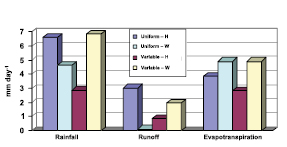
Figure 7.1. Rainfall, runoff and evapotranspiration derived from climate simulation results of Hahmann (H; 2004 ) and Wang and Eltahir (W; 2000 ). Hahmann’s results are for the Amazon centred on the equator, and Wang and Eltahir’s for Africa at the equator. Both studies examined the differences between ‘uniform’ precipitation over a model grid square and ‘variable’ precipitation (added to about 10% of the grid square). Large differences are seen between the two cases in the two studies: a large reduction in precipitation is seen in the Hahmann variable case relative to the uniform case, whereas an increase is seen for the Wang and Eltahir variable case. The differences are even greater for runoff: Hahmann’s uniform case runoff is three times as large as the variable case, whereas Wang and Eltahir have almost no runoff for their uniform case.
7.2.3 Observational Basis for the Effects of Land Surface on Climate
7.2.3.1 Vegetative Controls on Soil Water and its Return Flux to the Atmosphere
Scanlon et al. 2005 [JoC] ) provide an example of how soil moisture can depend on vegetation. They monitored soil moisture in the Nevada desert with lysimeters either including or excluding vegetation and for a multi-year period that included times of anomalously strong precipitation. Without vegetation, much of the moisture penetrated deeply, had a long lifetime and became available for recharge of deep groundwater, whereas for the vegetated plot, the soil moisture was all transpired. In the absence of leaves, forests in early spring also appear as especially dry surfaces with consequent large sensible fluxes that mix the atmosphere to a great depth (e.g., Betts et al., 2001 [JoC] ). Increased water fluxes with spring green-up are observed in terms of a reduction in temperature. Trees in the Amazon can have the largest water fluxes in the dry season by development of deep roots ( (Da Rocha et al., 2004; ) ( Quesada et al., 2004 ) ). Forests can also retard fluxes through control by their leaves. Such control by vegetation of water fluxes is most pronounced for taller or sparser vegetation in cooler or drier climates, and from leaves that are sparse or exert the strongest resistance to water movement. The boreal forest, in particular, has been characterised as a ‘green desert’ because of its small release of water to the atmosphere ( (Gamon et al., 2003 ) ).
7.2.3.2 Land Feedback to Precipitation
Findell and Eltahir 2003 [JoC] ) examine the correlation between early morning near-surface humidity over the USA and an index of the likelihood of precipitation occurrence. They identify different geographical regions with positive, negative or little correlation. Koster et al. 2003 [JoC, ARC] and Koster and Suarez 2004 [JoC, ARC] ) show during summer over the USA, and all land 30°N to 60°N, respectively, a significant correlation of monthly precipitation with that of prior months. They further show that their model only reproduces this correlation if soil moisture feedback is allowed to affect precipitation. Additional observational evidence for such feedback is noted by D’Odorico and Porporato 2004 [JoC] ) in support of a simplified model of precipitation soil moisture coupling (see, e.g., ( Salvucci et al., 2002, ) for support of the null hypothesis of no coupling). Liebmann and Marengo 2001 [JoC] ) point out that the interannual variation of precipitation over the Amazon is largely controlled by the timing of the onset and end of the rainy season. Li and Fu 2004 [JoC] ) provide evidence that onset time of the rainy season is strongly dependent on transpiration by vegetation during the dry season. Previous modelling and observational studies have also suggested that Amazon deforestation should lead to a longer dry season. ( Fu and Li 2004 ) ) further argue from observations that removal of tropical forest reduces surface moisture fluxes, and that such land use changes should contribute to a lengthening of the Amazon dry season. ( Durieux et al. 2003 ) ) find more rainfall in the deforested area in the wet season and a reduction of the dry season precipitation over deforested regions compared with forested areas. Negri et al. 2004 [JoC, ARC] ) obtain an opposite result (although their result is consistent with Durieux during the wet season).
Albedo (the fraction of reflected solar radiation) and emissivity (the ratio of thermal radiation to that of a black body) are important variables for the radiative balance. Surfaces that have more or taller vegetation are commonly darker than are those with sparse or shorter vegetation. With sparse vegetation, the net surface albedo also depends on the albedo of the underlying surfaces, especially if snow or a light-coloured soil. A large-scale transformation of tundra to shrubs, possibly connected to warmer temperatures over the last few decades, has been observed (e.g., Chapin et al., 2005 [JoC] Sturm et al. 2005 [JoC] ) report on winter and melt season observations of how varying extents of such shrubs can modify surface albedo. New satellite data show the importance of radiation heterogeneities at the plot scale for the determination of albedo and the solar radiation used for photosynthesis, and appropriate modelling concepts to incorporate the new data are being advanced (e.g., Yang and Friedl, 2003 [JoC, MoS] ; Niu and Yang, 2004 [JoC] ; Wang, 2005 [MoS] ; Pinty et al., 2006 [JoC, MoS] ).
7.2.3.4 Improved Global and Regional Data
Specification of land surface properties has improved through new, more accurate global satellite observations. In particular, satellite observations have provided albedos of soils in non-vegetated regions (e.g., Tsvetsinskaya et al., 2002 [JoC] ;( Ogawa and Schmugge, 2004; ) Z. Wang, et al., 2004 [Ambiguous] ; Zhou et al., 2005 [JoC, SRC] ) and their emissivities ( Zhou et al., 2003a [JoC, MoS, SRC] ,b). They also constrain model-calculated albedos in the presence of vegetation ( Oleson et al., 2003 [JoC, MoS] ) and vegetation underlain by snow ( Jin et al., 2002 [NPR, JoC] ), and help to define the influence of leaf area on albedo ( Tian et al., 2004 [NPR, JoC, MoS, SRC] ). Precipitation data sets combining rain gauge and satellite observations ( Chen et al., 2002 [JoC] ; Adler et al., 2003 [JoC, ARC] ) are providing diagnostic constraints for climate modelling, as are observations of runoff ( Dai and Trenberth, 2002 [PoC, JoC, MoS, SRC] ; Fekete et al., 2002 [NPR, JoC, MoS] ).
New and improved local site observational constraints collectively describe the land processes that need to be modelled. The largest recent such activity has been the Large-Scale Biosphere-Atmosphere Experiment in Amazonia (LBA) project ( Malhi et al., 2002 [SRC] ; Silva Dias et al., 2002 [JoC] ). Studies within LBA have included physical climate at all scales, carbon and nutrient dynamics and trace gas fluxes. The physical climate aspects are reviewed here. Goncalves et al. 2004 [MoS] ) discuss the importance of incorporating land cover heterogeneity. ( da Rocha et al. 2004 ) ( and Quesada et al. 2004 ) ) quantify water and energy budgets for a forested and a savannah site, respectively. Dry season evapotranspiration for the savannah averaged 1.6 mm day–1 compared with 4.9 mm day–1 for the forest. Both ecosystems depend on deep rooting to sustain evapotranspiration during the dry season, which may help control the length of the dry season (see, e.g., Section 7.2.3.2 ( da Rocha et al. 2004 ) ) also observed that hydraulic lift recharged the forest upper soil profiles each night. At Tapajós, the forest showed no signs of drought stress allowing uniformly high carbon uptake throughout the dry season (July through December 2000; ( da Rocha et al., 2004; ) ( Goulden et al., 2004 ) ). Tibet, another key region, continues to be better characterised from observational studies (e.g., Gao et al., 2004 [JoC, MoS] ; Hong et al., 2004 [JoC] ). With its high elevation, hence low air densities, heating of the atmosphere by land mixes air to a much higher altitude than elsewhere, with implications for vertical exchange of energy. However, the daytime water vapour mixing ratio in this region decreases rapidly with increasing altitude ( Yang et al., 2004 [MoS] ), indicating a strong insertion of dry air from above or by lateral transport.
7.2.3.6 Connecting Changing Vegetation to Changing Climate
Only large-scale patterns are assessed here. Analysis of satellite-sensed vegetation greenness and meteorological station data suggest an enhanced plant growth and lengthened growing season duration at northern high latitudes since the 1980 s ( Zhou et al., 2001 [JoC, SRC] , 2003c ). This effect is further supported by modelling linked to observed climate data ( Lucht et al., 2002 [JoC] Nemani et al. 2002 [JoC] , 2003 ) suggest that increased rainfall and humidity spurred plant growth in the USA and that climate changes may have eased several critical climatic constraints to plant growth and thus increased terrestrial net primary production.
Box 7.1 provides a general description of water fluxes from surface to atmosphere. The most important factors affected by vegetation are soil water availability, leaf area and surface roughness. Whether water has been intercepted on the surface of the leaves or its loss is only from the leaf interior as controlled by stomata makes a large difference. Shorter vegetation with more leaves has the most latent heat flux and the least sensible flux. Replacement of forests with shorter vegetation together with the normally assumed higher albedo could then cool the surface. However, if the replacement vegetation has much less foliage or cannot access soil water as successfully, a warming may occur. Thus, deforestation can modify surface temperatures by up to several degrees celsius in either direction depending on what type of vegetation replaces the forest and the climate regime. Drier air can increase evapotranspiration, but leaves may decrease their stomatal conductance to counter this effect.
7.2.4 Modelling the Coupling of Vegetation, Moisture Availability, Precipitation and Surface Temperature
7.2.4.2 Feedbacks Demonstrated Through Simple Models
In semi-arid systems, the occurrence and amounts of precipitation can be highly variable from year to year. Are there mechanisms whereby the growth of vegetation in times of adequate precipitation can act to maintain the precipitation? Various analyses with simple models have demonstrated how this might happen ( Zeng et al., 2002 [JoC] ;( Foley et al., 2003; ) G. Wang, et al., 2004 [Ambiguous] ; X. Zeng et al., 2004 [Ambiguous] ). Such models demonstrate how assumed feedbacks between precipitation and surface fluxes generated by dynamic vegetation may lead to the possibility of transitions between multiple equilibria for two soil moisture and precipitation regimes. That is, the extraction of water by roots and shading of soil by plants can increase precipitation and maintain the vegetation, but if the vegetation is removed, it may not be able to be restored for a long period. The Sahel region between the deserts of North Africa and the African equatorial forests appears to most readily generate such an alternating precipitation regime.
experiments and find that changes in roughness, soil depth, vegetation cover, stomatal resistance, albedo and leaf area index all could make significant contributions. Voldoire and Royer 2004 [JoC] ) find that such changes may affect temperature and precipitation extremes more than means, in particular the daytime maximum temperature and the drying and temperature responses associated with El Niño events. Guillevic et al. 2002 [JoC] ) address the importance of interannual leaf area variability as inferred from Advanced Very High Resolution Radiometer (AVHRR) satellite data, and infer a sensitivity of climate to this variation. In contrast, Lawrence and Slingo 2004 [NPR, JoC, ARC] ) find little difference in climate simulations that use annual mean vegetation characteristics compared with those that use a prescribed seasonal cycle. However, they do suggest model modifications that would give a much larger sensitivity. Osborne et al. 2004 [JoC] ) examine effects of changing tropical soils and vegetation: variations in vegetation produce variability in surface fluxes and their coupling to precipitation. Thus, interactive vegetation can promote additional variability of surface temperature and precipitation as analysed by Crucifix et al. 2005 [JoC, MoS, SRC] Marengo and Nobre 2001 [NPR] ) found that removal of vegetation led to a decrease in precipitation and evapotranspiration and a decrease in moisture convergence in central and northern Amazonia. Oyama and Nobre 2004 [JoC, MoS] ) show that removal of vegetation in northeast Brazil would substantially decrease precipitation.
7.2.4.3 Consequences of Changing Moisture Availability and Land Cover
Soil moisture control of the partitioning of energy between sensible and latent heat flux is very important for local and
regional temperatures, and possibly their coupling to precipitation. Oglesby et al. 2002 [JoC, MoS] ) carried out a study starting with dry soil where the dryness of the soil over the US Great Plains for at least the first several summer months of their integration produced a warming of about 10°C to 20°C. Williamson et al. 2005 [JoC, MoS] ), have shown that flaws in model formulation of thunderstorms can cause excessive evapotranspiration that lowers temperatures by more than 1°C. Many modelling studies have demonstrated that changing land cover can have local and regional climate impacts that are comparable in magnitude to temperature and precipitation changes observed over the last several decades as reported in Chapter3 .However, since such regional changes can be of both signs, the global average impact is expected to be small. Current literature has large disparities in conclusions. For example, Snyder et al. 2004 [JoC] ) found that removal of northern temperate forests gave a summer warming of 1.3°C and a reduction in precipitation of 1.5 mm day-1.Conversely, Oleson et al. 2004 [JoC, MoS, SRC] ) found that removal of temperate forests in the USA would cool summer temperatures by 0.4°C to 1.5°C and probably increase precipitation, depending on the details of the model and prescription of vegetation. The discrepancy between these two studies may be largely an artefact of different assumptions. The first study assumes conversion of forest to desert and the second to crops. Such studies collectively demonstrate a potentially important impact of human activities on climate through land use modification.
Other recent such studies illustrate various aspects of this issue. Maynard and Royer 2004 [NPR, JoC, MoS] ) address the sensitivity to different parameter changes in African deforestation
7.2.4.4 Mechanisms for Modification of Precipitation by Spatial Heterogeneity
Clark et al. 2004 [MoS, SRC] ) show an example of a ‘squall-line’ simulation where soil moisture variation at the scale of the rainfall modifies the rainfall pattern. Pielke 2001 [JoC, MoS] Weaver et al. 2002 [JoC, MoS] ) and S. Roy et al. 2003 [Ambiguous] ) also address various aspects of small-scale precipitation coupling to land surface heterogeneity. If deforestation occurs in patches rather than uniformly, the consequences for precipitation could be different. Avissar et al. 2002 [JoC, MoS] and Silva Dias et al. 2002 [JoC] ) suggest that there may be a small increase in precipitation (of the order of 10%) resulting from partial deforestation as a consequence of the mesoscale circulations triggered by the deforestation.
Prognostic approaches estimate leaf cover based on physiological processes (e.g., Arora and Boer, 2005 [MoS, SRC] Levis and Bonan 2004 [JoC, MoS, SRC] ) discuss how spring leaf emergence in mid-latitude forests provides a negative feedback to rapid increases in temperature. The parametrization of water uptake by roots contributes to the computed soil water profile ( Feddes et al., 2001 [JoC, MoS] ; Barlage and Zeng, 2004 [JoC, MoS] ), and efforts are being made to make the roots interactive (e.g., Arora and Boer, 2003 [MoS, SRC] ). Dynamic vegetation models have advanced and now explicitly simulate competition between plant functional types (e.g., Bonan et al., 2003 [MoS, SRC] ; Sitch et al., 2003 [MoS] ; Arora and Boer, 2006 [MoS, SRC] ). New coupled climate-carbon models ( Betts et al., 2004 [Ambiguous] ; Huntingford et al., 2004 [MoS] ) demonstrate the possibility of large feedbacks between future climate change and vegetation change, discussed further in Section 7.3.5 (i.e., a die back of Amazon vegetation and reductions in Amazon precipitation). They also indicate that the physiological forcing of stomatal closure by rising atmospheric CO2 levels could contribute 20% to the rainfall reduction. Levis et al. 2004 [Ambiguous] ) demonstrate how African rainfall and dynamic vegetation could change each other.
7.2.5 Evaluation of Models Through Intercomparison
Intercomparison of vegetation models usually involves comparing surface fluxes and their feedbacks. Henderson-Sellers et al. 2003 [JoC, MoS, SRC] ), in comparing the surface fluxes among 20 models, report over an order of magnitude range among sensible fluxes of different models. However, recently developed models cluster more tightly. Irannejad et al. 2003 [JoC, MoS, SRC] ) developed a statistical methodology to fit monthly fluxes from a large number of climate models to a simple linear statistical model, depending on factors such as monthly net radiation and surface relative humidity. Both the land and atmosphere models are major sources of uncertainty for feedbacks. Irannejad et al. find that coupled models agree more closely due to offsetting differences in the atmospheric and land models. Modelling studies have long reported that soil moisture can influence precipitation. Only recently, however, have there been attempts to quantify this coupling from a statistical viewpoint ( Dirmeyer, 2001 [JoC, ARC] ; Koster and Suarez, 2001 [JoC, MoS, ARC] ; Koster et al., 2002 [JoC, MoS, ARC] ; Reale and Dirmeyer, 2002 [JoC, MoS, ARC] ; Reale et al., 2002 [JoC, MoS, ARC] ; Koster et al., 2003 [JoC, ARC] ; Koster and Suarez, 2004 [JoC, ARC] Koster et al. 2004 [JoC, ARC] , 2006 and Guo et al. 2006 [JoC] ) report on a new model intercomparison activity, the Global Land Atmosphere Coupling Experiment (GLACE), which compares among climate models differences in precipitation variability caused by interaction with soil moisture. Using an experimental protocol to generate ensembles of simulations with soil moisture that is either prescribed or interactive as it evolves in time, they report a wide range of differences between models( Figure 7.2 Lawrence and Slingo 2005 [JoC, ARC] ) show that the relatively weak coupling strength of the Hadley Centre model results from its atmospheric component. There is yet little confidence in this feedback component of climate models and therefore its possible contribution to global warming (see Chapter8 ).
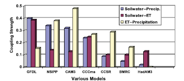
Figure 7.2. Coupling strength (a nondimensional pattern similarity diagnostic defined in Koster et al., 2006 [JoC, ARC] ) between summer rainfall and soil water in models assessed by the GLACE study ( Guo et al., 2006 [JoC] ), divided into how strongly soil water causes evaporation (including from plants) and how strongly this evaporation causes rainfall. The soil water-precipitation coupling is scaled up by a factor of 10, and the two indices for evaporation to precipitation coupling given in the study are averaged. Models include the Geophysical Fluid Dynamics Laboratory (GFDL) model, the National Aeronautics and Space Administration (NASA) Seasonal to Interannual Prediction Program (NSIPP) model, the National Center for Atmospheric Research Community Atmosphere Model (CAM3), the Canadian Centre for Climate Modelling and Analysis (CCCma) model, the Centre for Climate System Research (CCSR) model, the Bureau of Meteorology Research Centre (BMRC) model and the Hadley Centre Atmospheric Model version 3 (HadAM3).
7.2.6 Linking Biophysical to Biogeochemical and Ecohydrological Components
Soil moisture and surface temperatures work together in response to precipitation and radiative inputs. Vegetation influences these terms through its controls on energy and water fluxes, and through these fluxes, precipitation. It also affects the radiative heating. Clouds and precipitation are affected through modifications of the temperature and water vapour content of near-surface air. How the feedbacks of land to the atmosphere work remains difficult to quantify from either observations or modelling (as addressed in Sections 7.2.3.2 and 7.2.5.1). Radiation feedbacks depend on vegetation or cloud cover that has changed because of changing surface temperatures or moisture conditions. How such conditions may promote or discourage the growth of vegetation is established by various ecological studies. The question of how vegetation will change its distribution at large scales and the consequent changes in absorbed radiation is quantified through remote sensing studies. At desert margins, radiation and precipitation feedbacks may act jointly with vegetation. Radiation feedbacks connected to vegetation may be most pronounced at the margins between boreal forests and tundra and involve changes in the timing of snowmelt. How energy is transferred from the vegetation to underlying snow surfaces is understood in general terms but remains problematic in modelling and process details. Dynamic vegetation models (see Section 7.2.4.5 )synthesize current understanding.
Changing soil temperatures and snow cover affect soil microbiota and their processing of soil organic matter. How are nutrient supplies modified by these surface changes or delivery from the atmosphere? In particular, the treatment of carbon fluxes (addressed in more detail in Section 7.3 )may require comparable or more detail in the treatment of N cycling (as attempted by S. Wang, et al., 2002 [JoC, MoS] ; Dickinson et al., 2003 [MoS, SRC] ). The challenge is to establish better process understanding at local scales and appropriately incorporate this understanding into global models. The Coupled Carbon-Cycle Climate Model Intercomparison Project (C4MIP) simulations described in Section 7.3.5 are a first such effort.
Biomass burning is a major mechanism for changing vegetation cover and generation of atmospheric aerosols and is directly coupled to the land climate variables of moisture and near-surface winds, as addressed for the tropics by Hoffman et al. 2002 [NPR, JoC] ). The aerosol plume produced by biomass burning at the end of the dry season contains black carbon that absorbs radiation. The combination of a cooler surface due to lack of solar radiation and a warmer boundary layer due to absorption of solar radiation increases the thermal stability and reduces cloud formation, and thus can reduce rainfall. ( Freitas et al. 2005 ) ) indicate the possibility of rainfall decrease in the Plata Basin as a response to the radiative effect of the aerosol load transported from biomass burning in the Cerrado and Amazon regions. Aerosols and clouds reduce the availability of visible light needed by plants for photosynthesis. However, leaves in full sun may be light saturated, that is, they do not develop sufficient enzymes to utilise that level of light. Leaves that are shaded, however, are generally light limited. They are only illuminated by diffuse light scattered by overlying leaves or by atmospheric constituents. Thus, an increase in diffuse light at the expense of direct light may promote leaf carbon assimilation and transpiration ( (Roderick et al., 2001; ) Cohan et al., 2002 [JoC] ; Gu et al., 2002 [JoC] , 2003 ( Yamasoe et al. 2006 ) ) report the first observational tower evidence for this effect in the tropics. Diffuse radiation resulting from the Mt. Pinatubo eruption may have created an enhanced terrestrial carbon sink ( (Roderick et al., 2001; ) Gu et al., 2003 [JoC] Angert et al. 2004 [JoC] ) provide an analysis that rejects this hypothesis relative to other possible mechanisms.
7.3 The Carbon Cycle and the Climate System
7.3.1 Overview of the Global Carbon Cycle
7.3.1.1 The Natural Carbon Cycle
Over millions of years, CO2 is removed from the atmosphere through weathering by silicate rocks and through burial in marine sediments of carbon fixed by marine plants (e.g., ( Berner, 1998 ) ). Burning fossil fuels returns carbon captured by plants in Earth’s geological history to the atmosphere. New ice core records show that the Earth system has not experienced current atmospheric concentrations of CO2,or indeed of CH4,for at least 650 kyr – six glacial-interglacial cycles. During that period the atmospheric CO2 concentration remained between 180 ppm (glacial maxima) and 300 ppm (warm interglacial periods) ( Siegenthaler et al., 2005 [JoC] ). It is generally accepted that during glacial maxima, the CO2 removed from the atmosphere was stored in the ocean. Several causal mechanisms have been identified that connect astronomical changes, climate, CO2 and other greenhouse gases, ocean circulation and temperature, biological productivity and nutrient supply, and interaction with ocean sediments (see Box 6.2 ).
Prior to 1750, the atmospheric concentration of CO2 had been relatively stable between 260 and 280 ppm for 10 kyr( Box 6.2 ). Perturbations of the carbon cycle from human activities were insignificant relative to natural variability. Since 1750, the concentration of CO2 in the atmosphere has risen, at an increasing rate, from around 280 ppm to nearly 380 ppm in 2005 (see Figure 2.3 and FAQ 2.1 ,Figure 1). The increase in atmospheric CO2 concentration results from human activities: primarily burning of fossil fuels and deforestation, but also cement production and other changes in land use and management such as biomass burning, crop production and conversion of grasslands to croplands (see FAQ 7.1 ). While human activities contribute to climate change in many direct and indirect ways, CO2 emissions from human activities are considered the single largest anthropogenic factor contributing to climate change (see FAQ 2.1 ,Figure 2). Atmospheric CH4 concentrations have similarly experienced a rapid rise from about 700 ppb in 1750 ( Flückiger et al., 2002 [NPR, JoC] ) to about 1,775 ppb in 2005 (see Section 2.3.2 ): sources include fossil fuels, landfills and waste treatment, peatlands/wetlands, ruminant animals and rice paddies. The increase in CH4 radiative forcing is slightly less than one-third that of CO2,making it the second most important greenhouse gas (see Chapter2 ). The CH4 cycle is presented in Section 7.4.1 .
Both CO2 and CH4 play roles in the natural cycle of carbon, involving continuous flows of large amounts of carbon among the ocean, the terrestrial biosphere and the atmosphere, that maintained stable atmospheric concentrations of these gases for 10 kyr prior to 1750 . Carbon is converted to plant biomass by photosynthesis. Terrestrial plants capture CO2 from the atmosphere; plant, soil and animal respiration (including decomposition of dead biomass) returns carbon to the atmosphere as CO2,or as CH4 under anaerobic conditions. Vegetation fires can be a significant source of CO2 and CH4 to the atmosphere on annual time scales, but much of the CO2 is recaptured by the terrestrial biosphere on decadal time scales if the vegetation regrows.
Carbon dioxide is continuously exchanged between the atmosphere and the ocean. Carbon dioxide entering the surface ocean immediately reacts with water to form bicarbonate (HCO3–)and carbonate (CO32–)ions. Carbon dioxide, HCO3– and CO32– are collectively known as dissolved inorganic carbon (DIC). The residence time of CO2 (as DIC) in the surface ocean, relative to exchange with the atmosphere and physical exchange with the intermediate layers of the ocean below, is less than a decade. In winter, cold waters at high latitudes, heavy and enriched with CO2 (as DIC) because of their high solubility, sink from the surface layer to the depths of the ocean. This localised sinking, associated with the Meridional Overturning Circulation (MOC; Box 5.1 )is termed the ‘solubility pump’. Over time, it is roughly balanced by a distributed diffuse upward transport of DIC primarily into warm surface waters.
Phytoplankton take up carbon through photosynthesis. Some of that sinks from the surface layer as dead organisms and particles (the ‘biological pump’), or is transformed into dissolved organic carbon (DOC). Most of the carbon in sinking particles is respired (through the action of bacteria) in the surface and intermediate layers and is eventually recirculated to the surface as DIC. The remaining particle flux reaches abyssal depths and a small fraction reaches the deep ocean sediments, some of which is re-suspended and some of which is buried. Intermediate waters mix on a time scale of decades to centuries, while deep waters mix on millennial time scales. Several mixing times are required to bring the full buffering capacity of the ocean into effect (see Section 5.4 for long-term observations of the ocean carbon cycle and their consistency with ocean physics).
Together the solubility and biological pumps maintain a vertical gradient in CO2 (as DIC) between the surface ocean (low) and the deeper ocean layers (high), and hence regulate exchange of CO2 between the atmosphere and the ocean. The strength of the solubility pump depends globally on the strength of the MOC, surface ocean temperature, salinity, stratification and ice cover. The efficiency of the biological pump depends on the fraction of photosynthesis exported from the surface ocean as sinking particles, which can be affected by changes in ocean circulation, nutrient supply and plankton community composition and physiology.
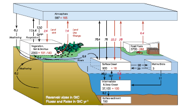
Figure 7.3. The global carbon cycle for the 1990 s, showing the main annual fluxes in GtC yr–1:pre-industrial ‘natural’ fluxes in black and ‘anthropogenic’ fluxes in red (modified from Sarmiento and Gruber, 2006 [NPR, SRC] , with changes in pool sizes from Sabine et al., 2004a [JoC, SRC] ). The net terrestrial loss of –39 GtC is inferred from cumulative fossil fuel emissions minus atmospheric increase minus ocean storage. The loss of –140 GtC from the ‘vegetation, soil and detritus’ compartment represents the cumulative emissions from land use change ( Houghton, 2003 [JoC, MoS] ), and requires a terrestrial biosphere sink of 101 GtC (in Sabine et al., given only as ranges of –140 to –80 GtC and 61 to 141 GtC, respectively; other uncertainties given in their Table 1). Net anthropogenic exchanges with the atmosphere are from Column 5 ‘AR4’ in Table 7.1 .Gross fluxes generally have uncertainties of more than ±20% but fractional amounts have been retained to achieve overall balance when including estimates in fractions of GtC yr–1 for riverine transport, weathering, deep ocean burial, etc. ‘GPP’ is annual gross (terrestrial) primary production. Atmospheric carbon content and all cumulative fluxes since 1750 are as of end 1994 .
In Figure 7.3 the natural or unperturbed exchanges (estimated to be those prior to 1750 ) among oceans, atmosphere and land are shown by the black arrows. The gross natural fluxes between the terrestrial biosphere and the atmosphere and between the oceans and the atmosphere are (circa 1995 ) about 120 and 90 GtC yr–1,respectively. Just under 1 GtC yr–1 of carbon is transported from the land to the oceans via rivers either dissolved or as suspended particles (e.g., Richey, 2004 [NPR] ). While these fluxes vary from year to year, they are approximately in balance when averaged over longer time periods. Additional small natural fluxes that are important on longer geological time scales include conversion of labile organic matter from terrestrial plants into inert organic carbon in soils, rock weathering and sediment accumulation (‘reverse weathering’), and release from volcanic activity. The net fluxes in the 10 kyr prior to 1750, when averaged over decades or longer, are assumed to have been less than about 0.1 GtC yr–1.For more background on the carbon cycle, see Prentice et al. 2001 [NPR] Field and Raupach 2004 [NPR, SRC] and Sarmiento and Gruber 2006 [NPR, SRC] ).
7.3.1.2 Perturbations of the Natural Carbon Cycle from Human Activities
The additional burden of CO2 added to the atmosphere by human activities, often referred to as ‘anthropogenic CO2’ leads to the current ‘perturbed’ global carbon cycle. Figure 7.3 shows that these ‘anthropogenic emissions’ consist of two fractions: (i) CO2 from fossil fuel burning and cement production, newly released from hundreds of millions of years of geological storage (see Section 2.3 )and (ii) CO2 from deforestation and agricultural development, which has been stored for decades to centuries. Mass balance estimates and studies with other gases indicate that the net land-atmosphere and ocean-atmosphere fluxes have become significantly different from zero, as indicated by the red arrows in Figure 7.3 (see also Section 7.3.2 ). Although the anthropogenic fluxes of CO2 between the atmosphere and both the land and ocean are just a few percent of the gross natural fluxes, they have resulted in measurable changes in the carbon content of the reservoirs since pre-industrial times as shown in red. These perturbations to the natural carbon cycle are the dominant driver of climate change because of their persistent effect on the atmosphere. Consistent with the response function to a CO2 pulse from the Bern Carbon Cycle Model (see footnote (a) of Table 2.14 ), about 50% of an increase in atmospheric CO2 will be removed within 30 years, a further 30% will be removed within a few centuries and the remaining 20% may remain in the atmosphere for many thousands of years ( Prentice et al., 2001 [NPR] ; Archer, 2005 [JoC, SRC] ; see also Sections 7.3.4.2 and 10.4 )
About 80% of anthropogenic CO2 emissions during the 1990 s resulted from fossil fuel burning, with about 20% from land use change (primarily deforestation)( Table 7.1 ). Almost 45% of combined anthropogenic CO2 emissions (fossil fuel plus land use) have remained in the atmosphere. Oceans are estimated to have taken up approximately 30% (about 118 ± 19 GtC: Sabine et al., 2004a [JoC, SRC] ; Figure 7.3 ), an amount that can be accounted for by increased atmospheric concentration of CO2 without any change in ocean circulation or biology. Terrestrial ecosystems have taken up the rest through growth of replacement vegetation on cleared land, land management practices and the fertilizing effects of elevated CO2 and N deposition (see Section 7.3.3 ).
Because CO2 does not limit photosynthesis significantly in the ocean, the biological pump does not take up and store anthropogenic carbon directly. Rather, marine biological cycling of carbon may undergo changes due to high CO2 concentrations, via feedbacks in response to a changing climate. The speed with which anthropogenic CO2 is taken up effectively by the ocean, however, depends on how quickly surface waters are transported and mixed into the intermediate and deep layers of the ocean. A considerable amount of anthropogenic CO2 can be buffered or neutralized by dissolution of CaCO3 from surface sediments in the deep sea, but this process requires many thousands of years.
The increase in the atmospheric CO2 concentration relative to the emissions from fossil fuels and cement production only is defined here as the ‘airborne fraction’. [2] Land emissions, although significant, are not included in this definition due to the difficulty of quantifying their contribution, and to the complication that much land emission from logging and clearing of forests may be compensated a few years later by uptake associated with regrowth. The ‘airborne fraction of total emissions’ is thus defined as the atmospheric CO2 increase as a fraction of total anthropogenic CO2 emissions, including the net land use fluxes. The airborne fraction varies from year to year mainly due to the effect of interannual variability in land uptake (see Section 7.3.2 ).
7.3.1.3 New Developments in Knowledge of the Carbon Cycle Since the Third Assessment Report
Sections 7.3.2 to 7.3.5 describe where knowledge and understanding have advanced significantly since the Third Assessment Report (TAR). In particular, the budget of anthropogenic CO2 (shown by the red fluxes in Figure 7.3 )can be calculated with improved accuracy. In the ocean, newly available high-quality data on the ocean carbon system have been used to construct robust estimates of the cumulative ocean burden of anthropogenic carbon ( Sabine et al., 2004a [JoC, SRC] ) and associated changes in the carbonate system ( Feely et al., 2004 [JoC, ARC] ). The pH in the surface ocean is decreasing, indicating the need to understand both its interaction with a changing climate and the potential impact on organisms in the ocean (e.g., Orr et al., 2005 [JoC, ARC] ; Royal Society, 2005 [NPR] ). On land, there is a better understanding of the contribution to the buildup of CO2 in the atmosphere since 1750 associated with land use and of how the land surface and the terrestrial biosphere interact with a changing climate. Globally, inverse techniques used to infer the magnitude and location of major fluxes in the global carbon cycle have continued to mature, reflecting both refinement of the techniques and the availability of new observations. During preparation of the TAR, inclusion of the carbon cycle in climate models was new. Now, results from the firstC4MIP are available: when the carbon cycle is included, the models consistently simulate climate feedbacks to land and ocean carbon cycles that tend to reduce uptake of CO2 by land and ocean from 1850 to 2100 (see Section 7.3.5 ).
Table 7.2. Land to atmosphere emissions resulting from land use changes during the 1990 s and the 1980 s (GtC yr–1). The Fourth Assessment Report (AR4) estimates used in the global carbon budget (Table 7.1) are shown in bold. Positive values indicate carbon losses from land ecosystems. Uncertainties are reported as ±1 standard deviation. Numbers in parentheses are ranges of uncertainty.
| Tropical Americas | Tropical Africa | Tropical Asia | Pan-Tropical | Non-tropics | Total Globe | |
|---|---|---|---|---|---|---|
| 1990s | ||||||
| Houghton (2003a)a | 0.8 ± 0.3 | 0.4 ± 0.2 | 1.1 ± 0.5 | 2.2 ± 0.6 | –0.02 ± 0.5 | 2.2 ± 0.8 |
| DeFries et al. (2002)b | 0.5 (0.2 to 0.7) | 0.1 (0.1 to 0.2) | 0.4 (0.2 to 0.6) | 1.0 (0.5 to 1.6) | n.a. | n.a. |
| Achard et al. (2004)c | 0.3 (0.3 to 0.4) | 0.2 (0.1 to 0.2) | 0.4 (0.3 to 0.5) | 0.9 (0.5 to 1.4) | n.a. | n.a. |
| AR4d | 0.7 (0.4 to 0.9) | 0.3 (0.2 to 0.4) | 0.8 (0.4 to 1.1) | 1.6 (1.0 to 2.2) | –0.02 (–0.5 to +0.5) | 1.6 (0.5 to 2.7) |
| 1980s | ||||||
| Houghton (2003a)a | 0.8 ± 0.3 | 0.3 ± 0.2 | 0.9 ± 0.5 | 1.9 ± 0.6 | 0.06 ± 0.5 | 2.0 ± 0.8 |
| DeFries et al. (2002)b | 0.4 (0.2 to 0.5) | 0.1 (0.08 to 0.14) | 0.2 (0.1 to 0.3) | 0.7 (0.4 to 1.0) | n.a. | n.a. |
| McGuire et al. (2001)e | 0.6 to 1.2 | –0.1 to +0.4 | (0.6 to 1.0) | |||
| Jain and Yang (2005)f | 0.22 to 0.24 | 0.08 to 0.48 | 0.58 to 0.34 | - | - | 1.33 to 2.06 |
| TARg | 1.7 (0.6 to 2.5) | |||||
| AR4d | 0.6 (0.3 to 0.8) | 0.2 (0.1 to 0.3) | 0.6 (0.3 to 0.9) | 1.3 (0.9 to 1.8) | 0.06 (–0.4 to +0.6) | 1.4 (0.4 to 2.3) |
Notes:
a His Table 2.
b Their Table 3.
c Their Table 2 for mean estimates with the range indicated in parentheses corresponding to their reported minimum and maximum estimates.
d Best estimate calculated from the mean of Houghton 2003a [JoC, MoS] ) and DeFries et al. ( 2002 ), the only two studies covering both the 1980 s and the 1990 s. For non-tropical regions where DeFries et al. have no estimate, Houghton has been used.
e Their Table 5; range is obtained from four terrestrial carbon models.
f The range indicated in parentheses corresponds to two simulations using the same model, but forced with different land cover change datasets from Houghton 2003a [JoC, MoS] ) and DeFries et al. ( 2002 ).
g In the TAR estimate, no values were available for the 1990 s.
7.3.2 The Contemporary Carbon Budget
7.3.2.1 Atmospheric Increase
The atmospheric CO2 increase is measured with great accuracy at various monitoring stations (see Chapter2 ;and Keeling and Whorf, 2005 [NPR, ARC] updated by S. Piper through 2006 ). The mean yearly increase in atmospheric CO2 (the CO2 ‘growth rate’) is reported in Table 7.1 .Atmospheric CO2 has continued to increase since the TAR( Figure 7.4 ), and the rate of increase appears to be higher, with the average annual increment rising from 3.2 ± 0.1 GtC yr–1 in the 1990 s to 4.1 ± 0.1 GtC yr–1 in the period 2000 to 2005 . The annual increase represents the net effect of several processes that regulate global land-atmosphere and ocean-atmosphere fluxes, examined below. The ‘airborne fraction’ (atmospheric increase in CO2 concentration/fossil fuel emissions) provides a basic benchmark for assessing short- and long-term changes in these processes. From 1959 to the present, the airborne fraction has averaged 0.55, with remarkably little variation when block-averaged into five-year bins( Figure 7.4 ). Thus, the terrestrial biosphere and the oceans together have consistently removed 45% of fossil CO2 for the last 45 years, and the recent higher rate of atmospheric CO2 increase largely reflects increased fossil fuel emissions. Year-to-year fluctuations in the airborne fraction are associated with major climatic events (see Section 7.3.2.4 ). The annual increase in 1998, 2.5 ppm, was the highest ever observed, but the airborne fraction (0.82) was no higher than values observed several times in prior decades. The airborne fraction dropped significantly below the average in the early 1990 s, and preliminary data suggest it may have risen above the average in 2000 to 2005 .
Table 7.1. The global carbon budget (GtC yr–1); errors represent ±1 standard deviation uncertainty estimates and not interannual variability, which is larger. The atmospheric increase (first line) results from fluxes to and from the atmosphere: positive fluxes are inputs to the atmosphere (emissions); negative fluxes are losses from the atmosphere (sinks); and numbers in parentheses are ranges. Note that the total sink of anthropogenic CO2 is well constrained. Thus, the ocean-to-atmosphere and land-to-atmosphere fluxes are negatively correlated: if one is larger, the other must be smaller to match the total sink, and vice versa.
| 1980s | 1990s | 2000–2005c | |||
|---|---|---|---|---|---|
| TAR | TAR reviseda | TAR | AR4 | AR4 | |
| Atmospheric Increaseb | 3.3 ± 0.1 | 3.3 ± 0.1 | 3.2 ± 0.1 | 3.2 ± 0.1 | 4.1 ± 0.1 |
| Emissions (fossil + cement)c | 5.4 ± 0.3 | 5.4 ± 0.3 | 6.4 ± 0.4 | 6.4 ± 0.4 | 7.2 ± 0.3 |
| Net ocean-to-atmosphere fluxd | –1.9 ± 0.6 | –1.8 ± 0.8 | –1.7 ± 0.5 | –2.2 ± 0.4 | –2.2 ± 0.5 |
| Net land-to-atmosphere fluxe | –0.2 ± 0.7 | –0.3 ± 0.9 | –1.4 ± 0.7 | –1.0 ± 0.6 | –0.9 ± 0.6 |
| Partitioned as follows | |||||
| Land use change flux | 1.7 (0.6 to 2.5) | 1.4 (0.4 to 2.3) | n.a. | 1.6 (0.5 to 2.7) | n.a. |
| Residual terrestrial sink | –1.9 (–3.8 to –0.3) | –1.7 (–3.4 to 0.2) | n.a. | –2.6 (–4.3 to –0.9) | n.a. |
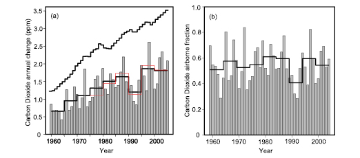
Figure 7.4. Changes in global atmospheric CO2 concentrations. (a) Annual (bars) and five-year mean (lower black line) changes in global CO2 concentrations, from Scripps Institution of Oceanography observations (mean of South Pole and Mauna Loa; Keeling and Whorf, 2005 [NPR, ARC] , updated). The upper stepped line shows annual increases that would occur if 100% of fossil fuel emissions ( Marland et al., 2006 [NPR] , updated as described in Chapter2 )remained in the atmosphere, and the red line shows five-year mean annual increases from National Oceanic and Atmospheric Administration (NOAA) data (mean of Samoa and Mauna Loa; Tans and Conway, 2005 [NPR, ARC] , updated). (b) Fraction of fossil fuel emissions remaining in the atmosphere (‘airborne fraction’) each year (bars), and five-year means (solid black line) (Scripps data) (mean since 1958 is 0.55). Note the anomalously low airborne fraction in the early 1990 s.
The inter-hemispheric gradient of CO2 provides additional evidence that the increase in atmospheric CO2 is caused primarily by NH sources. The excess atmospheric CO2 in the NH compared with the Southern Hemisphere (SH), ΔCO2N-S,has increased in proportion to fossil fuel emission rates (which are predominantly in the NH) at about 0.5 ppm per (GtC yr–1)( Figure 7.5 ). The intercept of the best-fit line indicates that, without anthropogenic emissions, atmospheric CO2 would be 0.8 ppm higher in the SH than in the NH, presumably due to transport of CO2 by the ocean circulation. The consistency of the airborne fraction and the relationship between
ΔCO2N-S and fossil fuel emissions suggest broad consistency in the functioning of the carbon cycle over the period. There are interannual fluctuations in ΔCO2N-S as large as ±0.4 ppm, at least some of which may be attributed to changes in atmospheric circulation ( Dargaville et al., 2000 [JoC, MoS] ), while others may be due to shifts in sources and sinks, such as large forest fires.
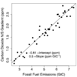
Figure 7.5. The difference between CO2 concentration in the NH and SH (y axis), computed as the difference between annual mean concentrations (ppm) at Mauna Loa and the South Pole ( Keeling and Whorf, 2005 [NPR, ARC] , updated), compared with annual fossil fuel emissions (x axis; GtC; Marland, et al., 2006 [NPR] ), with a line showing the best fit. The observations show that the north-south difference in CO2 increases proportionally with fossil fuel use, verifying the global impact of human-caused emissions.
7.3.2.1.1 Fossil fuel and cement emissions
Fossil fuel and cement emissions rose from 5.4 ± 0.3 GtC yr–1 in the 1980 s to 6.4 ± 0.4 GtC yr–1 in the 1990 s ( Marland et al., 2006 [NPR] ). They have continued to increase between the 1990 s and 2000 to 2005, climbing to 7.2 ± 0.3 GtC yr–1.These numbers are estimated based upon international energy statistics for the 1980 to 2003 period ( Marland et al., 2006 [NPR] ) with extrapolated trends for 2004 to 2005 (see Table 7.1 ). The error (±1 standard deviation) for fossil fuel and cement emissions is of the order of 5% globally. Cement emissions are small compared with fossil fuel emissions (roughly 3% of the total).
7.3.2.1.2 Land use change
During the past two decades, the CO2 flux caused by land use changes has been dominated by tropical deforestation. Agriculture and exploitation of forest resources have reached into formerly remote areas of old growth forest in the tropics, in contrast to mid-latitudes where exploitation previously eliminated most old growth forests. The land use change fluxes reported in this section include explicitly some accumulation of carbon by regrowing vegetation (e.g., Houghton et al., 2000 [JoC] ). In the TAR, the global land use flux, adapted from Houghton 1999 [JoC] ), was estimated to be 1.7 (0.6–2.5) GtC yr–1 for the 1980 s. No estimate was available at the time for the 1990 s. This estimate is based on a ‘bookkeeping’ carbon model prescribed with deforestation statistics ( Houghton, 1999 [JoC] ). A markedly lower estimate of the land use flux in the 1980 s( Table 7.2 )was obtained by McGuire et al. 2001 [JoC, MoS] ) from four process-driven terrestrial carbon models, prescribed with changes in cropland area from Ramankutty and Foley 1999 [JoC, MoS, ARC] ). The higher land use emissions of Houghton 2003a [JoC, MoS] ) may reflect both the additional inclusion of conversion of forest to pasture and the use of a larger cropland expansion rate than the one of Ramankutty and Foley 1999 [JoC, MoS, ARC] ), as noted by Jain and Yang 2005 [NPR, JoC, MoS] Houghton 2003a [JoC, MoS] ) updated the land use flux to 2.0 ± 0.8 GtC yr–1 for the 1980 s and 2.2 ± 0.8 GtC yr–1 for the 1990 s (see Table 7.2 ). This update gives higher carbon losses from tropical deforestation than those in the TAR ( Houghton 2003b [MoS] ).
In addition, DeFries et al. ( 2002 ) estimated a tropical land use flux of 0.7 (0.4–1.0) GtC yr–1 for the 1980 s and 1.0 (0.5–1.6) GtC yr–1 for the 1990 s, using the same bookkeeping approach as Houghton 1999 [JoC] ) but driven by remotely sensed data on deforested areas. A similar estimate was independently produced by Achard et al. 2004 [JoC, MoS] ) for the 1990 s, also based on remote sensing. These different land use emissions estimates are reported in Table 7.2 .Although the two recent satellite-based estimates point to a smaller source than that of Houghton 2003a [JoC, MoS] ), it is premature to say that Houghton’s numbers are overestimated. The land use carbon source has the largest uncertainties in the global carbon budget. If a high value for the land use source is adopted in the global budget, then the residual land uptake over undisturbed ecosystems should be a large sink, and vice versa. For evaluating the global carbon budget, the mean of DeFries et al. ( 2002 and Houghton 2003a [JoC, MoS] ), which both cover the 1980 s and the 1990 s( Table 7.2 ), was chosen and the full range of uncertainty is reported. The fraction of carbon emitted by fossil fuel burning, cement production and land use changes that does not accumulate in the atmosphere must be taken up by land ecosystems and by the oceans.
7.3.2.2 Uptake of CO2 by Natural Reservoirs and Global Carbon Budget
7.3.2.2.1 Ocean-atmosphere flux
To assess the mean ocean sink, seven methods have been used. The methods are based on: (1) observations of the partial pressure of CO2 at the ocean surface and gas-exchange estimates ( (Takahashi et al., 2002 ) ); (2) atmospheric inversions based upon diverse observations of atmospheric CO2 and atmospheric transport modelling (see Section 7.2.3.4 ); (3) observations of carbon, oxygen, nutrients and chlorofluorocarbons (CFCs) in seawater, from which the concentration of anthropogenic CO2 is estimated ( Sabine et al., 2004a [JoC, SRC] ) combined with estimates of oceanic transport ( Gloor et al., 2003 [JoC, MoS] ; Mikaloff Fletcher et al., 2006 [NPR, JoC, MoS] ); (4) estimates of the distribution of water age based on CFC observations combined with the atmospheric CO2 history ( McNeil et al., 2003 [JoC] ); (5) the simultaneous observations of the increase in atmospheric CO2 and decrease in atmosphericO2 ( Manning and Keeling, 2006 [JoC, ARC] ); (6) various methods using observations of change in 13Cin the atmosphere ( Ciais et al., 1995 [JoC, SRC] ) or the oceans ( Gruber and Keeling, 2001 [JoC, MoS, SRC] ; Quay et al., 2003 [JoC] ); and (7) ocean General Circulation Models ( Orr et al., 2001 [JoC, MoS, ARC] ). The ocean uptake estimates obtained with methods (1) and (2) include in part a flux component due to the outgassing of river-supplied inorganic and organic carbon ( Sarmiento and Sundquist, 1992 [JoC] ). The magnitude of this necessary correction to obtain the oceanic uptake flux of anthropogenic CO2 is not well known, as these estimates pertain to the open ocean, whereas a substantial fraction of the river-induced outgassing likely occurs in coastal regions. These estimates of the net oceanic sink are shown in Figure 7.3 .
With these corrections, estimates from all methods are consistent, resulting in a well-constrained global oceanic sink for anthropogenic CO2 (see Table 7.1 ). The uncertainty around the different estimates is more difficult to judge and varies considerably with the method. Four estimates appear better constrained than the others. The estimate for the ocean uptake of atmospheric CO2 of –2.2 ± 0.5 GtC yr–1 centred around 1998 based on the atmosphericO2/N2 ratio needs to be corrected for the oceanicO2 changes ( Manning and Keeling, 2006 [JoC, ARC] ). The estimate of –2.0 ± 0.4 GtC yr–1 centred around 1995 based on CFC observations provides a constraint from observed physical transport in the ocean. These estimates of the ocean sink are shown in Figure 7.6 .The mean estimates of –2.2 ± 0.25 and –2.2 ± 0.2 GtC yr–1 centred around 1995 and 1994 provide constraints based on a large number of ocean carbon observations. These well-constrained estimates all point to a decadal mean ocean CO2 sink of –2.2 ± 0.4 GtC yr–1 centred around 1996, where the uncertainty is the root mean square of all errors. See Section 5.4 for a discussion of changes in the ocean CO2 sink.
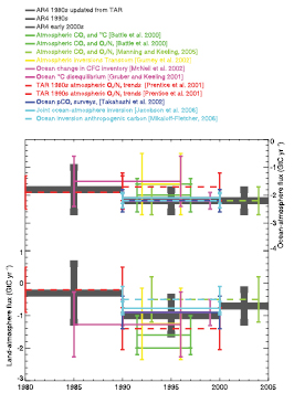
Figure 7.6. Individual estimates of the ocean-atmosphere flux reported in Chapter5 and of the related land-atmosphere flux required to close the global carbon budget. The dark thick lines are the revised budget estimates in the AR4 for the 1980 s, the 1990 s and the early 2000 s, respectively.
7.3.2.2.2 Land-atmosphere flux
The land-atmosphere CO2 flux is the sum of the land use change CO2 flux (see Section 7.3.2.1 )plus sources and sinks due for instance to legacies of prior land use, climate, rising CO2 or N deposition (see Section 7.3.3 for a review of processes). For assessing the global land-atmosphere flux, more than just direct terrestrial observations must be used, because observations of land ecosystem carbon fluxes are too sparse and the ecosystems are too heterogeneous to allow global assessment of the net land flux with sufficient accuracy. For instance, large-scale biomass inventories ( (Goodale et al., 2002; ) UN-ECE/FAO, 2000 ) are limited to forests with commercial value, and they do not adequately survey tropical forests. Direct flux observations by the eddy covariance technique are only available at point locations, most do not yet have long-term coverage and they require considerable upscaling to obtain global estimates ( Baldocchi et al., 2001 [JoC] ). As a result, two methods can be used to quantify the net global land-atmosphere flux: (1) deducing that quantity as a residual between the fossil fuel and cement emissions and the sum of ocean uptake and atmospheric increase( Table 7.1 ), or (2) inferring the land-atmosphere flux simultaneously with the ocean sink by inverse analysis or mass balance computations using atmospheric CO2 data, with terrestrial and marine processes distinguished usingO2/N2 and/or 13Cobservations. Individual estimates of the land-atmosphere flux deduced using either method 1 or method 2 are shown in Figure 7.6 .Method 2 was used in the TAR, based uponO2/N2 data ( Langenfelds et al., 1999 [JoC] ; Battle et al., 2000 [JoC] ). Corrections have been made to the results of method 2 to account for the effects of thermalO2 fluxes by the ocean ( Le Quéré et al., 2003 [JoC, SRC] ). This chapter includes these corrections to update the 1980 s budget, resulting in a land net flux of –0.3 ± 0.9 GtC yr–1 during the 1980 s. For the 1990 s and after, method 1 was adopted for assessing the ocean sink and the land-atmosphere flux. Unlike in the TAR, method 1 is preferred for the 1990 s and thereafter (i.e., estimating first the ocean uptake, and then deducing the land net flux) because the ocean uptake is now more robustly determined by various oceanographic approaches (see 7.3.2.2.1) than by the atmosphericO2 trends. The numbers are reported in Table 7.1 .The land-atmosphere flux evolved from a small sink in the 1980 s of –0.3 ± 0.9 GtC yr–1 to a large sink during the 1990 s of –1.0 ± 0.6 GtC yr–1,and returned to an intermediate value of –0.9 ± 0.6 GtC yr–1 over the past five years. A recent weakening of the land-atmosphere uptake has also been suggested by other independent studies of the flux variability over the past decades ( Jones and Cox, 2005 [JoC, SRC] ). The global CO2 budget is summarised in Table 7.1 .
7.3.2.2.3 Residual land sink
In the context of land use change, deforestation dominates over forest regrowth (see Section 7.3.2.1 ), and the observed net uptake of CO2 by the land biosphere implies that there must be an uptake by terrestrial ecosystems elsewhere, called the ‘residual land sink’ (formerly the ‘missing sink’). Estimates of the residual land sink necessarily depend on the land use change flux, and its uncertainty reflects predominantly the (large) errors associated with the land use change term. With the high land use source of Houghton 2003a [JoC, MoS] ), the residual land sink equals –2.3 (–4.0 to –0.3) and –3.2 (–4.5 to –1.9) GtC yr–1 respectively for the 1980 s and the 1990 s. With the smaller land use source of DeFries et al. ( 2002 ), the residual land sink is –0.9 (–2.0 to –0.3) and –1.9 (–2.9 to –1.0) GtC yr–1 for the 1980 s and the 1990 s. Using the mean value of the land use source from Houghton 2003a [JoC, MoS] ) and DeFries et al. ( 2002 ) as reported in Table 7.2 ,a mean residual land sink of –1.7 (–3.4 to 0.2) and –2.6 (–4.3 to –0.9) GtC yr–1 for the 1980 s and 1990 s respectively is obtained. Houghton 2003a [JoC, MoS] ) and DeFries et al. ( 2002 ) give different estimates of the land use source, but they robustly indicate that deforestation emissions were 0.2 to 0.3 GtC yr–1 higher in the 1990 s than in the 1980 s (see Table 7.2 ). To compensate for that increase and to match the larger land-atmosphere uptake during the 1990 s, the inferred residual land sink must have increased by 1 GtC yr–1 between the 1980 s and the 1990 s. This finding is insensitive to the method used to determine the land use flux, and shows considerable decadal variability in the residual land sink.
7.3.2.2.4 Undisturbed tropical forests: are they a carbon dioxide sink?
Despite expanding areas of deforestation and degradation, there are still large areas of tropical forests that are among the world’s great wilderness areas, with fairly light human impact, especially in Amazonia. A major uncertainty in the carbon budget relates to possible net change in the carbon stocks in these forests. Old growth tropical forests contain huge stores of organic matter, and are very dynamic, accounting for a major fraction of global net primary productivity (and about 46% of global biomass; ( Brown and Lugo, 1982 ) ). Changes in the carbon balance of these regions could have significant effects on global CO2.
Recent studies of the carbon balance of study plots in mature, undisturbed tropical forests ( Phillips et al., 1998 [JoC] ;( Baker et al., 2004 ) ) report accumulation of carbon at a mean rate of 0.7 ± 0.2 MgC ha–1 yr–1,implying net carbon uptake into global Neotropical biomass of 0.6 ± 0.3 GtC yr–1.An intriguing possibility is that rising CO2 levels could stimulate this uptake by accelerating photosynthesis, with ecosystem respiration lagging behind. Atmospheric CO2 concentration has increased by about 1.5 ppm (0.4%) yr–1,suggesting incremental stimulation of photosynthesis of about 0.25% (e.g., next year’s photosynthesis should be 1.0025 times this year’s) ( (Lin et al., 1999; ) Farquhar et al., 2001 [MoS, SRC] ). For a mean turnover rate of about 10 years for organic matter in tropical forests, the present imbalance between uptake of CO2 and respiration might be 2.5% (1.002510), consistent with the reported rates of live biomass increase (~3%).
But the recent pan-tropical warming, about 0.26°C per decade ( Malhi and Wright, 2004 [NPR, SRC] ), could increase water stress and respiration, and stimulation by CO2 might be limited by nutrients ( (Chambers and Silver, 2004; ) ( Koerner, 2004; ) Lewis et al., 2005 [Ambiguous] ; see below), architectural constraints on how much biomass a forest can hold, light competition, or ecological shifts favouring short lived trees or agents of disturbance (insects, lianas) ( (Koerner, 2004 ) ). Indeed, ( Baker et al. 2004 ) ) note higher mortality rates and increased prevalence of lianas, and, since dead organic pools were not measured, effects of increased disturbance may give the opposite sign of the imbalance inferred from live biomass only (see, e.g., ( Rice et al., 2004 ) ). Methodological bias associated with small plots, which under-sample natural disturbance and recovery, might also lead to erroneous inference of net growth ( (Koerner, 2004 ) ). Indeed, studies involving large-area plots (9–50 ha) have indicated either no net long-term change or a long-term net decline in above ground live biomass ( (Chave et al., 2003; ) ( Baker et al., 2004; ) Clark, 2004 [MoS, SRC] ; Laurance et al., 2004 [JoC] ), and a five-year study of a 20 ha plot in Tapajos, Brazil show increasing live biomass offset by decaying necromass ( Fearnside, 2000 [JoC] ; Saleska et al., 2003 [JoC] ).
( Koerner 2004 ) ) argues that accurate assessment of trends in forest carbon balance requires long-term monitoring of many replicate plots or very large plots; lacking these studies, the net carbon balance of undisturbed tropical forests cannot be authoritatively assessed based on in situ studies. If the results from the plots are extrapolated for illustration, the mean above ground carbon sink would be 0.89 ± 0.32 MgC ha–1 yr–1( (Baker et al., 2004 ) ), or 0.54 ± 0.19 GtC yr–1 ( Malhi and Phillips 2004 [NPR, SRC] ) extrapolated to all Neotropical moist forest area (6.0 × 10⁶ km2). If the uncompiled data from the African and Asian tropics (50% of global moist tropical forest area) were to show a similar trend, the associated tropical live biomass sink would be about 1.2 ± 0.4 GtC yr–1,close to balancing the net source due to deforestation inferred by DeFries et al. ( 2002 and Achard et al. 2004 [JoC, MoS] )( Table 7.2 ).
7.3.2.2.5 New findings on the carbon budget
The revised carbon budget in Table 7.1 shows new estimates of two key numbers. First, the flux of CO2 released to the atmosphere from land use change is estimated to be 1.6 (0.5 to 2.7) GtC yr–1 for the 1990 s. A revision of the TAR estimate for the 1980 s (see TAR, Chapter 3) downwards to 1.4 (0.4 to 2.3) GtC yr–1 suggests little change between the 1980 s and 1990 s, but there continues to be considerable uncertainty in these estimates. Second, the net residual terrestrial sink seems to have been larger in the 1990 s than in the periods before and after. Thus, a transient increase in terrestrial uptake during the 1990 s explains the lower airborne fraction observed during that period. The ocean uptake has increased by 22% between the 1980 s and the 1990 s, but the fraction of emissions (fossil plus land use) taken up by the ocean has remained constant.
7.3.2.3 Regional Fluxes
Quantifying present-day regional carbon sources and sinks and understanding the underlying carbon mechanisms are needed to inform policy decisions. Furthermore, by analysing spatial and temporal detail, mechanisms can be isolated.
7.3.2.3.1 The top-down view: atmospheric inversions
The atmosphere mixes and integrates surface fluxes that vary spatially and temporally. The distribution of regional fluxes over land and oceans can be retrieved using observations of atmospheric CO2 and related tracers within models of atmospheric transport. This is called the ‘top-down’ approach to estimating fluxes. Atmospheric inversions belong to that approach, and determine an optimal set of fluxes that minimise the mismatch between modelled and observed concentrations, accounting for measurement and model errors. Fossil fuel emissions have small uncertainties that are often ignored and, when considered (e.g., Enting et al., 1995 [JoC] ; Rodenbeck et al., 2003a [JoC, SRC] ), are found to have little influence on the inversion. Fossil fuel emissions are generally considered perfectly known in inversions, so that their effect can be easily modelled and subtracted from atmospheric CO2 data to solve for regional land-atmosphere and ocean-atmosphere fluxes, although making such an assumption biases the results ( Gurney et al., 2005 [JoC, SRC] ). Input data for inversions come from a global network of about 100 CO2 concentration measurement sites, [3] with mostly discrete flask sampling, and a smaller number of in situ continuous measurement sites. Generally, regional fluxes derived from inverse models have smaller uncertainties upwind of regions with denser data coverage. Measurement and modelling errors and uneven and sparse coverage of the network generate random errors in inversion results. In addition, inverse methodological details, such as the choice of transport model, can introduce systematic errors. A number of new inversion ensembles, with different methodological details, have been produced since the TAR ( Gurney et al., 2003 [JoC, SRC] ; Rödenbeck et al., 2003a [JoC, SRC] ,b; Peylin et al., 2005 [JoC, SRC] ; Baker et al., 2006 [JoC, MoS, SRC] ). Generally, confidence in the long-term mean inverted regional fluxes is lower than confidence in the year-to-year anomalies (see Section 7.3.2.4 ). For individual regions, continents or ocean basins, the errors of inversions increase and the significance can be lost. Because of this, Figure 7.7 reports the oceans and land fluxes aggregated into large latitude bands, as well as a breakdown of five land and ocean regions in the NH, which is constrained by denser atmospheric stations. Both random and systematic errors are reported in Figure 7.7 .
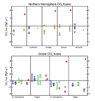
Figure 7.7. Regional ocean-atmosphere and land-atmosphere CO2 fluxes for the NH (top) and the globe (bottom) from inversion ensembles and bottom-up studies. Fluxes to the atmosphere are positive and uptake has a negative sign. Inversion results all correspond to the post-Pinatubo period 1992 to 1996 . Orange: Bottom-up terrestrial fluxes from Pacala et al. 2001 [JoC, MoS] ( and Kurz and Apps 1999 ) ) for North America, from Janssens et al. 2003 [JoC] ) for Europe and from Shvidenko and Nilsson 2003 [JoC] ) plus Fang et al. 2001 [JoC] ) for North Asia (Asian Russia and China). Cyan (filled circles): Bottom-up ocean flux estimates from ( Takahashi, et al. 2002 ) ). Blue: ocean fluxes from atmospheric inversions. Green: terrestrial fluxes from inversion models. Magenta: total inversion fluxes. Red: fossil fuel emissions. The mean flux of different inversion ensembles is reported. Inversion errors for regional fluxes are not reported here; their values usually range between 0.5 and 1 GtC yr–1. Error bar: range of atmospheric inversion fluxes from the TAR. Squares: Gurney et al. 2002 [JoC, MoS, SRC] ) inversions using annual mean CO2 observations and 16 transport models. Circles: Gurney et al. 2003 [JoC, SRC] ) inversions using monthly CO2 observations and 13 transport models. Triangles: Peylin et al. 2005 [JoC, SRC] ) inversions with three transport models, three regional breakdowns and three inversion settings. Inverted triangles: Rödenbeck et al. 2003a [JoC, SRC] ) inversions where the fluxes are solved on the model grid using monthly flask data.
7.3.2.3.2 The bottom-up view: land and ocean observations and models
The range of carbon flux and inventory data enables quantification of the distribution and variability of CO2 fluxes between the Earth’s surface and the atmosphere. This is called the ‘bottom-up’ approach. The fluxes can be determined by measuring carbon stock changes at repeated intervals, from which time-integrated fluxes can be deduced, or by direct observations of the fluxes. The stock change approach includes basin-scale in situ measurements of dissolved and particulate organic and inorganic carbon or tracers in the ocean (e.g., Sabine et al., 2004a [JoC, SRC] ), extensive forest biomass inventories (e.g., UN-ECE/FAO, 2000; Fang et al., 2001 [JoC] ;( Goodale et al., 2002; ) ( Nabuurs et al., 2003; ) Shvidenko and Nilsson, 2003 [JoC] ) and soil carbon inventories and models (e.g., Ogle et al., 2003 [MoS] ; Bellamy et al., 2005 [JoC] ; van Wesemael et al., 2005 [MoS] ; Falloon et al., 2006 [MoS] ). The direct flux measurement approach includes surveys of ocean CO2 partial pressure (pCO2)from ship-based measurements, drifters and time series (e.g., Lefèvre et al., 1999 [JoC, ARC] ;( Takahashi et al., 2002 ) ), and ecosystem flux measurements via eddy covariance flux networks (e.g., Valentini et al., 2000 [JoC] ; Baldocchi et al., 2001 [JoC] ).
The air-sea CO2 fluxes consist of a superposition of natural and anthropogenic CO2 fluxes, with the former being globally nearly balanced (except for a small net outgassing associated with the input of carbon by rivers). ( Takahashi et al. 2002 ) ) present both surface ocean pCO2 and estimated atmosphere-ocean CO2 fluxes (used as prior knowledge in many atmospheric inversions) normalised to 1995 using National Centers for Environmental Prediction (NCEP)/National Center for Atmospheric Research (NCAR) 41-year mean monthly winds. Large annual CO2 fluxes to the ocean occur in the Southern Ocean subpolar regions (40°S–60°S), in the North Atlantic poleward of 30°N and in the North Pacific poleward of 30°N (see Figure 7.8 ). Ocean inversions calculate natural and anthropogenic air-sea fluxes ( Gloor et al., 2003 [JoC, MoS] ; Mikaloff Fletcher et al., 2006 [NPR, JoC, MoS] ), by optimising ocean carbon model results against vertical profiles of DIC data. These studies indicate that the Southern Ocean is the largest sink of anthropogenic CO2,together with mid- to high-latitude regions in the North Atlantic. This is consistent with global ocean hydrographic surveys ( Sabine et al., 2004a [JoC, SRC] and Figure 5.10 ). However, only half of the anthropogenic CO2 absorbed by the Southern Ocean is stored there, due to strong northward transport ( Mikaloff Fletcher et al., 2006 [NPR, JoC, MoS] ). The tropical Pacific is a broad area of natural CO2 outgassing to the atmosphere, but this region is a sink of anthropogenic CO2.
Models are used to extrapolate flux observations into regional estimates, using remote-sensing properties and knowledge of the processes controlling the CO2 fluxes and their variability. Rayner et al. 2005 [NPR, JoC, SRC] ) use inverse process-based models, where observations are ‘assimilated’ to infer optimised fluxes. Since the TAR, the global air-sea flux synthesis has been updated ( (Takahashi et al., 2002 ) and Figure 7.8 ), and new syntheses have been made of continental-scale carbon budgets of the NH continents ( Pacala et al., 2001 [JoC, MoS] ;( Goodale et al., 2002; ) Janssens et al., 2003 [JoC] ; Shvidenko and Nilsson, 2003 [JoC] ; Ciais et al., 2005a [NPR, SRC] ), and of tropical forests ( Malhi and Grace, 2000 [SRC] ). These estimates are shown in Figure 7.7 and compared with inversion results.
Comparing bottom-up regional fluxes with inversion results is not straightforward because: (1) inversion fluxes may contain a certain amount of prior knowledge of bottom-up fluxes so that the two approaches are not fully independent; (2) the time period for which inversion models and bottom-up estimates are compared is often not consistent, in the presence of interannual variations in fluxes [4] (see Section 7.3.2.4 ); and (3) inversions of CO2 data produce estimates of CO2 fluxes, so the results will differ from budgets for carbon fluxes (due to the emission of reduced carbon compounds that get oxidized into CO2 in the atmosphere and are subject to transport and chemistry) and carbon storage changes (due to lateral carbon transport, e.g., by rivers) ( Sarmiento and Sundquist, 1992 [JoC] ). Some of these effects can be included by ‘off-line’ conversion of inversion results ( Enting and Mansbridge, 1991 [JoC] ; Suntharalingam et al., 2005 [JoC] ). Reduced carbon compounds such as volatile organic compounds (VOCs), carbon monoxide (CO) and CH4 emitted by ecosystems and human activities are transported and oxidized into CO2 in the atmosphere ( Folberth et al., 2005 [JoC, SRC] ). Trade of forest and crop products displaces carbon from ecosystems ( Imhoff et al., 2004 [JoC] ). Rivers displace dissolved and particulate inorganic and organic carbon from land to ocean (e.g., Aumont et al., 2001 [JoC] ). A summary of the main results of inversion and bottom-up estimates of regional CO2 fluxes is given below.
7.3.2.3.3 Robust findings of regional land-atmosphere flux
• Tropical lands are found in inversions to be either carbon neutral or sink regions, despite widespread deforestation, as is apparent in Figure 7.7 ,where emissions from land include deforestation. This implies carbon uptake by undisturbed tropical ecosystems, in agreement with limited forest inventory data in the Amazon ( Phillips et al., 1998 [JoC] ; Malhi and Grace, 2000 [SRC] ).
• Inversions place a substantial land carbon sink in the NH. The inversion estimate is –1.7 (–0.4 to –2.3) GtC yr–1 (from data in Figure 7.7 ). A bottom-up value of the NH land sink of –0.98 (–0.38 to –1.6) GtC yr–1 was also estimated, based upon regional synthesis studies ( (Kurz and Apps, 1999; ) Fang et al., 2001 [JoC] ; Pacala et al., 2001 [JoC, MoS] ; Janssens et al., 2003 [JoC] ;( Nilsson et al., 2003; ) Shvidenko and Nilsson, 2003 [JoC] ). The inversion sink value is on average higher than the bottom-up value. Part of this discrepancy could be explained by lateral transport of carbon via rivers, crop trade and emission of reduced carbon compounds.
• The longitudinal partitioning of the northern land sink between North America, Europe and Northern Asia has large uncertainties (see Figure 7.7 ). Inversions give a very large spread over Europe (–0.9 to +0.2 GtC yr–1), and Northern Asia (–1.2 to +0.3 GtC yr–1)and a large spread over North America (–0.6 to –1.1 GtC yr–1). Within the uncertainties of each approach, continental-scale carbon fluxes from bottom-up and top-down methods over Europe, North America and Northern Asia are mutually consistent ( Pacala et al., 2001 [JoC, MoS] ; Janssens et al., 2003 [JoC] ). The North American carbon sink estimated by recent inversions is on average lower than an earlier widely cited study by Fan et al. 1998 [JoC, MoS] ). Nevertheless, the Fan et al. 1998 [JoC, MoS] ) estimate remains within the range of inversion uncertainties. In addition, the fluxes calculated in Fan et al. 1998 [JoC, MoS] ) coincide with the low growth rate post-Pinatubo period, and hence are not necessarily representative of long-term behaviour.
7.3.2.3.4 Robust findings of regional ocean-atmosphere flux
• The regional air-sea CO2 fluxes consist of a superposition of natural and anthropogenic CO2 fluxes, with the former being globally nearly balanced (except for a small net outgassing associated with the input of carbon by rivers), and the latter having a global integral uptake of 2.2 ± 0.5 GtC yr–1 (see Table 7.1 ).
• The tropical oceans are outgassing CO2 to the atmosphere (see Figure 7.8 ), with a mean flux of the order of 0.7 GtC yr–1,estimated from an oceanic inversion ( Gloor et al., 2003 [JoC, MoS] ), in good agreement with atmospheric inversions (0 to 1.5 GtC yr–1), and estimates based on oceanic pCO2 observations (0.8 GtC yr–1( ;Takahashi et al., 2002 ) ).
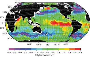
Figure 7.8. Estimates (4° × 5°) of sea-to-air flux of CO2,computed using 940,000 measurements of surface water pCO2 collected since 1956 and averaged monthly, together with NCEP/NCAR 41-year mean monthly wind speeds and a (10-m wind speed)2 dependence on the gas transfer rate Wanninkhof, dependence on the gas transfer rate Wanninkhof,). The fluxes were normalised to the year 1995 using techniques described in ( Takahashi et al. 2002 ) ), who used wind speeds taken at the 0.995 standard deviation level (about 40 m above the sea surface). The annual flux of CO2 for 1995 with 10-m winds is –1.6 GtC yr–1,with an approximate uncertainty (see Footnote 1) of ±1 GtC yr–1,mainly due to uncertainty in the gas exchange velocity and limited data coverage. This estimated global flux consists of an uptake of anthropogenic CO2 of –2.2 GtC yr–1 (see text) plus an outgassing of 0.6 GtC yr–1,corresponding primarily to oxidation of organic carbon borne by rivers (Figure 7.3). The monthly flux values with 10-m winds used here are available from T. Takahashi at http://www.ldeo.columbia.edu/res/pi/CO2/carbondioxide/pages/air_sea_flux_rev1.html.
• The extratropical NH ocean is a net sink for anthropogenic and natural CO2,with a magnitude of the order of 1.2 GtC yr–1,consistent among various estimates.
• The Southern Ocean is a large sink of atmospheric CO2( (Takahashi et al., 2002; ) Gurney et al., 2002 [JoC, MoS, SRC] ) and of anthropogenic CO2 ( Gloor et al., 2003 [JoC, MoS] ; Mikaloff Fletcher et al., 2006 [NPR, JoC, MoS] ). Its magnitude has been estimated to be about 1.5 GtC yr–1.This estimate is consistent among the different methods at the scale of the entire Southern Ocean. However, differences persist with regard to the Southern Ocean flux distribution between subpolar and polar latitudes (T. Roy et al., 2003 [Ambiguous] ). Atmospheric inversions and oceanic inversions indicate a larger sink in subpolar regions ( Gurney et al., 2002 [JoC, MoS, SRC] ; Gloor et al., 2003 [JoC, MoS] ), consistent with the distribution of CO2 fluxes based on available ∆pCO2 observations( Figure 7.8 ( and Takahashi, 2002 ) ).
7.3.2.4 Interannual Changes in the Carbon Cycle
7.3.2.4.1 Interannual changes in global fluxes
The atmospheric CO2 growth rate exhibits large interannual variations (see Figure 3.3 ,the TAR and http://lgmacweb.env.uea.ac.uk/lequere/co2/carbon_budget). The variability of fossil fuel emissions and the estimated variability in net ocean uptake are too small to account for this signal, which must be caused by year-to-year fluctuations in land-atmosphere fluxes. Over the past two decades, higher than decadal-mean CO2 growth rates occurred in 1983, 1987, 1994 to 1995, 1997 to 1998 and 2002 to 2003 . During such episodes, the net uptake of anthropogenic CO2 (sum of land and ocean sinks) is temporarily weakened. Conversely, small growth rates occurred in 1981, 1992 to 1993 and 1996 to 1997, associated with enhanced uptake. Generally, high CO2 growth rates correspond to El Niño climate conditions, and low growth rates to la Niña ( Bacastow and Keeling, 1981 [NPR, MoS, ARC] ; Lintner, 2002 [JoC] ). However, two episodes of CO2 growth rate variations during the past two decades did not reflect such an El Niño forcing. In 1992 to 1993, a marked reduction in growth rate occurred, coincident with the cooling and radiation anomaly caused by the eruption of Mt. Pinatubo in June 1991 . In 2002 to 2003, an increase in growth rate occurred, larger than expected based on the very weak El Niño event ( Jones and Cox, 2005 [JoC, SRC] ). It coincided with droughts in Europe ( Ciais et al., 2005b [JoC, SRC] ), in North America ( Breshears et al., 2005 [JoC] ) and in Asian Russia ( IFFN, 2003 [NPR] ).
Since the TAR, many studies have confirmed that the variability of CO2 fluxes is mostly due to land fluxes, and that tropical lands contribute strongly to this signal( Figure 7.9 ). A predominantly terrestrial origin of the growth rate variability can be inferred from (1) atmospheric inversions assimilating time series of CO2 concentrations from different stations ( Bousquet et al., 2000 [JoC, SRC] ; Rödenbeck et al., 2003b [SRC] ; Baker et al., 2006 [JoC, MoS, SRC] ), (2) consistent relationships between δ13C and CO2 ( Rayner et al., 1999 [JoC, SRC] ), (3) ocean model simulations (e.g., le Quéré et al., 2003 [JoC, SRC] ; McKinley et al., 2004a [JoC] ) and (4) terrestrial carbon cycle and coupled model simulations (e.g., C. Jones et al., 2001 [Ambiguous] ; McGuire et al., 2001 [JoC, MoS] ; Peylin et al., 2005 [JoC, SRC] ; Zeng et al., 2005 [JoC] ). Currently, there is no evidence for basin-scale interannual variability of the air-sea CO2 flux exceeding ±0.4 GtC yr–1,but there are large ocean regions, such as the Southern Ocean, where interannual variability has not been well observed.
7.3.2.4.2 Interannual variability in regional fluxes, atmospheric inversions and bottom-up models
Year-to-year flux anomalies can be more robustly inferred by atmospheric inversions than mean fluxes. Yet, at the scale of continents or ocean basins, the inversion errors increase and the statistical significance of the inferred regional fluxes decreases. [5] This is why Figure 7.9 shows the land-atmosphere and ocean-atmosphere flux anomalies over broad latitude bands only for the inversion ensembles of Baker et al. 2006 [JoC, MoS, SRC] Bousquet et al. 2000 [JoC, SRC] and Rödenbeck et al. 2003b [SRC] ). An important finding of these studies is that differences in transport models have little impact on the interannual variability of fluxes. Interannual variability of global land-atmosphere fluxes (±4 GtC yr–1 between extremes) is larger than that of air-sea fluxes and dominates the global fluxes. This result is also true over large latitude bands( Figure 7.9 ). Tropical land fluxes exhibit on average a larger variability than temperate and boreal fluxes. Inversions give tropical land flux anomalies of the order of ±1.5 to 2 GtC yr–1,which compare well in timing and magnitude with terrestrial model results ( Tian et al., 1998 [JoC] ; Peylin et al., 2005 [JoC, SRC] ; Zeng et al., 2005 [JoC] ). In these studies, enhanced sources occur during El Niño episodes and abnormal sinks during la Niña. In addition to the influence of these climate variations on ecosystem processes ( Gérard et al., 1999 [JoC] ; C. Jones et al., 2001 [Ambiguous] ), regional droughts during El Niño events promote large biomass fires, which appear to contribute to high CO2 growth rates during the El Niño episodes ( Barbosa et al., 1999 [JoC] ; Langenfelds et al., 2002 [JoC] ; Page et al., 2002 [JoC] ;( van der Werf et al., 2003, ) 2004; Patra et al., 2005 [JoC, MoS] ).
Inversions robustly attribute little variability to ocean-atmosphere CO2 flux (±0.5 GtC yr–1 between extremes), except for the recent work of Patra et al. 2005 [JoC, MoS] ). This is in agreement with ocean model and ocean observations ( Lee et al., 1998 [JoC] ; le Quéré et al., 2003 [JoC, SRC] ; Obata and Kitamura, 2003 [JoC, MoS] ; McKinley et al., 2004b [JoC, MoS] ). However, inversions and ocean models differ on the dominant geographic contributions to the variability. Inversions estimate similar variability in both hemispheres, whereas ocean models estimate more variability in the Southern Ocean ( Bousquet et al., 2000 [JoC, SRC] ; Rödenbeck et al., 2003b [SRC] ; Baker et al., 2006 [JoC, MoS, SRC] ). Over the North Atlantic, Gruber et al. 2002 [JoC, SRC] ) suggest a regional CO2 flux variability (extremes of ±0.3 GtC yr–1)by extrapolating data from a single ocean station, but McKinley et al. 2004a [JoC] ,b) model a small variability (extremes of ±0.1 GtC yr–1). The equatorial Pacific is the ocean region of the world where the variability is constrained with repeated ∆pCO2 observations (variations of about ±0.4 GtC yr–1 ;Feely et al., 2002 [ARC] ), with a reduced source of CO2 during El Niño associated with decreased upwelling of CO2-rich waters. Over this region, some inversion results (e.g., Bousquet et al., 2000 [JoC, SRC] ) compare well in magnitude and timing with ocean and coupled model results ( Le Quéré et al., 2000 [JoC, SRC] ; C. Jones et al., 2001 [Ambiguous] ; McKinley et al., 2004a [JoC] ,b) and with ∆pCO2 observations ( Feely et al., 1999 [JoC, ARC] , 2002 ).
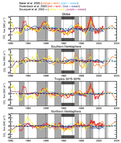
Figure 7.9. Year-to-year anomalies in ocean-atmosphere and land-atmosphere CO2 fluxes (GtC yr–1)from interannual inversion ensembles covering the past 20 years or so, grouped into large latitude bands, and over the globe. Three different inversion ensembles from Bousquet et al. 2000 [JoC, SRC] Rödenbeck et al. 2003a [JoC, SRC] and Baker et al. 2006 [JoC, MoS, SRC] ) are shown. For each flux and each region, the anomalies were obtained by subtracting the long-term mean flux and removing the seasonal signal. Grey shaded regions indicate El Niño episodes, and the black bars indicate the cooling period following the Mt. Pinatubo eruption.
7.3.2.4.3 Slowdown in carbon dioxide growth rates during the early 1990s
The early 1990 s had anomalously strong global sinks for atmospheric CO2,compared with the decadal mean( Table 7.1 ). Although a weak El Niño from 1991 to 1995 may have helped to enhance ocean uptake at that time, inversions andO2:N2 and δ13C-CO2 atmospheric data ( Battle et al., 2000 [JoC] ) indicate that the enhanced uptake was of predominantly terrestrial origin. The regions where the 1992 to 1993 abnormal sink is projected to be are not robustly estimated by inversions. Both Bousquet et al. 2000 [JoC, SRC] and Rödenbeck et al. 2003b [SRC] ) project a large fraction of that sink in temperate North America, while Baker et al. 2006 [JoC, MoS, SRC] ) place it predominantly in the tropics. Model results suggest that cooler temperatures caused by the Mt. Pinatubo eruption reduced soil respiration and enhanced NH carbon uptake ( Jones and Cox, 2001b [NPR, SRC] ; Lucht et al., 2002 [JoC] ), despite lower productivity as indicated by remote sensing of vegetation activity. In addition, aerosols from the volcanic eruption scattered sunlight and increased its diffuse fraction, which is used more efficiently by plant canopies in photosynthesis than direct light ( Gu et al., 2003 [JoC] ). It has been hypothesised that a transient increase in the diffuse fraction of radiation enhanced CO2 uptake by land ecosystems in 1992 to 1993, but the global significance and magnitude of this effect remains unresolved ( (Roderick et al., 2001; ) Krakauer and Randerson, 2003 [JoC] ; Angert et al., 2004 [JoC] ; Robock, 2005 [JoC] ).
7.3.2.4.4 Speed-up in carbon dioxide growth rates during the late 1990s
The high CO2 growth in 1998 coincided with a global increase in CO concentrations attributable to wildfires ( (Yurganov et al., 2005 ) ) in Southeast Asia (60%), South America (30%) and Siberia ( van der Werf et al., 2004 [JoC] Langenfelds et al. 2002 [JoC] ) analyse the correlations in the interannual growth rate of CO2 and other species at 10 stations and link the 1997 to 1998 (and the 1994 to 1995 ) anomalies to high fire emissions as a single process. Achard et al. 2004 [JoC, MoS] ) estimate a source of 0.88 ± 0.07 GtC emitted from the burning of 2.4 × 10⁶ ha of peatland in the Indonesian forest fires in 1997 to 1998, and Page et al. 2002 [JoC] ) estimate a source of +0.8 to +2.6 GtC. During the 1997 to 1998 high CO2 growth rate episode, inversions place an abnormal source over tropical Southeast Asia, in good agreement with such bottom-up evidence. The relationship between El Niño and CO2 emissions from fires is not uniform: fire emissions from low productivity ecosystems in Africa and northern Australia are limited by fuel load density and thus decrease during drier periods, in contrast to the response in tropical forests ( Barbosa et al., 1999 [JoC] ; Randerson et al., 2005 [JoC] ). In addition, co-varying processes such as reduced productivity caused by drought in tropical forests during El Niño episodes may be superimposed on fire emissions. From 1998 to 2003, extensive drought in mid-latitudes of the NH ( Hoerling and Kumar, 2003 [JoC] ), accompanied by more wildfires in some regions ( Balzter et al., 2005 [JoC] ;( Yurganov et al., 2005 ) ) may have led to decreased photosynthesis and carbon uptake ( Angert et al., 2005 [JoC] ; Ciais et al., 2005b [JoC, SRC] ), helping to increase the atmospheric CO2 growth rate.
7.3.3 Terrestrial Carbon Cycle Processes and Feedbacks to Climate
The net exchange of carbon between the terrestrial biosphere and the atmosphere is the difference between carbon uptake by photosynthesis and release by plant respiration, soil respiration and disturbance processes (fire, windthrow, insect attack and herbivory in unmanaged systems, together with deforestation, afforestation, land management and harvest in managed systems). Over at least the last 30 years, the net result of all these processes has been uptake of atmospheric CO2 by terrestrial ecosystems( Table 7.1 ,‘land-atmosphere flux’ row). It is critical to understand the reasons for this uptake and its likely future course. Will uptake by the terrestrial biosphere grow or diminish with time, or even reverse so that the terrestrial biosphere becomes a net source of CO2 to the atmosphere? To answer this question it is necessary to understand the underlying processes and their dependence on the key drivers of climate, atmospheric composition and human land management.
Drivers that affect the carbon cycle in terrestrial ecosystems can be classified as (1) direct climate effects (changes in precipitation, temperature and radiation regime); (2) atmospheric composition effects (CO2 fertilization, nutrient deposition, damage by pollution); and (3) land use change effects (deforestation, afforestation, agricultural practices, and their legacies over time). This section first summarises current knowledge of the processes by which each of these drivers influence the terrestrial carbon balance, and then examines knowledge of the integrative consequences of all these processes in the key case of tropical forests.
7.3.3.1 Processes Driven by Climate, Atmospheric Composition and Land Use Change
7.3.3.1.1 Climatic regulation of terrestrial carbon exchange
Ecosystem responses to environmental drivers (sunlight, temperature, soil moisture) and to ecological factors (e.g., forest age, nutrient supply, organic substrate availability; see, e.g., Clark, 2002 [SRC] ; Ciais et al., 2005b [JoC, SRC] ; Dunn et al., 2007 [2007] ) are complex. For example, elevated temperature and higher soil water content enhance rates for heterotrophic respiration in well-aerated soils, but depress these rates in wet soils. Soil warming experiments typically show marked soil respiration increases at elevated temperature ( Oechel et al., 2000 [JoC] ;( Rustad et al., 2001; ) Melillo et al., 2002 [JoC] ), but CO2 fluxes return to initial levels in a few years as pools of organic substrate re-equilibrate with inputs ( Knorr et al., 2005 [JoC, SRC] ). However, in dry soils, decomposition may be limited by moisture and not respond to temperature ( Luo et al., 2001 [JoC, ARC] ). Carbon cycle simulations need to capture both the short- and long-term responses to changing climate to predict carbon cycle responses.
Current models of terrestrial carbon balance have difficulty simulating measured carbon fluxes over the full range of temporal and spatial scales, including instantaneous carbon exchanges at the leaf, plot or ecosystem level, seasonal and annual carbon fluxes at the stand level and decadal to centennial accumulation of biomass and organic matter at stand or regional scales ( Melillo et al., 1995 [JoC, MoS] ; Thornton et al., 2002 [MoS] ). Moreover, projections of changes in land carbon storage are tied not only to ecosystem responses to climate change, but also to the modelled projections of climate change itself. As there are strong feedbacks between these components of the Earth system (see Section 7.3.5 ), future projections must be considered cautiously.
7.3.3.1.2 Effects of elevated carbon dioxide
On physiological grounds, almost all models predict stimulation of carbon assimilation and sequestration in response to rising CO2,called ‘CO2 fertilization’ ( Cramer et al., 2001 [MoS] ; Oren et al., 2001 [JoC] ; Luo et al., 2004 [ARC] ; DeLucia et al., 2005 ). Free Air CO2 Enrichment (FACE) and chamber studies have been used to examine the response of ecosystems to large (usually about 50%) step increases in CO2 concentration. The results have been variable (e.g., Oren et al., 2001 [JoC] ; Nowak et al., 2004 [MoS] ; Norby et al., 2005 [JoC] ). On average, net CO2 uptake has been stimulated, but not as much as predicted by some models. Other factors (e.g., nutrients or genetic limitations on growth) can limit plant growth and reduce response to CO2.Eleven FACE experiments, encompassing bogs, grasslands, desert and young temperate tree stands report an average increased net primary productivity (NPP) of 12% when compared to ambient CO2 levels ( Nowak et al., 2004 [MoS] ). There is a large range of responses, with woody plants consistently showing NPP increases of 23 to 25% ( Norby et al., 2005 [JoC] ), but much smaller increases for grain crops ( (Ainsworth and Long, 2005 ) ), reflecting differential allocation of the incremental organic matter to shorter- vs. longer-lived compartments. Overall, about two-thirds of the experiments show positive response to increased CO2( (Ainsworth and Long, 2005; ) Luo et al., 2005 [JoC] ). Since saturation of CO2 stimulation due to nutrient or other limitations is common ( (Dukes et al., 2005; ) Koerner et al., 2005 [JoC] ), it is not yet clear how strong the CO2 fertilization effect actually is.
7.3.3.1.3 Nutrient and ozone limitations to carbon sequestration
The basic biochemistry of photosynthesis implies that stimulation of growth will saturate under high CO2 concentrations and be further limited by nutrient availability ( (Dukes et al., 2005; ) Koerner et al., 2005 [JoC] ) and by possible acclimation of plants to high CO2 levels ( (Ainsworth and Long, 2005 ) ). Carbon storage by terrestrial plants requires net assimilation of nutrients, especially N, a primary limiting nutrient at middle and high latitudes and an important nutrient at lower latitudes ( Vitousek et al., 1998 [NPR] Hungate et al. 2003 [JoC] ) argue that ‘soil C sequestration under elevated CO2 is constrained both directly by N availability and indirectly by nutrients needed to supportN2 fixation’, and Reich et al. 2006 [JoC] ) conclude that ‘soil N supply is probably an important constraint on global terrestrial responses to elevated CO2’. This view appears to be consistent with other recent studies (e.g., Finzie et al., 2006; ( Norby et al., 2006; ) van Groenigen et al., 2006 [JoC] ) and with at least some of the FACE data, further complicating estimation of the current effects of rising CO2 on carbon sequestration globally.
Additional N supplied through atmospheric deposition or direct fertilization can stimulate plant growth ( Vitousek, 2004 [NPR, MoS] ) and in principle could relieve the nutrient constraint on CO2 fertilization. Direct canopy uptake of atmospheric N may be particularly effective ( Sievering et al., 2000 [JoC] ). Overall, the effectiveness of N inputs appears to be limited by immobilisation and other mechanisms. For example, when labelled nitrogen(15N) was added to soil and litter in a forest over seven years, only a small fraction became available for tree growth ( (Nadelhoffer et al., 2004 ) ). Moreover, atmospheric N deposition is spatially correlated with air pollution, including elevated atmospheric ozone. Ozone and other pollutants may have detrimental effects on plant growth, possibly further limiting the stimulation of carbon uptake by anthropogenic N emissions ( (Ollinger and Aber, 2002; ) Holland and Carroll, 2003 [NPR, SRC] ). Indeed, Felzer et al. 2004 [JoC, MoS] ) estimate that surface ozone increases since 1950 may have reduced CO2 sequestration in the USA by 18 to 20 TgC yr–1.The current generation of coupled carbon-climate models (see Section 7.3.5 )does not include nutrient limitations or air pollution effects.
7.3.3.1.4 Fire
Fire is a major agent for conversion of biomass and soil organic matter to CO2( (Randerson et al., 2002a ) –d; Cochrane, 2003 [JoC] ;( Nepstad et al., 2004; ) Jones and Cox, 2005 [JoC, SRC] ; Kasischke et al., 2005 [JoC] ; Randerson et al., 2005 [JoC] ). Globally, wildfires (savannah and forest fires, excluding biomass burning for fuel and land clearing) oxidize 1.7 to 4.1 GtC yr–1 ( Mack et al., 1996 [NPR, MoS] ; Andreae and Merlet, 2001 [JoC] ), or about 3 to 8% of total terrestrial NPP. There is an additional large enhancement of CO2 emissions associated with fires stimulated by human activities, such as deforestation and tropical agricultural development. Thus, there is a large potential for future alteration in the terrestrial carbon balance through altered fire regimes. A striking example occurred during the 1997 to 1998 El Niño, when large fires in the Southeast Asian archipelago are estimated to have released 0.8 to 2.6 GtC (see Section 7.3.2.4 ). Fire frequency and intensity are strongly sensitive to climate change and variability, and to land use practices. Over the last century, trends in burned area have been largely driven by land use practices, through fire suppression policies in mid-latitude temperate regions and increased use of fire to clear forest in tropical regions ( (Mouillot and Field, 2005 ) ). However, there is also evidence that climate change has contributed to an increase in fire frequency in Canada ( Gillett et al., 2004 [JoC, ARC] ). The decrease in fire frequency in regions like the USA and Europe has contributed to the land carbon sink there, while increased fire frequency in regions like Amazonia, Southeast Asia and Canada has contributed to the carbon source. At high latitudes, the role of fire appears to have increased in recent decades: fire disturbance in boreal forests was higher in the 1980 s than in any previous decade on record ( Kurz et al., 1995 [JoC] ;( Kurz and Apps, 1999; ) Moulliot ( and Field, 2005 ) Flannigan et al. 2005 [NotFound] ) estimate that in the future, the CO2 source from fire will increase.
7.3.3.1.5 Direct effects of land use and land management
Evolution of landscape structure, including woody thickening: Changes in the structure and distribution of ecosystems are driven in part by changes in climate and atmospheric CO2,but also by human alterations of landscapes through land management and the introduction of invasive species and exotic pathogens. The single most important process in the latter category is woody encroachment or vegetation thickening, the increase in woody biomass occurring in (mainly semi-arid) grazing lands. In many regions, this increase arises from fire suppression and associated grazing management practices, but there is also a possibility that increases in CO2 are givingC3 woody plants a competitive advantage overC4 grasses ( (Bond et al., 2003 ) ). Woody encroachment could account for as much as 22 to 40% of the regional carbon sink in the USA ( Pacala et al., 2001 [JoC, MoS] ), and a high proportion in northeast Australia ( (Burrows et al., 2002 ) ). Comprehensive data are lacking to define this effect accurately.
Deforestation: Forest clearing (mainly in the tropics) is a large contributor to the land use change component of the current atmospheric CO2 budget, accounting for up to one-third of total anthropogenic emissions (see Table 7.2 ; Section 7.3.2.1 ;also Table 7.1 ,row ‘land use change flux’). The future evolution of this term in the CO2 budget is therefore of critical importance. Deforestation in Africa, Asia and the tropical Americas is expected to decrease towards the end of the 21st century to a small fraction of the levels in 1990 ( IPCC, 2000 [NPR] ). The declines in Asia and Africa are driven by the depletion of forests, while trends in the Americas have the highest uncertainty given the extent of the forest resource.
Afforestation: Recent (since 1970 ) afforestation and reforestation as direct human-induced activities have not yet had much impact on the global terrestrial carbon sink. However, regional sinks have been created in areas such as China, where afforestation since the 1970 s has sequestered 0.45 GtC ( Fang et al., 2001 [JoC] ). The largest effect of afforestation is not immediate but through its legacy.
Agricultural practices: Improvement of agricultural practices on carbon-depleted soils has created a carbon sink. For instance, the introduction of conservation tillage in the USA is estimated to have increased soil organic matter (SOM) stocks by about 1.4 GtC over the last 30 years. However, yearly increases in SOM can be sustained only for 50 to 100 years, after which the system reaches a new equilibrium ( Cole et al., 1996 [NPR] ; Smith et al., 1997 [MoS] ). Moreover, modern conservation tillage often entails large inputs of chemicals and fertilizer, which are made using fossil fuels, reducing the CO2 benefit from carbon sequestration in agricultural soils. The increase in soil carbon stocks under low-tillage systems may also be mostly a topsoil effect with little increase in total profile carbon storage observed, confounded by the fact that most studies of low-tillage systems have only sampled the uppermost soil layers.
7.3.3.1.6 Forest regrowth
Some studies suggest that forest regrowth could be a major contributor to the global land carbon sink (e.g., Pacala et al., 2001 [JoC, MoS] ; Schimel et al., 2001 [JoC] ; Hurtt et al., 2002 [JoC, MoS] ). Forest areas generally increased during the 20th century at middle and high latitudes (unlike in the tropics). This surprising trend reflects the intensification of agriculture and forestry. Globally, more food is being grown on less land, reflecting mechanisation of agriculture, increased fertilizer use and adoption of high-yield cultivars, although in parts of Africa and Asia the opposite is occurring. Likewise, intensive forest management and agroforestry produce more fibre on less land; improved forest management favours more rapid regrowth of forests after harvest. These trends have led to carbon sequestration by regrowing forests. It should be noted, however, that industrialised agriculture and forestry require high inputs of fossil energy, so it is difficult to assess the net global effects of agricultural intensification on atmospheric greenhouse gases and radiative forcing.
Regional studies have confirmed the plausibility of strong mid-latitude sinks due to forest regrowth. Data from the eddy flux tower network show that forests on long-abandoned former agricultural lands ( Curtis et al., 2002 [MoS] ) and in industrial managed forests (Hollinger et al., 2002 [NotFound] ) take up significant amounts of carbon every year. Analysis of forest inventory data shows that, in aggregate, current forest lands are significant sinks for atmospheric CO2 ( Pacala et al., 2001 [JoC, MoS] ). Few old growth forests remain at mid-latitudes (most forests are less than 70 years old), in part due to forest management. Therefore, forests in these areas are accumulating biomass because of their ages and stages of succession. Within wide error bands (see Section 7.3.2.3 ), the uptake rates inferred from flux towers are generally consistent with those inferred from inverse methods (e.g., Hurtt et al., 2002 [JoC, MoS] ). Stocks of soil carbon are also likely increasing due to replenishment of soil organic matter and necromass depleted during the agricultural phase, and changes in soil microclimate associated with reforestation; these effects might add 30 to 50% to the quantity of CO2 sequestered (e.g., Barford et al., 2001 [JoC] ). It is important to note that at least some of this sequestration is ‘refilling’ the deficits in biomass and soil organic matter, accumulated in previous epochs (see Figure 7.3 ), and the associated CO2 uptake should be expected to decline in the coming decades unless sustained by careful management strategies designed to accomplish that purpose.
7.3.4 Ocean Carbon Cycle Processes and Feedbacks to Climate
7.3.4.1 Overview of the Ocean Carbon Cycle
Oceanic carbon exists in several forms: as DIC, DOC, and particulate organic carbon (POC) (living and dead) in an approximate ratio DIC:DOC:POC = 2000 :38:1 (about 37,000 GtC DIC: Falkowski et al., 2000 [JoC] and Sarmiento and Gruber, 2006 [NPR, SRC] ; 685 GtC DOC: Hansell and Carlson, 1998 [JoC] ; and 13 to 23 GtC POC: Eglinton and Repeta, 2004 [NPR] ). Before the industrial revolution, the ocean contained about 60 times as much carbon as the atmosphere and 20 times as much carbon as the terrestrial biosphere/soil compartment.
Seawater can, through inorganic processes, absorb large amounts of CO2 from the atmosphere, because CO2 is a weakly acidic gas and the minerals dissolved in the ocean have over geologic time created a slightly alkaline ocean (surface pH 7.9 to 8.25: Degens et al., 1984 [NPR] ; Royal Society, 2005 [NPR] ). The air-sea exchange of CO2 is determined largely by the air-sea gradient in pCO2 between atmosphere and ocean. Equilibration of surface ocean and atmosphere occurs on a time scale of roughly one year. Gas exchange rates increase with wind speed ( Wanninkhof and McGillis, 1999 [JoC, ARC] ; Nightingale et al., 2000 [JoC] ) and depend on other factors such as precipitation, heat flux, sea ice and surfactants. The magnitudes and uncertainties in local gas exchange rates are maximal at high wind speeds. In contrast, the equilibrium values for partitioning of CO2 between air and seawater and associated seawater pH values are well established ( Zeebe and Wolf-Gladrow, 2001 [NPR] ; see Box 7.3 ).
Box 7.3: Marine Carbon Chemistry and Ocean Acidification
The marine carbonate buffer system allows the ocean to take up CO2 far in excess of its potential uptake capacity based on solubility alone, and in doing so controls the pH of the ocean. This control is achieved by a series of reactions that transform carbon added as CO2 into HCO3– and CO32–.These three dissolved forms (collectively known as DIC) are found in the approximate ratio CO2:HCO3–:CO32– of 1:100:10 (Equation (7.1)). CO2 is a weak acid and when it dissolves, it reacts with water to form carbonic acid, which dissociates into a hydrogen ion (H+)and a HCO3– ion, with some of theH+ then reacting with CO32– to form a second HCO3– ion (Equation (7.2)).
| CO2 +H2O→H+ + HCO3– → 2H+ + CO32– | (7.1) |
| CO2 +H2O+ CO32– → HCO3– +H+ + CO32– → 2HCO3– | (7.2) |
Therefore, the net result of adding CO2 to seawater is an increase inH+ and HCO3–,but a reduction in CO32–.The decrease in the CO32– ion reduces the overall buffering capacity as CO2 increases, with the result that proportionally moreH+ ions remain in solution and increase acidity.
This ocean acidification is leading to a decrease in the saturation state of CaCO3 in the ocean. Two primary effects are expected: (1) the biological production of corals as well as calcifying phytoplankton and zooplankton within the water column may be inhibited or slowed down (Royal Society, 2005 [NPR] ), and (2) the dissolution of CaCO3 at the ocean floor will be enhanced ( Archer, 2005 [JoC, SRC] ). Aragonite, the meta-stable form of CaCO3 produced by corals and pteropods (planktonic snails; Lalli and Gilmer, 1989 [NPR] ), will be particularly susceptible to a pH reduction ( Kleypas et al., 1999b [JoC] ; Hughes et al., 2003 [JoC] ; Orr et al., 2005 [JoC, ARC] ). Laboratory experiments under high ambient CO2 with the coccolithophore species Emiliania huxleyi and Gephyrocapsa oceanica produce a significant reduction in CaCO3 production and a stimulation of POC production ( Riebesell et al., 2000 [JoC, SRC] ; Zondervan et al., 2001 [JoC, SRC] ). Other species and growth under other conditions may show different responses, so that no conclusive quantification of the CaCO3 feedback is possible at present ( (Tortell et al., 2002; ) ( Sciandra et al., 2003 ) ).
The sinking speed of marine particle aggregates depends on their composition: CaCO3 may act as an efficient ballast component, leading to high sinking speeds of aggregates ( Armstrong et al., 2002 [MoS] ; Klaas and Archer, 2002 [JoC] ). The relatively small negative feedback of reduced CaCO3 production to atmospheric pCO2 may be compensated for by a change in the ballast for settling biogenic particles and the associated shallowing of re-mineralization depth levels in the water column for organic carbon ( Heinze, 2004 [JoC, MoS, SRC] ). On the other hand, production of extracellular organic carbon could increase under high CO2 levels and lead to an increase in export ( Engel et al., 2004 [JoC] ).
Ecological changes due to expected ocean acidification may be severe for corals in tropical and cold waters ( (Gattuso et al., 1999; ) ( Kleypas et al., 1999a; ) Langdon et al., 2003 [JoC] ; Buddemeier et al., 2004 [NPR] ; Roberts et al., 2006 [JoC] ) and for pelagic ecosystems ( (Tortell et al., 2002; ) Royal Society, 2005 [NPR] ). Acidification can influence the marine food web at higher trophic levels ( (Langenbuch and Pörtner, 2003; ) ( Ishimatsu et al., 2004 ) ).
Since the beginning of the industrial revolution, sea surface pH has dropped by about 0.1 pH units (corresponding to a 30% increase in the H ion concentration). The expected continued decrease may lead within a few centuries to an ocean pH estimated to have occurred most recently a few hundred million years before present ( Caldeira and Wickett, 2003 [JoC] ; Key et al., 2004 [JoC] ; Box 7.3 ,Figure 1).
According to a model experiment based on the IPCC Scenarios 1992a (IS92a) emission scenario, bio-calcification will be reduced by 2100, in particular within the Southern Ocean ( Orr et al., 2005 [JoC, ARC] ), and by 2050 for aragonite-producing organisms (see also Figure 10.24 ). It is important to note that ocean acidification is not a direct consequence of climate change but a consequence of fossil fuel CO2 emissions, which are the main driver of the anticipated climate change
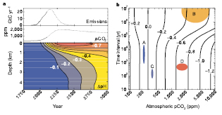
Box 7.3, Figure 1. (a) Atmospheric CO2 emissions, historical atmospheric CO2 levels and predicted CO2 concentrations from the given emission time series, together with changes in ocean pH based on horizontally averaged chemistry. The emission time series is based on the mid-range IS92a emission scenario (solid line) prior to 2100 and then assumes that emissions continue until fossil fuel reserves decline. (b) Estimated maximum change in surface ocean pH as a function of final atmospheric CO2 pressure, and the transition time over which this CO2 pressure is linearly approached from 280 ppm. A: Glacial-interglacial CO2 changes; B: slow changes over the past 300 Myr; C: historical changes in ocean surface waters; D: unabated fossil fuel burning over the next few centuries. Source: Caldeira and Wickett 2003 [JoC] ). Reprinted with permission from Macmillan Publishers Ltd: Nature, Caldeira and Wickett 2003 [JoC] ), copyright ( 2003 ).
In addition to changes in advection and mixing, the ocean can alter atmospheric CO2 concentration through three mechanisms ( Volk and Hoffert, 1985 [NPR] ), illustrated in Figure 7.10 :(1) absorption or release of CO2 due to changes in solubility of gaseous CO2 (‘solubility pump’); (2) changes in carbon fixation to POC in surface waters by photosynthesis and export of this carbon through sinking of organic particles out of the surface layer (‘organic carbon pump’) – this process is limited to first order by availability of light and nutrients (phosphate, nitrate, silicic acid and micronutrients such as iron); and (3) changes in the release of CO2 in surface waters during formation of CaCO3 shell material by plankton (‘CaCO3 counter pump’).
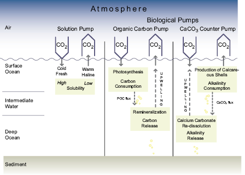
Figure 7.10. Three main ocean carbon pumps govern the regulation of natural atmospheric CO2 changes by the ocean ( Heinze et al., 1991 [JoC, MoS, SRC] ): the solubility pump, the organic carbon pump and the CaCO3 ‘counter pump’. The oceanic uptake of anthropogenic CO2 is dominated by inorganic carbon uptake at the ocean surface and physical transport of anthropogenic carbon from the surface to deeper layers. For a constant ocean circulation, to first order, the biological carbon pumps remain unaffected because nutrient cycling does not change. If the ocean circulation slows down, anthropogenic carbon uptake is dominated by inorganic buffering and physical transport as before, but the marine particle flux can reach greater depths if its sinking speed does not change, leading to a biologically induced negative feedback that is expected to be smaller than the positive feedback associated with a slower physical downward mixing of anthropogenic carbon. Reprinted with permission, copyright 1991 American Geophysical Union.
Organic particles are re-mineralized (oxidized to DIC and other inorganic compounds through the action of bacteria) primarily in the upper 1,000 m of the oceanic water column, with an accompanying decrease in dissolved O. On the average, CaCO3 particles sink deeper before they undergo dissolution: deep waters are undersaturated with respect to CaCO3.The remainder of the particle flux enters marine sediments and is subject to either re-dissolution within the water column or accumulation within the sediments. Although the POC reservoir is small, it plays an important role in keeping DIC concentrations low in surface waters and high in deep waters. The loop is closed through the three-dimensional ocean circulation: upwelling water brings inorganic carbon and nutrients to the surface again, leading to outgassing and biogenic particle production. Dissolved organic carbon enters the ocean water column from rivers and marine metabolic processes. A large fraction of DOC has a long ocean residence time (1–10 kyr), while other fractions are more short-lived (days to hundreds of years; Loh et al., 2004 [JoC] ). The composition of dissolved organic matter is still largely unknown.
In conjunction with the global ocean mixing or overturning time of the order of 1 kyr ( Broecker and Peng, 1982 [NPR, ARC] ), small changes in the large ocean carbon reservoir can induce significant changes in atmospheric CO2 concentration. Likewise, perturbations in the atmospheric pCO2 can be buffered by the ocean. Glacial-interglacial changes in the atmospheric CO2 content can potentially be attributed to a change in functioning of the marine carbon pump (see Chapter6 ). The key role for the timing of the anthropogenic carbon uptake by the ocean is played by the downward transport of surface water, with a high burden of anthropogenic carbon, into the ocean’s interior. The organic carbon cycle and the CaCO3 counter pump modulate, but do not dominate, the net marine uptake of anthropogenic carbon.
7.3.4.2 Carbon Cycle Feedbacks to Changes in Atmospheric Carbon Dioxide
Chemical buffering of anthropogenic CO2 is the quantitatively most important oceanic process acting as a carbon sink. Carbon dioxide entering the ocean is buffered due to scavenging by the CO32– ions and conversion to HCO3–,that is, the resulting increase in gaseous seawater CO2 concentration is smaller than the amount of CO2 added per unit of seawater volume. Carbon dioxide buffering in seawater is quantified by the Revelle factor (‘buffer factor’, Equation (7.3)), relating the fractional change in seawater pCO2 to the fractional change in total DIC after re-equilibration ( Revelle and Suess, 1957 [JoC] ; Zeebe and Wolf-Gladrow, 2001 [NPR] ):
Revelle factor (or buffer factor) = (Δ[CO2]/ [CO2]) / (Δ[DIC] / [DIC]) (7.3)
The lower the Revelle factor, the larger the buffer capacity of seawater. Variability of the buffer factor in the ocean depends mainly on changes in pCO2 and the ratio of DIC to total alkalinity. In the present-day ocean, the buffer factor varies between 8 and 13 ( Sabine et al., 2004a [JoC, SRC] ; Figure 7.11 ). With respect to atmospheric pCO2 alone, the inorganic carbon system of the ocean reacts in two ways: (1) seawater re-equilibrates, buffering a significant amount of CO2 from the atmosphere depending on the water volume exposed to equilibration; and (2) the Revelle factor increases with pCO2 (positive feedback; Figure 7.11 ). Both processes are quantitatively important. While the first is generally considered as a system response, the latter is a feedback process.
The ocean will become less alkaline (seawater pH will decrease) due to CO2 uptake from the atmosphere (see Box 7.3 ). The ocean’s capacity to buffer increasing atmospheric CO2 will decline in the future as ocean surface pCO2 increases( Figure 7.11 a). This anticipated change is certain, with potentially severe consequences.
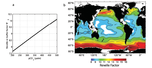
Figure 7.11. (a) The Revelle factor (or buffer factor) as a function of CO2 partial pressure (for temperature 25°C, salinity 35 psu, and total alkalinity 2,300 µmol kg–1 )(Zeebe and Wolf-Gladrow, 2001 [NPR] , page 73; reprinted with permission, copyright 2001 Elsevier). (b) The geographical distribution of the buffer factor in ocean surface waters in 1994 ( Sabine et al., 2004a [JoC, SRC] ; reprinted with permission, copyright 2004 American Association for the Advancement of Science). High values indicate a low buffer capacity of the surface waters.
Increased carbon storage in the deep ocean leads to the dissolution of calcareous sediments below their saturation depth ( Broecker and Takahashi, 1978 [NPR] ; Feely et al., 2004 [JoC, ARC] ). The feedback of CaCO3 sediment dissolution to atmospheric pCO2 increase is negative and quantitatively significant on a 1 to 100 kyr time scale, where CaCO3 dissolution will account for a 60 to 70% absorption of the anthropogenic CO2 emissions, while the ocean water column will account for 22 to 33% on a time scale of 0.1 to 1 kyr. In addition, the remaining 7 to 8% may be compensated by long-term terrestrial weathering cycles involving silicate carbonates ( Archer et al., 1998 [JoC, SRC] ). Due to the slow CaCO3 buffering mechanism (and the slow silicate weathering), atmospheric pCO2 will approach a new equilibrium asymptotically only after several tens of thousands of years ( Archer, 2005 [JoC, SRC] ; Figure 7.12 ).
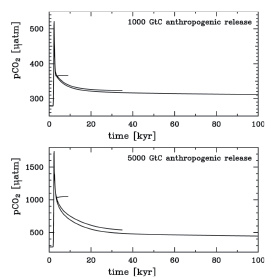
Figure 7.12. Model projections of the neutralization of anthropogenic CO2 for an ocean-only model, a model including dissolution of CaCO3 sediment and a model including weathering of silicate rocks, (top) for a total of 1,000 GtC of anthropogenic CO2 emissions and (bottom) for a total of 5,000 GtC of anthropogenic CO2.Note that the y-axis is different for the two diagrams. Without CaCO3 dissolution from the seafloor, the buffering of anthropogenic CO2 is limited. Even after 100 kyr, the remaining pCO2 is substantially higher than the pre-industrial value. Source: Archer 2005 [JoC, SRC] ).
Elevated ambient CO2 levels appear to also influence the production rate of POC by marine calcifying planktonic organisms (e.g., Zondervan et al., 2001 [JoC, SRC] ). This increased carbon fixation under higher CO2 levels was also observed for three diatom (siliceous phytoplankton) species ( Riebesell et al., 1993 [JoC, SRC] ). It is critical to know whether these increased carbon fixation rates translate into increased export production rates (i.e., removal of carbon to greater depths). Studies of the nutrient to carbon ratio in marine phytoplankton have not yet shown any significant changes related to CO2 concentration of the nutrient utilisation efficiency (expressed through the ‘Redfield ratio’ – carbon:nitrogen:phosphorus:silicon) in organic tissue ( Burkhardt et al., 1999 [SRC] ).
7.3.4.3 Carbon Cycle Feedbacks to Changes in Physical Forcing
Amore sluggish ocean circulation and increased density stratification, both expected in a warmer climate, would slow down the vertical transport of carbon, alkalinity and nutrients, and the replenishment of the ocean surface with water that has not yet been in contact with anthropogenic CO2.This narrowing of the ‘bottleneck’ for anthropogenic CO2 invasion into the ocean would provide a significant positive feedback to atmospheric greenhouse gas concentrations ( Bolin and Eriksson, 1959 [NPR] ; see also the carbon cycle climate model simulations by Cox et al., 2000 [JoC, MoS, SRC] ; Friedlingstein et al., 2001 [JoC, MoS, SRC] , 2006 ). As long as the vertical transfer rates for marine biogenic particles remain unchanged, in a more sluggish ocean the biological carbon pump will be more efficient ( Boyle, 1988 [JoC] ; Heinze et al., 1991 [JoC, MoS, SRC] ), thus inducing a negative feedback, which is expected to be smaller than the physical transport feedback ( Broecker, 1991 [JoC] ; Maier-Reimer et al., 1996 [JoC, MoS] ; Plattner et al., 2001 [PoC, JoC, ARC] ; see Figure 7.10 ). However, a modelling study by Bopp et al. 2005 [JoC, MoS] ) predicts a decrease in vertical particle transfer and hence shallower depths of re-mineralization of particulate organic carbon resulting in a positive CO2 feedback. Further changes in plankton community structure including the role ofN2-fixing organisms can feed back to the carbon cycle ( Sarmiento et al., 2004 [JoC] ;( Mahaffey et al., 2005 ) ). Changes in ocean circulation can affect the regional circulation of shelf and coastal seas, leading either to increased export of nutrients plus carbon from the shallow seas into the open ocean or to increased upwelling of nutrients plus carbon onto the shelf and towards coastal areas ( Walsh, 1991 [JoC] ; Smith and Hollibaugh, 1993 [JoC] ; Chen et al., 2003 [NPR] ;( Borges, 2005 ) ). A reduction in sea ice cover may increase the uptake area for anthropogenic CO2 and act as a minor negative carbon feedback ( ACIA, 2005 [NPR] ). The physical ‘bottleneck’ feedback dominates over biological feedbacks induced by circulation change, resulting in an anticipated overall positive feedback to climate change. Both feedbacks depend on details of the future ocean circulation and model projections show a large range.
The solubility of CO2 gas in seawater and the two dissociation constants of carbonic acid in seawater depend on temperature and salinity ( Weiss, 1974 [ARC] ;( Millero et al., 2002 ) ). A 1°C increase in sea surface temperature produces an increase in pCO2 of 6.9 to 10.2 ppm after 100 to 1,000 years ( Heinze et al., 2003 [JoC, SRC] ; see also Broecker and Peng, 1986 [ARC] ; Plattner et al., 2001 [PoC, JoC, ARC] ). Warming may increase the biological uptake rate of nutrients and carbon from surface waters, but the net effect on export and DIC is uncertain. Laws et al. 2000 [JoC] ) proposed that export efficiency increases with net photosynthesis at low temperatures, which implies a positive feedback to warming. In addition, DOC may be degraded more quickly at higher temperatures.
7.3.4.4 Carbon Cycle Feedbacks Induced by Nutrient Cycling and Land Ocean Coupling
Rivers deliver carbon (DIC, DOC) and nutrients to the ocean. Rising CO2 levels in the atmosphere and land use may lead to increased chemical and physical weathering, resulting in increased carbon and alkalinity loads in rivers ( Clair et al., 1999 [JoC] ;( Hejzlar et al., 2003; ) Raymond and Cole, 2003 [JoC] ; Freeman et al., 2004 [JoC] ). Depending on the lithology and soil composition of the catchment areas, increased levels of alkalinity, DIC or DOC can lead to local positive or negative feedbacks. Mobilisation of silicate carbonates from soils and transfer to the ocean would lead to a negative feedback to atmospheric CO2 on long time scales ( (Dupre et al., 2003 ) ). Variations in nutrient supply can lead to species shifts and to deviations from the large-scale average Redfield ratios mainly in coastal waters, but also in the open ocean ( Pahlow and Riebesell, 2000 [JoC, SRC] ). Nutrient supply to the ocean has been changed through increased nitrate release from land due to fertilizer use as well as nitrogen deposition from the atmosphere in highly polluted areas ( (De Leeuw et al., 2001; ) ( Green et al., 2004 ) ).
Dust deposition to the ocean provides an important source of micronutrients (iron, zinc and others, e.g., ( Frew et al., 2001; ) Boyd et al., 2004 [JoC] ) and ballast material to the ocean. Areas where iron is not supplied by aeolian dust transport in sufficient amounts tend to be iron-limited. A warmer climate may result on the average in a decrease of dust mobilisation and transport ( Werner et al., 2002 [JoC] ; Mahowald and Luo, 2003 [JoC, MoS] ) although increased dust loads may result as well due to changes in land use ( Tegen et al., 2004 [JoC, MoS] ) and in vegetation cover ( Woodward et al., 2005 [JoC, MoS, SRC] ). A decrease in dust loads could result in a net positive feedback, further increasing CO2 through a weakening of marine biological production and export of aggregates due to clay ballast ( (Haake and Ittekkot, 1990; ) Ittekkot, 1993 [JoC] ). Changes in plankton species composition and regional shifts of high production zones due to a changing climate could lead to a series of further feedbacks. Light absorption due to changes in bio-optical heating may change and induce a respective temperature change in ocean surface water ( Sathyendranath et al., 1991 [JoC] ; Wetzel et al., 2006 [JoC, MoS] ). An increase in blooms involving calcifying organisms as indicated for the high northern latitudes ( (Broerse et al., 2003; ) Smyth et al., 2004 [JoC] ) can temporarily increase surface ocean albedo, though the effect on the radiation budget is small (Tyrell et al., 1999 ).
7.3.4.5 Summary of Marine Carbon Cycle Climate Couplings
Couplings between the marine carbon cycle and climate are summarised in Table 7.3 and below.
Table 7.3. Couplings between climate change (increased atmospheric pCO2,warming) and ocean carbon cycle processes. The response in terms of direct radiative forcing is considered (furthering or counteracting uptake of anthropogenic CO2 from the atmosphere). The two quantitatively most important marine processes for neutralization of anthropogenic CO2 work on long time scales only and are virtually certain to be in effect.
| Marine Carbon Cycle Process | Major Forcing Factors | Response | Start | Re-equilibration Time Scale (kyr) | Likelihood | Comment |
|---|---|---|---|---|---|---|
| += positive feedback | ||||||
| – = negative feedback and | ||||||
| Quantitative Potential | ||||||
| Biological export production of organic carbon and changes in organic carbon cycling |
Warming, ocean circulation, nutrient supply, radiation, atmospheric CO2,pH value |
(Sum of effects not clear) +/– medium |
immediate |
0.001–10 |
Likely |
Complex feedback chain, reactions can be fast for surface ocean, nutrient supply from land works on longer time scales, patterns of biodiversity and ecosystem functioning may be affected |
| Biological export production of calcium carbonate |
Warming, atmospheric CO2,pH value |
(Sum of effects not clear) +/– small |
immediate |
0.001–1 |
Likely |
Complex feedback chain, extinction of species likely, patterns of biodiversity and ecosystem functioning may be affected |
| Seawater buffering |
Atmospheric CO2,ocean circulation |
– high |
immediate |
5–10 |
Virtually certain |
System response, leads to ocean acidification |
| Changes in inorganic carbon chemistry (solubility, dissociation, buffer factor) |
Warming, atmospheric CO2,ocean circulation |
+ medium |
immediate |
5–10 |
Virtually certain |
Positive feedback dependent on ‘bottleneck’ ocean mixing |
| Dissolution of calcium carbonate sediments |
pH value, ocean circulation |
– high |
immediate |
40 |
Virtually certain |
Patterns of biodiversity and ecosystem functioning in deep sea may be affected |
| Weathering of silicate carbonates |
Atmospheric CO2,warming |
– medium |
immediate |
100 |
Likely |
Very long-term negative feedback |
7.3.4.5.1 Robust findings
• A potential slowing down of the ocean circulation and the decrease of seawater buffering with rising CO2 concentration will suppress oceanic uptake of anthropogenic CO2.
• Ocean CO2 uptake has lowered the average ocean pH (increased acidity) by approximately 0.1 since 1750 . Ocean acidification will continue and is directly and inescapably coupled to the uptake of anthropogenic CO2 by the ocean.
• Inorganic chemical buffering and dissolution of marine CaCO3 sediments are the main oceanic processes for neutralizing anthropogenic CO2.These processes cannot prevent a temporary buildup of a large atmospheric CO2 pool because of the slow large-scale overturning circulation.
7.3.4.5.2 Key uncertainties
• Future changes in ocean circulation and density stratification are still highly uncertain. Both the physical uptake of CO2 by the ocean and changes in the biological cycling of carbon depend on these factors.
• The overall reaction of marine biological carbon cycling (including processes such as nutrient cycling as well as ecosystem changes including the role of bacteria and viruses) to a warm and high-CO2 world is not yet well understood. Several small feedback mechanisms may add up to a significant one.
• The response of marine biota to ocean acidification is not yet clear, both for the physiology of individual organisms and for ecosystem functioning as a whole. Potential impacts are expected especially for organisms that build CaCO3 shell material (‘bio-calcification’). Extinction thresholds will likely be crossed for some organisms in some regions in the coming century.
7.3.5 Coupling Between the Carbon Cycle and Climate
7.3.5.1 Introduction
Atmospheric CO2 is increasing at only about half the rate implied by fossil fuel plus land use emissions, with the remainder being taken up by the ocean, and vegetation and soil on land. Therefore, the land and ocean carbon cycles are currently helping to mitigate CO2-induced climate change. However, these carbon cycle processes are also sensitive to climate. The glacial-interglacial cycles are an example of tight coupling between climate and the carbon cycle over long time scales, but there is also clear evidence of the carbon cycle responding to short-term climatic anomalies such as the El Niño-Southern Oscillation (ENSO) and Arctic Oscillation ( Rayner et al., 1999 [JoC, SRC] ; Bousquet et al., 2000 [JoC, SRC] ; C. Jones et al., 2001 [Ambiguous] ; Lintner, 2002 [JoC] ; Russell and Wallace, 2004 [JoC] ) and the climate perturbation arising from the Mt. Pinatubo volcanic eruption ( Jones and Cox, 2001a [JoC, MoS, SRC] ; Lucht et al., 2002 [JoC] ; Angert et al., 2004 [JoC] ).
Previous IPCC reports have used simplified or ‘reduced-form’ models to estimate the impact of climate change on the carbon cycle. However, detailed climate projections carried out with Atmosphere-Ocean General Circulation Models (AOGCMs) have typically used a prescribed CO2 concentration scenario, neglecting two-way coupling between climate and the carbon cycle. This section discusses the first generation of coupled climate-carbon cycle AOGCM simulations, using the results to highlight a number of critical issues in the interaction between climate change and the carbon cycle.
7.3.5.2 Coupled Climate-Carbon Cycle Projections
The TAR reported two initial climate projections using AOGCMs with interactive carbon cycles. Both indicated positive feedback due largely to the impacts of climate warming on land carbon storage ( Cox et al., 2000 [JoC, MoS, SRC] ; Friedlingstein et al., 2001 [JoC, MoS, SRC] ), but the magnitude of the feedback varied markedly between the models ( Friedlingstein et al., 2003 [JoC, SRC] ). Since the TAR a number of other climate modelling groups have completed climate-carbon cycle projections ( Brovkin et al., 2004 [ARC] ; Thompson et al., 2004 [JoC, MoS] ; N. Zeng et al., 2004 [Ambiguous] , Fung et al., 2005 [JoC, SRC] ; Kawamiya et al., 2005 [MoS, SRC] ; Matthews et al., 2005 [JoC, MoS, ARC] ; Sitch et al., 2005 [JoC, MoS] ) as part ofC4MIP. The 11 models involved inC4MIP differ in the complexity of their components ( Friedlingstein et al., 2006 [JoC, MoS, SRC] ), including both Earth System Models of Intermediate Complexity and AOGCMs.
The models were forced by historical and Special Report on Emission Scenarios (SRES; IPCC, 2000 [NPR] ) A2 anthropogenic CO2 emissions for the 1850 to 2100 time period. Each modelling group carried out at least two simulations: one ‘coupled’ in which climate change affects the carbon cycle, and one ‘uncoupled’ in which atmospheric CO2 increases do not influence climate (so that the carbon cycle experiences no CO2-induced climate change). A comparison of the runs defines the climate-carbon cycle feedback, quantified by the feedback factor: F = ∆CAc /∆CAu ,where ∆CAc is the change in CO2 in the coupled run, and ∆CAu is the change in CO2 in the uncoupled run. All of the elevenC4MIP models produce a positive climate-carbon cycle feedback, but with feedback factors varying from 1.04 (Model E) to 1.44 (Model A). This translates into an additional CO2 concentration of between 20 and 224 ppm by 2100, with a mean of 87 ppm( Table 7.4 ).
Table 7.4. Impact of carbon cycle feedbacks in theC4MIP models. Column 2 shows the impact of climate change on the CO2 concentration by 2100, and column 3 shows the related amplification of the atmospheric CO2 increase (i.e., the climate-carbon cycle feedback factor). Columns 4 to 8 list effective sensitivity parameters of the models: transient sensitivity of mean global temperature to CO2,and the sensitivities of land and ocean carbon storage to CO2 and climate ( Friedlingstein et al., 2006 [JoC, MoS, SRC] ). These parameters were calculated by comparison of the coupled and uncoupled runs over the entire period of the simulations (typically 1860 to 2100 ). Model details are given in Friedlingstein et al. 2006 [JoC, MoS, SRC] ).
| Modela | Impact of Climate Change on the CO2 Concentration by 2100 (ppm) | Climate-Carbon Feedback Factor | Transient Climate Sensitivity to Doubling CO2 (°C) | Land Carbon Storage Sensitivity to CO2 (GtC ppm–1) | Ocean Carbon Storage Sensitivity to CO2 (GtC ppm–1) | Land Carbon Storage Sensitivity to Climate (GtC °C–1) | Ocean Carbon Storage Sensitivity to Climate (GtC °C–1) |
|---|---|---|---|---|---|---|---|
| A. HadCM3LC | 224 | 1.44 | 2.3 | 1.3 | 0.9 | –175 | –24 |
| B. IPSL-CM2C | 74 | 1.18 | 2.3 | 1.6 | 1.6 | –97 | –30 |
| C. MPI-M | 83 | 1.18 | 2.6 | 1.4 | 1.1 | –64 | –22 |
| D. LLNL | 51 | 1.13 | 2.5 | 2.5 | 0.9 | –81 | –14 |
| E. NCAR CSM-1 | 20 | 1.04 | 1.2 | 1.1 | 0.9 | –24 | –17 |
| F. FRCGC | 128 | 1.26 | 2.3 | 1.4 | 1.2 | –111 | –47 |
| G. Uvic-2.7 | 129 | 1.25 | 2.3 | 1.2 | 1.1 | –97 | –43 |
| H. UMD | 98 | 1.17 | 2.0 | 0.2 | 1.5 | –36 | –60 |
| I. BERN-CC | 65 | 1.15 | 1.5 | 1.6 | 1.3 | –104 | –38 |
| J. CLIMBER2-LPJ | 59 | 1.11 | 1.9 | 1.2 | 0.9 | –64 | –22 |
| K. IPSL-CM4-LOOP | 32 | 1.07 | 2.7 | 1.2 | 1.1 | –19 | –17 |
| Mean | 87 | 1.18 | 2.1 | 1.4 | 1.1 | –79 | –30 |
| Standard Deviation | ±57 | ±0.11 | ±0.4 | ±0.5 | ±0.3 | ±45 | ±15 |
AllC4MIP models predict that an increasing fraction of total anthropogenic CO2 emissions will remain airborne through the 21st century. Figure 7.13 shows the simulated partitioning of anthropogenic CO2 for the entire simulation period to 2100 from each of the coupled models, and compares this with the partitioning simulated by the same models over the historical period to 1999 . The dashed box shows observational constraints on the historical CO2 partitioning, based on estimates of changes in ocean carbon storage ( Sabine et al., 2004a [JoC, SRC] ) and total anthropogenic CO2 emissions. The area of this box is largely due to uncertainties in the net land use emissions. The majority of the models sit within or very close to the historical constraints, but they differ in the magnitude of the changes projected for the 21st century. However, all models produce an increase in the fraction of total emissions that remain in the atmosphere, and most also indicate a decline in the fraction of emissions absorbed by the ocean (9 out of 11 models) and the land (10 out of 11 models). In the case of the oceanic uptake, this is largely a consequence of the reduced buffering capacity as CO2 increases, and therefore also occurs in the uncoupledC4MIP models.
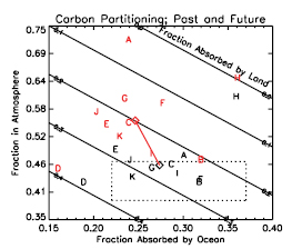
Figure 7.13. Predicted increase in the fraction of total emissions that add to atmospheric CO2.Changes in the mean partitioning of emissions as simulated by theC4MIP models up to 2000 (black symbols) and for the entire simulation period to 2100 (red symbols). The letters represent the models as given in Table 7.4 .The box shown by the dotted line is a constraint on the historical carbon balance based on records of atmospheric CO2 increase, and estimates of total emissions (fossil fuel plus land use emissions) and the oceanic uptake of anthropogenic CO2 ( Sabine et al., 2004a [JoC, SRC] ). The black and red diamonds show the model-mean carbon partitioning for the historical period and the entire simulation period, respectively. The red line shows the mean tendency towards an increasing airborne fraction through the 21st century, which is common to all models.
7.3.5.3 Sensitivity Analysis
The coupled and uncoupled model experiments can be used to separate the effects of climate change and CO2 increase on land and ocean carbon storage ( Friedlingstein et al., 2003 [JoC, SRC] ). Table 7.4 also shows the linear sensitivity parameters diagnosed from each of theC4MIP models ( Friedlingstein et al., 2006 [JoC, MoS, SRC] ).
7.3.5.3.1 Increase in ocean carbon uptake with increasing atmospheric carbon dioxide
The ocean takes up CO2 at a rate that depends on the difference between pCO2 in the atmosphere and in the surface ocean. Model estimates of uptake differ primarily because of differences in the rate at which carbon is exported from the surface ocean to depth by the large-scale circulation ( Doney et al., 2004 [JoC, MoS] ; Section 7.3.4.1 ; Box 7.3 )and the biological pump ( Sarmiento et al., 2004 [JoC] ). Ocean carbon cycle model intercomparisons have shown that the simulated circulation in the Southern Ocean can have a large impact on the efficiency with which CO2,and other anthropogenic tracers such as CFCs, are drawn down ( Orr et al., 2001 [JoC, MoS, ARC] ; Dutay et al., 2002 [JoC, MoS] ). TheC4MIP models show ocean carbon storage increases ranging from 0.9 to 1.6 GtC ppm–1,which is equivalent to ocean uptake increasing at between 42 and 75% of the rate of atmospheric CO2 increase. Basic ocean carbonate chemistry suggests that the ocean-borne fraction of emissions will fall in the future, even in the absence of climate change, because of an increasing ocean buffer factor( Section 7.3.4.2 ).
7.3.5.3.2 Increase in land carbon uptake with increasing atmospheric carbon dioxide
In the absence of land use change and forest fires, land carbon storage depends on the balance between the input of carbon as NPP, and the loss of carbon as heterotrophic (soil) respiration( Section 7.3.3 ). There is an ongoing debate concerning the importance of CO2 fertilization at the patch scale where other constraints such as N limitation may dominate; recent surveys indicate a wide range of possible responses to a CO2 increase of around 50%, with average increases of 12 to 23% ( Norby et al., 2005 [JoC] ; see Section 7.3.3.1 ).
TheC4MIP models show increases in global NPP of between 6 and 33% when CO2 increases over the same range. These figures are not directly comparable: someC4MIP models include vegetation dynamics, which are likely to increase the vegetation cover as well as the NPP per unit of vegetation area, and therefore lead to higher overall sensitivity of global NPP to CO2.The FACE experiments also typically involve an instantaneous increase in CO2.However, mostC4MIP models are within the range of the CO2 sensitivities measured.
The overall response of land carbon storage to CO2 is given by the fifth column of Table 7.4 .TheC4MIP models show time-mean land carbon storage increases ranging from 0.2 to 2.5 GtC ppm–1,with all but two models between 1.1 and 1.6 GtC ppm–1.This response is driven by the CO2 fertilization of NPP in each model, with a counteracting tendency for the mean soil carbon turnover rate (i.e., the heterotrophic respiration by unit soil carbon) to increase even in the absence of climate change. This somewhat surprising effect of CO2 is seen to varying degrees in allC4MIP models. It appears to arise because CO2 fertilization of NPP acts particularly to increase vegetation carbon, and therefore litter fall and soil carbon, in productive tropical regions that have high intrinsic decomposition rates. This increases the average turnover rate of the global soil carbon pool even though local turnover rates are unchanged. In some models (e.g., model C) this acts to offset a significant fraction of the land carbon increase arising from CO2 fertilization. Models with large responses of ocean or land carbon storage to CO2 tend to have weaker climate-carbon cycle feedbacks because a significant fraction of any carbon released through climate change effects is reabsorbed through direct CO2 effects ( Thompson et al., 2004 [JoC, MoS] ).
7.3.5.3.3 Transient climate sensitivity to carbon dioxide
The strength of the climate-carbon cycle feedback loop depends on both the sensitivity of the carbon cycle to climate, and the sensitivity of climate to CO2.The equilibrium climate sensitivity to a doubling of atmospheric CO2 concentration remains a critical uncertainty in projections of future climate change, but also has a significant bearing on future CO2 concentrations, with higher climate sensitivities leading to larger climate-carbon cycle feedbacks ( Andreae et al., 2005 [JoC, MoS, SRC] ). The fourth column of Table 7.4 shows the transient global climate sensitivity (i.e., the global climate warming that results when the transient simulation passes doubled atmospheric CO2)for each of theC4MIP models. All but two models (models E and I) have transient climate sensitivities in the range 1.9°C to 2.7°C. However, differences in carbon cycle responses are likely to occur because of potentially large differences in regional climate change, especially where this affects water availability on the land.
7.3.5.3.4 Dependence of ocean carbon uptake on climate.
Climate change can reduce ocean uptake through reductions in CO2 solubility, suppression of vertical mixing by thermal stratification and decreases in surface salinity. On longer time scales (>70 years) the ocean carbon sink may also be affected by climate-driven changes in large-scale circulation (e.g., a slowing down of the thermohaline circulation). The last column of Table 7.4 shows the sensitivity of ocean carbon storage to climate change as diagnosed from theC4MIP models. All models indicate a reduction in the ocean carbon sink by climate change of between –14 and –60 GtC °C–1,implying a positive climate-CO2 feedback.
7.3.5.3.5 Dependence of land carbon storage on climate.
The major land-atmosphere fluxes of CO2 are strongly climate dependent. Heterotrophic respiration and NPP are both very sensitive to water availability and ambient temperatures. Changes in water availability depend critically on uncertain regional aspects of climate change projections and are therefore likely to remain a dominant source of uncertainty (see Chapter 11 ). The overall sensitivity of land carbon storage to climate( Table 7.4 ,seventh column) is negative in all models, implying a positive climate-CO2 feedback, but the range is large: –19 to –175 GtC °C–1.These values are determined by the combined effects of climate change on NPP and the soil carbon turnover (or decomposition) rate, as shown in Table 7.5 .
TheC4MIP models utilise different representations of soil carbon turnover, ranging from single-pool models (model A) to nine-pool models (model E). However, most soil models assume a similar acceleration of decay with temperature, approximately equivalent to a doubling of the specific respiration rate for every 10°C warming. This temperature sensitivity is broadly consistent with a long history of lab and field measurements of soil efflux ( Raich and Schlesinger, 1992 [JoC] ), although there is an ongoing difficulty in separating root and soil respiration. Note, however, that the expected dependence on temperature was not found at the whole ecosystem level for decadal time scales, in forest soils ( Giardina and Ryan, 2000 [JoC] ; Melillo et al., 2002 [JoC] ), grasslands ( Luo et al., 2001 [JoC, ARC] ) or boreal forests ( Dunn et al., 2007 [2007] ). These apparent discrepancies may reflect the rapid depletion of labile pools of organic matter, with strong temperature responses likely so long as litter inputs are maintained ( Knorr et al., 2005 [JoC, SRC] ). Nevertheless, the temperature sensitivity of the slow carbon pools is still poorly known.
Table 7.5 shows that allC4MIP models simulate an overall increase in soil carbon turnover rate as the climate warms, ranging from 2 to 10% per °C. The use of a single soil carbon pool in the Hadley model (A) cannot completely account for the relatively large sensitivity of soil respiration to temperature in this model ( Jones et al., 2005 [MoS, SRC] ), as evidenced by the lower effective sensitivity diagnosed from the UVic model (model G), which uses the same soil-vegetation component. It seems more likely that differences in soil moisture simulations are playing the key part in determining the effective sensitivity of soil turnover rate to climate. Table 7.5 also shows the effective sensitivities of NPP to climate, ranging from a significant reduction of 6% per °C to smaller climate-change driven increases of 2% per °C under climate change. This variation may reflect different time scales for boreal forest response to warming (leading to a positive impact on global NPP), as well as different regional patterns of climate change ( Fung et al., 2005 [JoC, SRC] ). The models with the largest negative responses of NPP to climate (models A, B and C) also show the tendency for tropical regions to dry under climate change, in some cases significantly ( Cox et al., 2004 [MoS, SRC] ).
Table 7.5. Effective sensitivities of land processes in theC4MIP models: percent change of vegetation NPP to a doubling of atmospheric CO2 concentration (Column 2), and sensitivities of vegetation NPP and specific heterotrophic soil respiration to a 1°C global temperature increase (Columns 3 and 4).
| Modela | Sensitivity of Vegetation NPP to CO2: | Sensitivity of Vegetation NPP to Climate: | Sensitivity of Specific Heterotrophic Respiration Rate to Climate: |
|---|---|---|---|
| %change for a CO2 doubling | %change for a 1°C increase | %change for a 1°C increase | |
| A. HadCM3LC | 57 | –5.8 | 10.2 |
| B. IPSL-CM2C | 50 | –4.5 | 2.3 |
| C. MPI-M | 76 | –4.0 | 2.8 |
| D. LLNL | 73 | –0.4 | 7.0 |
| E. NCAR CSM-1 | 34 | 0.8 | 6.2 |
| F. FRCGC | 21 | 1.2 | 7.2 |
| G. UVic-2.7 | 47 | –2.3 | 6.5 |
| H. UMC | 12 | –1.6 | 4.8 |
| I. BERN-CC | 46 | 1.2 | 8.7 |
| J. CLIMBER2-LPJ | 44 | 1.9 | 9.4 |
| K. IPSL-CM4-LOOP | 64 | –0.3 | 2.9 |
| Mean | 48 | –1.3 | 6.2 |
| Std Dev | ±20 | ±2.6 | ±2.7 |
7.3.5.4 Summary of Coupling Between the Carbon Cycle and Climate
7.3.5.4.1 Robust findings
Results from the coupled climate-carbon cycle models participating in theC4MIP project support the following statements:
• AllC4MIP models project an increase in the airborne fraction of total anthropogenic CO2 emissions through the 21st century.
• The CO2 increase alone will lead to continued uptake by the land and the ocean, although the efficiency of this uptake will decrease through the carbonate buffering mechanism in the ocean, and through saturation of the land carbon sink.
• Climate change alone will tend to suppress both land and ocean carbon uptake, increasing the fraction of anthropogenic CO2 emissions that remain airborne and producing a positive feedback to climate change. The magnitude of this feedback varies among theC4MIP models, ranging from a 4 to 44% increase in the rate of increase of CO2,with a mean (± standard deviation) of 18 ± 11%.
7.3.5.4.2 Key uncertainties
TheC4MIP models also exhibit uncertainties in the evolution of atmospheric CO2 for a given anthropogenic emissions scenario. Figure 7.14 shows how uncertainties in the sensitivities of ocean and land carbon processes contribute to uncertainties in the fraction of emissions that remain in the atmosphere. The confidence limits were produced by spanning the range of sensitivities diagnosed from the 11C4MIP models (Tables 7.4 and 7.5 ). In the absence of climate change effects (lowest three bars), models simulate increased uptake by ocean and land (primarily as a result of CO2 enhancement of NPP), with a slight offset of the land uptake by enhancement of the specific heterotrophic respiration rate (see Section 7.3.5.3.2 ). However, there is a wide range of response to CO2,even in the absence of climate change effects on the carbon cycle. Climate change increases the fraction of emissions that remain airborne by suppressing ocean uptake, enhancing soil respiration and reducing plant NPP. The sensitivity of NPP to climate change is especially uncertain because it depends on changing soil water availability, which varies significantly between General Circulation Models (GCMs), with some models suggesting major drying and reduced productivity in tropical ecosystems ( Cox et al., 2004 [MoS, SRC] ). The transient climate sensitivity to CO2 is also a major contributor to the overall uncertainty in the climate-carbon cycle feedback (top bar).
Other potentially important climate-carbon cycle interactions were not included in these first generationC4MIP experiments. The ocean ecosystem models used inC4MIP are at an early stage of development. These models have simple representations of the biological fluxes, which include the fundamental response to changes in internal nutrients, temperature and light availability, but for most models do not include the more complex responses to changes in ecosystem structure. Changes in ecosystem structure can occur when specific organisms respond to surface warming, acidification, changes in nutrient ratios resulting from changes in external sources of nutrients (atmosphere or rivers) and changes in upper trophic levels (fisheries). Shifts in the structure of ocean ecosystems can influence the rate of CO2 uptake by the ocean ( Bopp et al., 2005 [JoC, MoS] ).
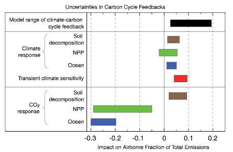
Figure 7.14. Uncertainties in carbon cycle feedbacks estimated from analysis of the results from theC4MIP models. Each effect is given in terms of its impact on the mean airborne fraction over the simulation period (typically 1860 to 2100 ), with bars showing the uncertainty range based on the ranges of effective sensitivity parameters given in Tables 7.4 and 7.5 .The lower three bars are the direct response to increasing atmospheric CO2 (see Section 7.3.5 for details), the middle four bars show the impacts of climate change on the carbon cycle, and the top black bar shows the range of climate-carbon cycle feedbacks given by theC4MIP models.
The first-generationC4MIP models also currently exclude, by design, the effects of forest fires and prior land use change. Forest regrowth may account for a large part of the land carbon sink in some regions (e.g., Pacala et al., 2001 [JoC, MoS] ; Schimel et al., 2001 [JoC] ; Hurtt et al., 2002 [JoC, MoS] ; Sitch et al., 2005 [JoC, MoS] ), while combustion of vegetation and soil organic matter may be responsible for a significant fraction of the interannual variability in CO2 ( Cochrane, 2003 [JoC] ;( Nepstad et al., 2004; ) Kasischke et al., 2005 [JoC] ; Randerson et al., 2005 [JoC] ). Other important processes were excluded in part because modelling these processes is even less straightforward. Among these are N cycling on the land (which could enhance or suppress CO2 uptake by plants) and the impacts of increasing ozone concentrations on plants (which could suppress CO2 uptake).
7.4 Reactive Gases and the Climate System
The atmospheric concentration of many reactive gases has increased substantially during the industrial era as a result of human activities. Some of these compounds (CH4,N2O, halocarbons, ozone, etc.) interact with longwave (infrared) solar radiation and, as a result, contribute to ‘greenhouse warming’. Ozone also efficiently absorbs shortwave (ultraviolet and visible) solar energy, so that it protects the biosphere (including humans) from harmful radiation and plays a key role in the energy budget of the middle atmosphere. Many atmospheric chemical species are emitted at the surface as a result of biological processes (soils, vegetation, oceans) or anthropogenic activities (fossil fuel consumption, land use changes) before being photochemically destroyed in the atmosphere and converted to compounds that are eventually removed by wet and dry deposition. The oxidizing power (or capacity) of the atmosphere is determined primarily by the atmospheric concentration of the OH radical (daytime) and to a lesser extent the concentrations of the nitrate radical (NO3;nighttime), ozone and hydrogen peroxide (H2O2). The coupling between chemical processes in the atmosphere and the climate system( Figure 7.15 )are complex because they involve a large number of physical, chemical and biological processes that are not always very well quantified. An important issue is to determine to what extent predicted climate change could affect air quality (see Box 7.4 ). The goal of this section is assess recent progress made in the understanding of the two-way interactions between reactive gases and the climate system.
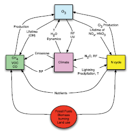
Figure 7.15. Schematic representation of the multiple interactions between tropospheric chemical processes, biogeochemical cycles and the climate system. RF represents radiative forcing, UV ultraviolet radiation, T temperature and HNO3 nitric acid.
Box 7.4: Effects of Climate Change on Air Quality
Weather is a key variable affecting air quality. Surface air concentrations of pollutants are highly sensitive to boundary layer ventilation, winds, temperature, humidity and precipitation. Anomalously hot and stagnant conditions in the summer of 1988 were responsible for the highest ozone year on record in the north-eastern USA ( Lin et al., 2001 [SRC] ). The summer heat wave in Europe in 2003 was associated with exceptionally high ozone ( (Ordonez et al., 2005 ) ). Such high interannual variability of surface ozone correlated with temperature demonstrates the potential air quality implications of climate change over the next century.
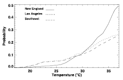
Box 7.4 ,Figure 1. Probability that the daily maximum eight-hour average ozone concentration will exceed the US National Ambient Air Quality Standard of 0.08 ppm for a given daily maximum temperature based on 1980 to 1998 data. Values are shown for New England (bounded by 36°N, 44°N, 67.5°W and 87.5°W), the Los Angeles Basin (bounded by 32°N, 40°N, 112.5°W and 122.5°W) and the southeastern USA (bounded by 32°N, 36°N, 72.5°W and 92.5°W). Redrawn from Lin et al. 2001 [SRC] ).
Afew GCM studies have investigated how air pollution meteorology might respond to future climate change. Rind et al. 2001 [JoC, ARC] ) found that increased continental ventilation as a result of more vigorous convection should decrease surface concentrations, while Holzer and Boer 2001 [JoC, MoS] ) found that weaker winds should result in slower dilution of pollution plumes and hence higher concentrations. A focused study by Mickley et al. 2004 [JoC, MoS, SRC] ) for the eastern USA found an increase in the severity and persistence of regional pollution episodes due to the reduced frequency of ventilation by cyclones tracking across Canada. This effect more than offsets the dilution associated with the small rise in mixing depths. A decrease in cyclone frequency at northern mid-latitudes and a shift to higher latitudes has been noted in observations from the past few decades ( McCabe et al., 2001 [JoC] ). An urban air quality model study by Jacobson 1999 [JoC] ) pointed out that decreasing soil moisture or increasing surface temperature would decrease mixing depths and reduce near-surface pollutant concentrations.
Anumber of studies in the USA have shown that summer daytime ozone concentrations correlate strongly with temperature ( NRC, 1991 [NPR] ). This correlation appears to reflect contributions of comparable magnitude from (1) temperature-dependent biogenic VOC emissions, (2) thermal decomposition of peroxyacetylnitrate, which acts as a reservoir for NOx and (3) association of high temperatures with regional stagnation ( Jacob et al., 1993 [JoC, SRC] ; Sillman and Samson, 1995 [JoC] ; Hauglustaine et al., 2005 [JoC, MoS, SRC] ). Empirical relationships between ozone air quality standard exceedances and temperature, as shown in Figure 1, integrate all of these effects and could be used to estimate how future regional changes in temperature would affect ozone air quality. Changes in the global ozone background would also have to be accounted for ( Stevenson et al., 2005 [NPR, SRC] ).
Afew GCM studies have examined more specifically the effect of changing climate on regional ozone air quality, assuming constant emissions. ( Knowlton et al. 2004 ) ) use a GCM coupled to a Regional Climate Model (RCM) to investigate the impact of 2050 climate change (compared with 1990 ) on ozone concentrations in the New York City metropolitan area. They found a significant ozone increase that they translated into a 4.5% increase in ozone-related acute mortality. ( Langner et al. 2005 ) ) use an RCM driven by two different GCMs to examine changes in the Accumulated Ozone concentration above a Threshold of 40 ppb (AOT40) statistic (ozone-hours above 40 ppb) over Europe in 2050 to 2070 relative to the present. They found an increase in southern and central Europe and a decrease in northern Europe that they attributed to different regional trends in cloudiness and precipitation. Dentener et al. 2006 [SRC] ) synthesise the results of 10 global model simulations for 2030 driven by future compared with present climate. They find that climate change caused mean decreases in surface ozone of 0.5 to 1 ppb over continents and 1 to 2 ppb over the oceans, although some continental regions such as the Eastern USA experienced slight increases.
There has been less work on the sensitivity of aerosols to meteorological conditions. Regional model simulations by Aw and Kleeman 2003 [JoC] ) find that increasing temperatures should increase surface aerosol concentrations due to increased production of aerosol precursors (in particular semi-volatile organic compounds and HNO3)although this is partly compensated by the increasing vapour pressure of these compounds at higher temperatures. Perturbations of precipitation frequencies and patterns might be expected to have a major impact on aerosol concentrations, but the GCM study by Mickley et al. 2004 [JoC, MoS, SRC] ) for 2000 to 2050 climate change finds little effect in the USA.
7.4.1 Methane
7.4.1.1 Biogeochemistry and Budgets of Methane
Atmospheric CH4 originates from both non-biogenic and biogenic sources. Non-biogenic CH4 includes emissions from fossil fuel mining and burning (natural gas, petroleum and coal), biomass burning, waste treatment and geological sources (fossil CH4 from natural gas seepage in sedimentary basins and geothermal/volcanic CH4). However, emissions from biogenic sources account for more than 70% of the global total. These sources include wetlands, rice agriculture, livestock, landfills, forests, oceans and termites. Emissions of CH4 from most of these sources involve ecosystem processes that result from complex sequences of events beginning with primary fermentation of organic macromolecules to acetic acid (CH3COOH), other carboxylic acids, alcohols, CO2 and hydrogen (H2), followed by secondary fermentation of the alcohols and carboxylic acids to acetate,H2 and CO2,which are finally converted to CH4 by the so-called methanogenic Archaea: CH3COOH → CH4 +CO2 and CO2 +4H2 → CH4 +2H2O(Conrad, 1996 ). Alternatively, CH4 sources can be divided into anthropogenic and natural. The anthropogenic sources include rice agriculture, livestock, landfills and waste treatment, some biomass burning, and fossil fuel combustion. Natural CH4 is emitted from sources such as wetlands, oceans, forests, fire, termites and geological sources( Table 7.6 ).
The net rate of CH4 emissions is generally estimated from three approaches: (1) extrapolation from direct flux measurements and observations, (2) process-based modelling (bottom-up approach) and (3) inverse modelling that relies on spatially distributed, temporally continuous observations of concentration, and in some cases isotopic composition in the atmosphere (top-down approach). The top-down method also includes aircraft and satellite observations ( Xiao et al., 2004 [NPR, JoC] ; Frankenberg et al., 2005 [JoC] , 2006 ). When the bottom-up approach is used to extrapolate the emissions to larger scales, uncertainty results from the inherent large temporal and spatial variations of fluxes and the limited range of observational conditions. The top-down approach helps to overcome the weaknesses in bottom-up methods. However, obstacles to extensive application of the top-down approach include inadequate observations, and insufficient capabilities of the models to account for error amplification in the inversion process and to simulate complex topography and meteorology ( Dentener et al., 2003a [JoC, SRC] ; Mikaloff Fletcher et al., 2004a [JoC, MoS] , 2004b; Chen and Prinn, 2005 [JoC, MoS, ARC] , 2006 ). Measurements of isotopes of CH4 (13C, 14C, and 2H) provide additional constraints on CH4 budgets and specific sources, but such data are even more limited ( Bergamaschi et al., 2000 [JoC] ; Lassey et al., 2000 [JoC, SRC] ; Mikaloff Fletcher et al., 2004a [JoC, MoS] , 2004b ).
Since the TAR, availability of new data from various measurement networks and from national reporting documents has enabled re-estimates of CH4 source magnitudes and insights into individual source strengths. Total global pre-industrial emissions of CH4 are estimated to be 200 to 250 Tg(CH4)yr–1 ( Chappellaz et al., 1993 [JoC, SRC] ; Etheridge et al., 1998 [JoC, ARC] ; Houweling et al., 2000 [JoC, MoS, SRC] ; Ferretti et al., 2005 [JoC] ; Valdes et al., 2005 [NPR, JoC] ). Of this, natural CH4 sources emitted between 190 and 220 Tg(CH4)yr–1,and anthropogenic sources (rice agriculture, livestock, biomass burning and waste) accounted for the rest ( Houweling et al., 2000 [JoC, MoS, SRC] ; Ruddiman and Thomson, 2001 [JoC] ). In contrast, anthropogenic emissions dominate present-day CH4 budgets, accounting for more than 60% of the total global budget( Table 7.6 ).
The single largest CH4 source is natural wetlands. Recent estimates combine bottom-up and top-down fluxes, and global observations of atmospheric CH4 concentrations in a three-dimensional Atmospheric Transport and Chemical Model (ATCM) simulation ( Chen and Prinn, 2005 [JoC, MoS, ARC] , 2006 ). In these estimates, southern and tropical regions account for more than 70% of total global wetland emissions. Other top-down studies that include both direct observations and 13C/12Cratios of CH4 suggest greater emissions in tropical regions compared with previously estimates ( Mikaloff Fletcher et al., 2004a [JoC, MoS] , 2004b; Xiao et al., 2004 [NPR, JoC] ; Frankenberg et al., 2006 [NPR, JoC] ). However, several bottom-up studies indicate fewer emissions from tropical rice agriculture ( Li et al., 2002 [NPR, JoC] ; Yan et al., 2003 [MoS] ;( Khalil and Shearer 2006 ) Frankenberg et al. 2005 [JoC] , 2006 and Keppler et al. 2006 [JoC] ) suggest that tropical trees emit CH4 via an unidentified process. The first estimate of this source was 10 to 30% (62–236 Tg(CH4)yr–1)of the global total, but ( Kirschbaum et al. 2006 ) ) revise this estimate downwards to 10 to 60 Tg(CH4)yr–1.Representative 13C/12Cratios (δ13Cvalues) of CH4 emitted from individual sources are included in Table 7.6 .Due to isotope fractionation associated with CH4 production and consumption processes, CH4 emitted from each source exhibits a measurably different δ13Cvalue. Therefore, it is possible, using mixing models, to constrain further the sources of atmospheric CH4.
Geological sources of CH4 are not included in Table 7.6 .However, several studies suggest that significant amounts of CH4,produced within the Earth’s crust (mainly by bacterial and thermogenic processes), are released into the atmosphere through faults and fractured rocks, mud volcanoes on land and the seafloor, submarine gas seepage, microseepage over dry lands and geothermal seeps ( (Etiope and Klusman, 2002; ) ( Etiope, 2004; ) ( Kvenvolden and Rogers, 2005 ) ). Emissions from these sources are estimated to be as large as 40 to 60 Tg(CH4)yr–1.
Table 7.6 Sources, sinks and atmospheric budgets of CH4 (Tg(CH4)yr–1).a
| References | Indicative 13C, ‰b | Hein et al., 1997c | Houweling et al., 2000c | Olivier et al., 2005 | Wuebbles and Hayhoe, 2002 | Scheehle et al., 2002 | J. Wang et al., 2004c | Mikaloff Fletcher et al., 2004ac | Chen and Prinn, 2006c | TAR | AR4 |
|---|---|---|---|---|---|---|---|---|---|---|---|
| Base year | 1983–1989 | 2000 | 1990 | 1994 | 1999 | 1996–2001 | 1998 | 2000–2004 | |||
| Natural sources | 222 | 145 | 200 | 260 | 168 | ||||||
| Wetlands | –58 | 231 | 163 | 100 | 176 | 231 | 145 | ||||
| Termites | –70 | 20 | 20 | 20 | 29 | 23 | |||||
| Ocean | –60 | 15 | 4 | ||||||||
| Hydrates | –60 | 5 | 4 | ||||||||
| Geological sources | –40 | 4 | 14 | ||||||||
| Wild animals | –60 | 15 | |||||||||
| Wildfires | –25 | 5 | 2 | ||||||||
| Anthropogenic sources | 361 | 320 | 358 | 264 | 307 | 350 | 428 | ||||
| Energy | 74 | 77 | |||||||||
| Coal mining | –37 | 32 | 34 | 46 | 30 | 48d | |||||
| Gas, oil, industry | –44 | 68 | 64 | 60 | 52 | 36e | |||||
| Landfills & waste | –55 | 43 | 66 | 61 | 69 | 49 | 35 | ||||
| Ruminants | –60 | 92 | 80 | 81 | 76 | 83 | 91 | 189f | |||
| Rice agriculture | –63 | 83 | 39 | 60 | 31 | 57 | 54 | 112 | |||
| Biomass burning | –25 | 43 | 50 | 14 | 41 | 88 | 43e | ||||
| C3 vegetation | –25 | 27 | |||||||||
| C4 vegetation | –12 | 9 | |||||||||
| Total sources | 592 | 503 | 507 | 610 | 596 | 598 | 582 | ||||
| Imbalance | +33 | +22 | +1 | ||||||||
| Sinks | |||||||||||
| Soils | –18 | 26 | 30 | 34 | 30 | 30 | 30g | ||||
| Tropospheric OH | –3.9 | 488 | 445 | 428 | 507 | 506 | 511g | ||||
| Stratospheric loss | 45 | 40 | 30 | 40 | 40 | 40g | |||||
| Total sink | 559 | 515 | 492 | 577 | 576 | 581g |
The major CH4 sinks are oxidation by OH in the troposphere, biological CH4 oxidation in drier soil, and loss to the stratosphere( Table 7.6 ). Oxidation by chlorine (Cl) atoms in the marine atmospheric boundary layer is suggested as an additional sink for CH4,possibly constituting an additional loss of about 19 Tg(CH4)yr–1 ( Gupta et al., 1997 [JoC] ; Tyler et al., 2000 [JoC] ; Platt et al., 2004 [ARC] ; Allan et al., 2005 [JoC] ). However, the decline in the growth rate of atmospheric CH4 concentration since the TAR shows no clear correlation with change in sink strengths over the same period ( Prinn et al., 2001 [JoC, ARC] , 2005; Allan et al., 2005 [JoC] ). This trend has continued since 1993, and the reduction in the CH4 growth rate has been suggested to be a consequence of source stabilisation and the approach of the global CH4 budget towards steady state ( Dlugokencky et al., 1998 [JoC, SRC] , 2003 ). Thus, total emissions are likely not increasing but partitioning among the different sources may have changed (see Section 2.3 ). Consequently, in the Fourth Assessment Report (AR4) the sink strength is treated as in the TAR (576 Tg(CH4)yr–1). However, the AR4 estimate has been increased by 1% (to 581 Tg(CH4)yr–1)to take into account the recalibration of the CH4 scale explained in Chapter2 .The main difference between TAR and AR4 estimates is the source-sink imbalance inferred from the annual increment in concentration. The TAR used 8 ppb yr–1 for a period centred on 1998 when there was clearly an anomalously high growth rate. The present assessment uses 0.2 ppb yr–1,the average over 2000 to 2005 (see Section 2.3 and Figure 2.4 ). Thus, using the CH4 growth rate for a single anomalous year, as in the TAR, gives an anomalously high top-down value relative to the longer-term average source. For a conversion factor of 2.78 Tg(CH4)per ppb and an atmospheric concentration of 1,774 ppb, the atmospheric burden of CH4 in 2005 was 4,932 Tg, with an annual average increase ( 2000 – 2005 ) of about 0.6 Tg yr–1.Total average annual emissions during the period considered here are approximately 582 Tg(CH4)yr–1.
Uncertainty in this estimate may arise from several sources. Uncertainty in the atmospheric concentration measurement, given in Chapter2 as 1,774 ± 1.8 ppb in 2005, is small (about 0.1%). Uncertainty ranges for individual sink estimates are ±103 Tg(CH4)(20%), ±15 Tg(CH4)(50%), ±8 Tg(CH4)(20%) for OH, soil and stratospheric loss, respectively (as reported in the Second Assessment Report). The use of a different lifetime for CH4 (8.7 ± 1.3 years) leads to an uncertainty in overall sink strength of ±15%. Thus, the top-down method used in AR4 is constrained mainly by uncertainty in sink estimates and the choice of lifetime used in the mass balance calculation.
7.4.1.2 Effects of Climate
Effects of climate on CH4 biogeochemistry are investigated by examining records of the past and from model simulations under various climate change scenarios. Ice core records going back 650 ka ( Petit et al., 1999 [JoC] ; Spahni et al., 2005 [JoC, ARC] ) reveal that the atmospheric concentration of CH4 is closely tied to atmospheric temperature, falling and rising in phase with temperature at the inception and termination of glacial episodes ( (Wuebbles and Hayhoe, 2002 ) Brook et al. 2000 [JoC] ) show that, following each transition, temperature increased more rapidly than CH4 concentration. Since biogenic CH4 production and emission from major sources (wetlands, landfills, rice agriculture and biomass burning) are influenced by climate variables such as temperature and moisture, the effect of climate on emissions from these sources is significant.
Several studies indicate a high sensitivity of wetland CH4 emissions to temperature and water table. Before the 1990 s, elevated surface temperature and emissions from wetlands were believed to contribute to the increase in global CH4 emissions ( Walter and Heimann, 2001a [JoC, MoS, SRC] ,b; Christensen et al., 2003 [JoC] ; Zhuang et al., 2004 [NPR, JoC, MoS] ). Observations indicate substantial increases in CH4 released from northern peatlands that are experiencing permafrost melt ( Christensen et al., 2004 [NPR, JoC] ; Wickland et al., 2006 [JoC] ). Based on the relationship between emissions and temperature at two wetland sites in Scotland, ( Chapman and Thurlow 1996 ) ) predicted that CH4 emissions would increase by 17, 30 and 60% for warmings of 1.5°C, 2.5°C and 4.5°C (warming above the site’s mean temperature during 1951 to 1980 ), respectively. A model simulation by ( Cao et al. 1998 ) ) yielded a 19% emission increase under a uniform 2°C warming. The combined effects of a 2°C warming and a 10% increase in precipitation yielded an increase of 21% in emissions. In most cases, the net emission depends on how an increase in temperature affects net ecosystem production (NEP), as this is the source of methanogenic substrates ( Christensen et al., 2003 [JoC] ), and on the moisture regime of wetlands, which determines if decomposition is aerobic or anaerobic. Emissions increase under a scenario where an increase in temperature is associated with increases in precipitation and NEP, but emissions decrease if elevated temperature results in either reduced precipitation or reduced NEP.
For a doubling in atmospheric CO2 concentration, the GCM of Shindell et al. 2004 [JoC] ) simulates a 3.4°C warming. Changes in the hydrological cycle due to this CO2 doubling cause CH4 emissions from wetlands to increase by 78%. Gedney et al. 2004 [JoC, SRC] ) also simulate an increase in CH4 emissions from northern wetlands due to an increase in wetland area and an increase in CH4 production due to higher temperatures. Zhuang et al. 2004 [NPR, JoC, MoS] ) use a terrestrial ecosystem model based on emission data for the 1990 s to study how rates of CH4 emission and consumption in high-latitude soils of the NH (north of 45°N) have changed over the past century ( 1900 – 2000 ) in response to observed change in the region’s climate. They estimate that average net emissions of CH4 increased by 0.08 Tg yr–1 over the 20th century. Their decadal net CH4 emission rate correlates with soil temperature and water table depth.
In rice agriculture, climate factors that will likely influence CH4 emission are those associated with plant growth. Plant growth controls net emissions by determining how much substrate will be available for either methanogenesis or methanotrophy ( Matthews and Wassmann, 2003 [MoS] ( Sass et al. 2002 ) ) show that CH4 emissions correlate strongly with plant growth (height) in a Texas rice field. Any climate change scenario that results in an increase in plant biomass in rice agriculture is likely to increase CH4 emissions ( (Xu et al., 2004 ) ). However, the magnitude of increased emission depends largely on water management. For example, field drainage could significantly reduce emission due to aeration of the soil (i.e., influx of air into anaerobic zones that subsequently suppresses methanogenesis, Li et al., 2002 [NPR, JoC] ).
Past observations indicate large interannual variations in CH4 growth rates ( Dlugokencky et al., 2001 [JoC, ARC] ). The mechanisms causing these variations are poorly understood and the role of climate is not well known. Emissions from wetlands and biomass burning may have contributed to emission peaks in 1993 to 1994 and 1997 to 1998 ( Langenfelds et al., 2002 [JoC] ; Butler et al., 2004 [MoS, SRC] ). Unusually warm and dry conditions in the NH during ENSO periods increase biomass burning. Kasischke and Bruhwiler 2002 [JoC] ) attribute CH4 releases of 3 to 5 Tg in 1998 to boreal forest fires in Eastern Siberia resulting from unusually warm and dry conditions.
Meteorological conditions can affect global mean removal rates ( Warwick et al., 2002 [JoC] ; Dentener et al., 2003a [JoC, SRC] ). Dentener et al. find that over the period 1979 to 1993, the primary effect resulted from changes in OH distribution caused by variations in tropical tropospheric water vapour. Johnson et al. 2001 [JoC, MoS, SRC] ) studied predictions of the CH4 evolution over the 21st century and found that there is also a substantial increase in CH4 destruction due to increases in the CH4 + OH rate coefficient in a warming climate. There also appear to be significant interannual variations in the active Cl sink, but a climate influence has yet to be identified ( Allan et al., 2005 [JoC] ). On the other hand, several model studies indicate that CH4 oxidation in soil is relatively insensitive to temperature increase (Ridgwell at al., 1999; Zhuang et al., 2004 [NPR, JoC, MoS] ). A doubling of atmospheric CO2 would likely change the sink strength only marginally (in the range of –1 to +3 Tg(CH4)yr–1 ;Ridgwell et al., 1999 [JoC, MoS] ). However, any change in climate that alters the amount and pattern of precipitation may significantly affect the CH4 oxidation capacity of soils. A process-based model simulation indicated that CH4 oxidation strongly depends on soil gas diffusivity, which is a function of soil bulk density and soil moisture content ( Bogner et al., 2000 [JoC, MoS] ; del Grosso et al., 2000 [JoC, MoS] ).
Climate also affects the stability of CH4 hydrates beneath the ocean, where large amounts of CH4 are stored (~4 ×10⁶ Tg; Buffett and Archer, 2004 [SRC] ). The δ13Cvalues of ancient seafloor carbonates reveal several hydrate dissociation events that appear to have occurred in connection with rapid warming episodes in the Earth’s history ( Dickens et al., 1997 [MoS] ; Dickens, 2001 [NPR, MoS] ). Model results indicate that these hydrate decomposition events occurred too fast to be controlled by the propagation of the temperature change into the sediments ( Katz et al., 1999 [JoC] ;( Paull et al., 2003 ) ). Additional studies infer other indirect and inherently more rapid mechanisms such as enhanced migration of free gas, or reordering of gas hydrates due to slump slides ( Hesselbo et al., 2000 [JoC] ;( Jahren et al., 2001; ) ( Kirschvink et al., 2003; ) ( Ryskin, 2003 ) ). Recent modelling suggests that today’s seafloor CH4 inventory would be diminished by 85% with a warming of bottom water temperatures by 3°C ( Buffett and Archer, 2004 [SRC] ). Based on this inventory, the time-dependent feedback of hydrate destabilisation to global warming has been addressed using different assumptions for the time constant of destabilisation: an anthropogenic release of 2,000 GtC to the atmosphere could cause an additional release of CH4 from gas hydrates of a similar magnitude (∼2,000 Gt(CH4)) over a period of 1 to 100 kyr ( Archer and Buffett, 2005 [MoS, SRC] ). Thus, gas hydrate decomposition represents an important positive CH4 feedback to be considered in global warming scenarios on longer time scales.
In summary, advances have been made since the TAR in constraining estimates of CH4 source strengths and in understanding emission variations. These improvements are attributed to increasing availability of worldwide observations and improved modelling techniques. Emissions from anthropogenic sources remain the major contributor to atmospheric CH4 budgets. Global emissions are likely not to have increased since the time of the TAR, as nearly zero growth rates in atmospheric CH4 concentrations have been observed with no significant change in the sink strengths.
7.4.2 Nitrogen Compounds
The N cycle is integral to functioning of the Earth system and to climate ( (Vitousek et al., 1997; ) Holland et al., 2005a [MoS, SRC] ). Over the last century, human activities have dramatically increased emissions and removal of reactive N to the global atmosphere by as much as three to five fold. Perturbations of the N cycle affect the atmosphere climate system through production of three key N-containing trace gases:N2O, ammonia (NH3)and NOx (nitric oxide (NO) + nitrogen dioxide (NO2)). Nitrous oxide is the fourth largest single contributor to positive radiative forcing, and serves as the only long-lived atmospheric tracer of human perturbations of the global N cycle ( Holland et al., 2005a [MoS, SRC] ). Nitrogen oxides have short atmospheric lifetimes of hours to days ( Prather et al., 2001 [NPR, ARC] ). The dominant impact of NOx emissions on the climate is through the formation of tropospheric ozone, the third largest single contributor to positive radiative forcing (Sections 2.3.6 , 7.4.4 ). Emissions of NOx generate indirect negative radiative forcing by shortening the atmospheric lifetime of CH4 ( Prather 2002 [JoC, ARC] ). Ammonia contributes to the formation of sulphate and nitrate aerosols, thereby contributing to aerosol cooling and the aerosol indirect effect( Section 7.5 ), and to increased nutrient supply for the carbon cycle( Section 7.5 ). Ammonium and NOx are removed from the atmosphere by deposition, thus affecting the carbon cycle through increased nutrient supply( Section 7.3.3.1.3 ).
Atmospheric concentrations ofN2Ohave risen 16%, from about 270 ppb during the pre-industrial era to 319 ppb in 2005 ( Figure 7.16 a). The average annual growth rate for 1999 to 2000 was 0.85 to 1.1 ppb yr–1,or about 0.3% per year ( WMO, 2003 [NPR] ). The main change in the globalN2Obudget since the TAR is quantification of the substantial human-driven emission ofN2O( Table 7.7 ;Naqvi et al., 2000 [JoC] ; Nevison et al., 2004 [JoC, ARC] ; Kroeze et al., 2005 [MoS] ; Hirsch et al., 2006 [JoC, MoS] ). The annual source ofN2Ofrom the Earth’s surface has increased by about 40 to 50% over pre-industrial levels as a result of human activity ( Hirsch et al., 2006 [JoC, MoS] ). Human activity has increased N supply to coastal and open oceans, resulting in decreasedO2 availability andN2Oemissions ( Naqvi et al., 2000 [JoC] ; Nevison et al., 2004 [JoC, ARC] ).
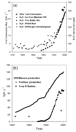
Figure 7.16. (a) Changes in the emissions of fuel combustion NOx and atmosphericN2Omixing ratios since 1750 . Mixing ratios ofN2Oprovide the atmospheric measurement constraint on global changes in the N cycle. (b) Changes in the indices of the global agricultural N cycle since 1850 : the production of manure, fertilizer and estimates of crop N fixation. For data sources see http://www-eosdis.ornl.gov/ ( Holland et al., 2005b [NPR, SRC] ) and http://www.cmdl.noaa.gov/. Figure adapted from Holland et al. 2005c [JoC, SRC] ).
Since the TAR, both top-down and bottom-up estimates ofN2Ohave been refined. Agriculture remains the single biggest anthropogenicN2Osource ( Bouwman et al., 2002 [JoC, MoS] ;( Smith and Conen, 2004; ) del Grosso et al., 2005 [MoS] ). Land use change continues to affectN2Oand NO emissions ( (Neill et al., 2005 ) ): logging is estimated to increaseN2Oand NO emissions by 30 to 350% depending on conditions ( (Keller et al., 2005 ) ). Both studies underscore the importance of N supply, temperature and moisture as regulators of trace gas emissions. The inclusion of several minor sources (human excreta, landfills and atmospheric deposition) has increased the total bottom-up budget to 20.6 TgN yr–1 ( Bouwman et al., 2002 [JoC, MoS] ). Sources ofN2Onow estimated since the TAR include coastalN2Ofluxes of 0.2 TgN yr–1 (±70%; Nevison et al., 2004 [JoC, ARC] ) and river and estuarineN2Ofluxes of 1.5 TgN yr–1 ( Kroeze et al., 2005 [MoS] ). Box model calculations show the additional river and estuarine sources to be consistent with the observed rise in atmosphericN2O(Kroeze et al., 2005 ).
Top-down estimates of surface sources use observed concentrations to constrain total sources and their spatial distributions. A simple calculation, using the present-dayN2Oburden divided by its atmospheric lifetime, yields a global stratospheric loss of about 12.5 ± 2.5 TgN yr–1.Combined with the atmospheric increase, this loss yields a surface source of 16 TgN yr–1.An inverse modelling study of the surface flux ofN2Oyields a global source of 17.2 to 17.4 TgN yr–1 with an estimated uncertainty of 1.4 (1 standard deviation; Hirsch et al., 2006 [JoC, MoS] ). The largest sources ofN2Oare from land at tropical latitudes, the majority located north of the equator. The Hirsch et al. inversion results further suggest thatN2Osource estimates from agriculture and fertilizer may have increased markedly over the last three decades when compared with an earlier inverse model estimate ( Prinn et al., 1990 [JoC, ARC] ). Bottom-up estimates, which sum individual source estimates, are more evenly distributed with latitude and lack temporal variability. However, there is clear consistency between top-down and bottom-up global source estimates, which are 17.3 (15.8–18.4) and 17.7 (8.5–27.7) TgN yr–1,respectively.
Concentrations of NOx and reduced nitrogen (NHx = NH3 + ammonium ion (NH4+)) are difficult to measure because the atmospheric lifetimes of hours to days instead of years generate pronounced spatial and temporal variations in their distributions. Atmospheric concentrations of NOx and NHx vary more regionally and temporally than concentrations ofN2O. Total global NOx emissions have increased from an estimated pre-industrial value of 12 TgN yr–1 ( Holland et al., 1999 [SRC] ; Galloway et al., 2004 [MoS] ) to between 42 and 47 TgN yr–1 in 2000 ( Table 7.7 Lamarque et al. 2005a [JoC] ) forecast them to be 105 to 131 TgN yr–1 by 2100 . The range of surface NOx emissions (excluding lightning and aircraft) used in the current generation of global models is 33 to 45 TgN yr–1 with small ranges for individual sources. The agreement reflects the use of similar inventories and parametrizations. Current estimates of NOx emissions from fossil fuel combustion are smaller than in the TAR.
Since the TAR, estimates of tropospheric NO2 columns from space by the Global Ozone Monitoring Experiment (GOME, launched in 1995 ) and the SCanning Imaging Absorption SpectroMeter for Atmospheric CHartographY (SCIAMACHY, launched in 2002 ( (Richter and Burrows, 2002; ) ( Heue et al., 2005 ) ) provide constraints on estimates of NOx emissions ( Leue et al., 2001 [JoC] Martin et al. 2003a [JoC] ) use GOME data to estimate a global surface source of NOx of 38 TgN yr–1 for 1996 to 1997 with an uncertainty factor of 1.6. ( Jaeglé et al. 2005 ) ) partition the surface NOx source inferred from GOME into 25.6 TgN yr–1 from fuels, 5.9 TgN yr–1 from biomass burning and 8.9 TgN yr–1 from soils. Interactions between soil emissions and scavenging by plant canopies have a significant impact on soil NOx emissions to the free troposphere: the impact may be greatest in subtropical and tropical regions where emissions from fuel combustion are rising ( Ganzeveld et al., 2002 [JoC] Boersma et al. 2005 [MoS] ) find that GOME data constrain the global lightning NOx source for 1997 to the range 1.1 to 6.4 TgN yr–1.Comparison of the tropospheric NO2 column of three state-of-the-art retrievals from GOME for the year 2000 with model results from 17 global atmospheric chemistry models highlights significant differences among the various models and among the three GOME retrievals( Figure 7.17 ,van Noije et al., 2006 [MoS, SRC] ). The discrepancies among the retrievals (10 to 50% in the annual mean over polluted regions) indicate that the previously estimated retrieval uncertainties have a large systematic component. Top-down estimates of NOx emissions from satellite retrievals of tropospheric NO2 are strongly dependent on the choice of model and retrieval.
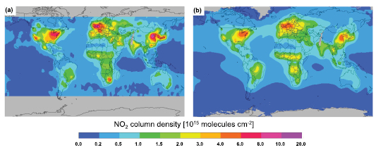
Figure 7.17. Tropospheric column NO2 from (a) satellite measurements and (b) atmospheric chemistry models. The maps represent ensemble average annual mean tropospheric NO2 column density maps for the year 2000 . The satellite retrieval ensemble comprises three state-of-the-art retrievals from GOME; the model ensemble includes 17 global atmospheric chemistry models. These maps were obtained after smoothing the data to a common horizontal resolution of 5° × 5° (adapted from van Noije et al., 2006 [MoS, SRC] ).
Knowledge of the spatial distribution of NOx emissions has evolved significantly since the TAR. An Asian increase in emissions has been compensated by a European decrease over the past decade ( Naja et al., 2003 [JoC] Richter et al. 2005 [JoC] ; see also Irie et al., 2005 [JoC] ) use trends for 1996 to 2004 observed by GOME and SCIAMACHY to deduce a 50% increase in NOx emissions over industrial areas of China. Observations of NO2 in shipping lanes from GOME ( Beirle et al., 2004 [JoC, MoS] ) and SCIAMACHY ( Richter et al., 2004 [NPR, JoC] ) give values at the low end of emission inventories. Data from GOME and SCIAMACHY further reveal large pulses of soil NOx emissions associated with rain ( Jaeglé et al., 2004 [JoC] ) and fertilizer application ( Bertram et al., 2005 [JoC] ).
All indices show an increase since pre-industrial times in the intensity of agricultural nitrogen cycling, the primary source of NH3 emissions( Figure 7.16 band Table 7.7 ;Bouwman et al., 2002 [JoC, MoS] ). Total global NH3 emissions have increased from an estimated pre-industrial value of 11 TgN yr–1 to 54 TgN yr–1 for 2000 ( Holland et al., 1999 [SRC] ; Galloway et al., 2004 [MoS] ), and are projected to increase to 116 TgN yr–1 by 2050 .
Table 7.7. Global sources (TgN yr–1)of NOx,NH3 andN2Ofor the 1990 s.
| Source | NOx | NH3 | N2O | |||
|---|---|---|---|---|---|---|
| TARa | AR4b | TARa | AR4a | TARc | AR4 | |
| Anthropogenic sources | ||||||
| Fossil fuel combustion & industrial processes | 33 (20–24) | 25.6 (21–28) | 0.3 (0.1–0.5) | 2.5d | 1.3/0.7 (0.2–1.8) | 0.7 (0.2–1.8)d |
| Aircraft | 0.7 (0.2–0.9) | – e (0.5–0.8) | - | - | - | - |
| Agriculture | 2.3f (0–4) | 1.6g | 34.2 (16–48) | 35g (16–48) | 6.3/2.9 (0.9–17.9) | 2.8 (1.7–4.8)g |
| Biomass and biofuel burning | 7.1 (2–12) | 5.9 (6–12) | 5.7 (3–8) | 5.4d (3–8) | 0.5 (0.2–1.0) | 0.7 (0.2–1.0)g |
| Human excreta | – | – | 2.6 (1.3–3.9) | 2.6g (1.3–3.9) | – | 0.2g (0.1–0.3)h |
| Rivers, estuaries, coastal zones | – | – | – | – | – | 1.7 (0.5–2.9)i |
| Atmospheric deposition | – | 0.3g | – | – | – | 0.6j (0.3–0.9)h |
| Anthropogenic total | 43.1 | 33.4 | 42.8 | 45.5 | 8.1/4.1 | 6.7 |
| Natural sources | ||||||
| Soils under natural vegetation | 3.3f (3–8) | 7.3j (5–8) | 2.4 (1–10) | 2.4g (1–10) | 6.0/6.6 (3.3–9.9) | 6.6 (3.3–9.0)g |
| Oceans | – | – | 8.2 (3–16) | 8.2g (3–6) | 3.0/3.6 (1.0–5.7) | 3.8 (1.8–5.8)k |
| Lightning | 5(2–12) | 1.1–6.4 (3–7) | – | – | – | – |
| Atmospheric chemistry | <0.5 | – | – | – | 0.6 (0.3–1.2) | 0.6 (0.3–1.2)c |
| Natural total | 8.8 | 8.4–13.7 | 10.6 | 10.6 | 9.6/10.8 | 11.0 |
| Total sources | 51.9 (27.2–60.9) | 41.8–47.1 (37.4–57.7) | 53.4 (40–70) | 56.1 (26.8–78.4) | 17.7/14.9 (5.9–37.5) | 17.7 (8.5–27.7) |
The primary sink for NHx and NOx and their reaction products is wet and dry deposition. Estimates of the removal rates of both NHx and NOx are provided by measurements of wet deposition over the USA and Western Europe to quantify acid rain inputs ( Hauglustaine et al., 2004 [JoC, MoS, SRC] ; Holland et al., 2005a [MoS, SRC] ; Lamarque et al., 2005a [JoC] ). Chemical transport models represent the wet and dry deposition of NOx and NHx and their reaction products. A study of 29 simulations with 6 different tropospheric chemistry models, focusing on present-day and 2100 conditions for NOx and its reaction products, projects an average increase in N deposition over land by a factor of 2.5 by 2100 ( Lamarque et al., 2005b [JoC, MoS] ), mostly due to increases in NOx emissions. Nitrogen deposition rates over Asia are projected to increase by a factor of 1.4 to 2 by 2030 . Climate contributions to the changes in oxidized N deposition are limited by the models’ ability to represent changes in precipitation patterns. An intercomparison of 26 global atmospheric chemistry models demonstrates that current scenarios and projections are not sufficient to stabilise or reduce N deposition or ozone pollution before 2030 ( Dentener et al., 2006 [SRC] ).
7.4.3. Molecular Hydrogen
Increased interest in atmosphericH2 is due to its potential role as an indirect greenhouse gas ( Derwent et al., 2001 [JoC, SRC] ) and expected perturbations of its budget in a prospective ‘hydrogen economy’ ( Schultz et al., 2003 [JoC, MoS, SRC] ; Tromp et al., 2003 [JoC] ; Warwick et al., 2004 [JoC, MoS] ). Potential consequences of increasedH2 emissions include a reduction of global oxidizing capacity (presentlyH2 constitutes 5 to 10% of the global average OH sink, Schultz et al., 2003 [JoC, MoS, SRC] ) and increased formation of water vapour, which could lead to increased cirrus formation in the troposphere and increased polar stratospheric clouds (PSCs) and additional cooling in the stratosphere, thereby leading to more efficient ozone depletion ( Tromp et al., 2003 [JoC] ).
Studies of the global troposphericH2 budget (see Table 7.8 )generally agree on a total source strength of between 70 and 90 Tg(H2) yr–1,which is approximately balanced by its sinks. About half of theH2 is produced in the atmosphere via photolysis of formaldehyde (CH2O), which itself originates from the oxidation of CH4 and other volatile organic compounds. The other half stems mostly from the combustion of fossil fuels (e.g., car exhaust) and biomass burning. About 10% of the globalH2 source is due to ocean biochemistry and N fixation in soils. Presently, about 50 Tg(H2)yr–1 are produced in the industrial sector, mostly for the petrochemical industry (e.g., refineries) ( Lovins, 2003 [NPR] ). Evaporative losses of industrialH2 are generally assumed to be negligible ( Zittel and Altmann, 1996 [NPR] ). The dominant sink of atmosphericH2 is deposition with catalytic destruction by soil microorganisms and possibly enzymes ( (Conrad and Seiler, 1981 ) ). The seasonal cycle of observedH2 concentrations implies an atmospheric lifetime of about 2 years ( Novelli et al., 1999 [JoC] ; Simmonds et al., 2000 [JoC] ; Hauglustaine and Ehhalt, 2002 [JoC, MoS, SRC] ), whereas the lifetime with respect to OH oxidation is 9 to 10 years, which implies that the deposition sink is about three to four times as large as the oxidation. Loss ofH2 to the stratosphere and its subsequent escape to space is negligible for the troposphericH2 budget, because the budgets of the troposphere and stratosphere are largely decoupled ( Warneck, 1988 [NPR] ).
Table 7.8. Summary of global budget studies of atmosphericH2 (Tg(H2)yr–1).
| Sanderson et al. (2003a) | Hauglustaine and Ehhalt (2002) | Novelli et al. (1999) | Ehhalt (1999) | Warneck (1988) | Seiler and Conrad (1987) | |
|---|---|---|---|---|---|---|
| Sources | ||||||
| Oxidation of CH4 and VOC | 30.2 | 31 | 40 ± 16 | 35 ± 15 | 50 | 40 ± 15 |
| Fossil fuel combustion | 20 | 16 | 15 ± 10 | 15 ± 10 | 17 | 20 ± 10 |
| Biomass burning | 20 | 13 | 16 ± 11 | 16 ± 5 | 15 | 20 ± 10 |
| N2 fixation | 4 | 5 | 3 ± 1 | 3 ± 2 | 3 | 3± 2 |
| Ocean release | 4 | 5 | 3 ± 2 | 3 ± 2 | 4 | 4± 2 |
| Volcanoes | – | – | – | – | 0.2 | – |
| Total | 78.2 | 70 | 77 ± 16 | 71 ± 20 | 89 | 87 |
| Sinks | ||||||
| Deposition | 58.3 | 55 | 56 ± 41 | 40 ± 30 | 78 | 90 ± 20 |
| Oxidation by OH | 17.1 | 15 | 19 ± 5 | 25 ± 5 | 11 | 8± 3 |
| Total | 74.4 | 70 | 75 ± 41 | 65 ± 30 | 89 | 98 |
Estimates ofH2 required to fuel a future carbon-free energy system are highly uncertain and depend on the technology as well as the fraction of energy that might be provided byH2.In the future,H2 emissions could at most double: the impact on global oxidizing capacity and stratospheric temperatures and ozone concentrations is estimated to be small ( Schultz et al., 2003 [JoC, MoS, SRC] ; Warwick et al., 2004 [JoC, MoS] ). According to Schultz et al. 2003 [JoC, MoS, SRC] ), the side effects of a globalH2 economy could have a stronger impact on global climate and air pollution. Global oxidizing capacity is predominantly controlled by the concentration of NOx.Large-scale introduction ofH2-powered vehicles would lead to a significant decrease in global NOx emissions, leading to a reduction in OH of the order of 5 to 10%. Reduced NOx levels could also significantly reduce tropospheric ozone concentrations in urban areas. Despite the expected large-scale use of natural gas forH2 production, the impact of aH2 economy on the global CH4 budget is likely to be small, except for the feedback between reduced oxidizing capacity (via NOx reduction) and CH4 lifetime.
7.4.4 Global Tropospheric Ozone
7.4.4.1 Present-Day Budgets of Ozone and its Precursors
Tropospheric ozone is (after CO2 and CH4)the third most important contributor to greenhouse radiative forcing. Trends over the 20th century are discussed in Chapter2 .Ozone is produced in the troposphere by photochemical oxidation of CO, CH4 and non-methane VOCs (NMVOCs) in the presence of NOx.Stratosphere-troposphere exchange (STE) is another source of ozone to the troposphere. Loss of tropospheric ozone takes place through chemical reactions and dry deposition. Understanding of tropospheric ozone and its relationship to sources requires three-dimensional tropospheric chemistry models that describe the complex nonlinear chemistry involved and its coupling to transport.
The past decade has seen considerable development in global models of tropospheric ozone, and the current generation of models can reproduce most climatological features of ozone observations. The TAR reported global tropospheric ozone budgets from 11 models in the 1996 to 2000 literature. Table 7.9 presents an update to the post- 2000 literature, including a recent intercomparison of 25 models ( Stevenson et al., 2006 [JoC, MoS, SRC] ). Models concur that chemical production and loss are the principal terms in the global budget. Although STE is only a minor term in the global budget, it delivers ozone to the upper troposphere where its lifetime is particularly long (about one month, limited by transport to the lower troposphere) and where it is of most importance from a radiative forcing perspective.
The post- 2000 model budgets in Table 7.9 show major differences relative to the older generation TAR models: on average a 34% weaker STE, a 35% stronger chemical production, a 10% larger tropospheric ozone burden, a 16% higher deposition velocity and a 10% shorter chemical lifetime. It is now well established that many of the older studies overestimated STE, as observational constraints in the lower stratosphere impose an STE ozone flux of 540 ± 140 Tg yr–1 ( Gettelman et al., 1997 [JoC, ARC] ; Olsen et al., 2001 [JoC, ARC] ). Overestimation of the STE flux appears to be most serious in models using assimilated meteorological data, due to the effect of assimilation on vertical motions ( Douglass et al., 2003 [JoC, MoS] ; Schoeberl et al., 2003 [JoC, MoS] ; Tan et al., 2004 [JoC, ARC] ; van Noije et al., 2004 [JoC, MoS, SRC] ). The newer models correct for this effect by using dynamic flux boundary conditions in the tropopause region ( McLinden et al., 2000 [JoC, MoS] ) or by relaxing model results to observed climatology ( Horowitz et al., 2003 [JoC, MoS] ). Such corrections, although matching the global STE flux constraints, may still induce errors in the location of the transport ( Hudman et al., 2004 [JoC] ) with implications for the degree of stratospheric influence on tropospheric concentrations ( Fusco and Logan, 2003 [JoC, MoS] ).
Table 7.9. Global budgets of tropospheric ozone (Tg yr–1)for the present-day atmospherea.
| Reference | Modelb | Stratosphere-Troposphere Exchange | Chemical Productionc | Chemical Lossc | Dry Deposition | Burden (Tg) | Lifetimed (days) |
|---|---|---|---|---|---|---|---|
| TARe | 11 models | 770 ± 400 | 3420 ± 770 | 3470 ± 520 | 770 ± 180 | 300 ± 30 | 24 ± 2 |
| Lelieveld and Dentener (2000) | TM3 | 570 | 3310 | 3170 | 710 | 350 | 33 |
| Bey et al. (2001) | GEOS-Chem | 470 | 4900 | 4300 | 1070 | 320 | 22 |
| Sudo et al. (2002b) | CHASER | 593 | 4895 | 4498 | 990 | 322 | 25 |
| Horowitz et al. (2003) | MOZART-2 | 340 | 5260 | 4750 | 860 | 360 | 23 |
| Von Kuhlmann et al. (2003) | MATCH-MPIC | 540 | 4560 | 4290 | 820 | 290 | 21 |
| Shindell et al. (2003) | GISS | 417 | NRf | NR | 1470 | 349 | NR |
| Hauglustaine et al. (2004) | LMDz-INCA | 523 | 4486 | 3918 | 1090 | 296 | 28 |
| Park et al. (2004) | UMD-CTM | 480 | NR | NR | 1290 | 340 | NR |
| Rotman et al. (2004) | IMPACT | 660 | NR | NR | 830 | NR | NR |
| Wong et al. (2004) | SUNY/UiO GCCM | 600 | NR | NR | 1100 | 376 | NR |
| Stevenson et al. (2004) | STOCHEM | 395 | 4980 | 4420 | 950 | 273 | 19 |
| Wild et al. (2004) | FRSGC/UCI | 520 | 4090 | 3850 | 760 | 283 | 22 |
| Folberth et al. (2006) | LMDz-INCA | 715 | 4436 | 3890 | 1261 | 303 | 28 |
| Stevenson et al. (2006) | 25 models | 520 ± 200 | 5060 ± 570 | 4560 ± 720 | 1010 ± 220 | 340 ± 40 | 22 ± 2 |
The faster chemical production and loss of ozone in the current generation of models could reflect improved treatment of NMVOC sources and chemistry ( Houweling et al., 1998 [JoC, SRC] ), ultraviolet (UV) actinic fluxes ( Bey et al., 2001 [JoC, MoS] ) and deep convection ( Horowitz et al., 2003 [JoC, MoS] ), as well as higher NOx emissions ( Stevenson et al., 2006 [JoC, MoS, SRC] ). Subtracting ozone chemical production and loss terms in Table 7.9 indicates that the current generation of models has net production of ozone in the troposphere, while the TAR models had net loss, reflecting the decrease in STE. Net production is not a useful quantity in analysing the ozone budget because (1) it represents only a small residual between production and loss and (2) it reflects a balance between STE and dry deposition, both of which are usually parametrized in models.
Detailed budgets of ozone precursors were presented in the TAR. The most important precursors are CH4 and NOx ( Wang et al., 1998 [JoC, MoS, SRC] ;( Grenfell et al., 2003; ) Dentener et al., 2005 [MoS, SRC] ). Methane is in general not simulated explicitly in ozone models and is instead constrained from observations. Nitrogen oxides are explicitly simulated and proper representation of sources and chemistry is critical for the ozone simulation. The lightning source is particularly uncertain ( Nesbitt et al., 2000 [JoC, MoS] ; Tie et al., 2002 [SRC] ), yet is of great importance because of the high production efficiency of ozone in the tropical upper troposphere. The range of the global lightning NOx source presently used in models (3–7 TgN yr–1)is adjusted to match atmospheric observations of ozone and NOx,although large model uncertainties in deep convection and lightning vertical distributions detract from the strength of this constraint. Process-based models tend to predict higher lightning emissions (5–20 TgN yr–1 ;Price et al., 1997 [JoC, ARC] ).
Other significant precursors for tropospheric ozone are CO and NMVOCs, the most important of which is biogenic isoprene. Satellite measurements of CO from the Measurements of Pollution in the Troposphere (MOPITT) instrument launched in 1999 ( Edwards et al., 2004 [JoC] ) have provided important new constraints for CO emissions, pointing in particular to an underestimate of Asian sources in current inventories ( Kasibhatla et al., 2002 [JoC, MoS] ; Arellano et al., 2004 [JoC, MoS] ; Heald et al., 2004 [JoC, MoS] ; Petron et al., 2004 [JoC] ), as confirmed also by aircraft observations of Asian outflow ( Palmer et al., 2003a [JoC] ; Allen et al., 2004 [JoC, MoS] ). Satellite measurements of formaldehyde columns from the GOME instrument ( Chance et al., 2000 [JoC] ) have been used to place independent constraints on isoprene emissions and indicate values generally consistent with current inventories, although with significant regional discrepancies ( Palmer et al., 2003b [JoC] ; Shim et al., 2005 [JoC] ).
Afew recent studies have examined the effect of aerosols on global tropospheric ozone involving both heterogeneous chemistry and perturbations to actinic fluxes. Jacob 2000 [SRC] ) reviewed the heterogeneous chemistry involved. Hydrolysis of dinitrogen pentoxide (N2O5)in aerosols is a well-known sink for NOx,but other processes involving reactive uptake of the hydroperoxyl radical (HO2), NO2 and ozone itself could also be significant. Martin et al. 2003b [JoC] ) find that including these processes along with effects of aerosols on UV radiation in a global Chemical Transport Model (CTM) reduced ozone production rates by 6% globally, with larger effects over aerosol source regions.
Although the current generation of tropospheric ozone models is generally successful in describing the principal features of the present-day global ozone distribution, there is much less confidence in the ability to reproduce the changes in ozone associated with perturbations of emissions or climate. There are major discrepancies with observed long-term trends in ozone concentrations over the 20th century ( Hauglustaine and Brasseur, 2001 [JoC, MoS, SRC] ; Mickley et al., 2001 [JoC, MoS, SRC] ; Shindell and Favulegi, 2002; Shindell et al., 2003 [MoS] ; Lamarque et al., 2005c [JoC] ), including after 1970 when the reliability of observed ozone trends is high ( Fusco and Logan, 2003 [JoC, MoS] ). Resolving these discrepancies is needed to establish confidence in the models.
7.4.4.2 Effects of Climate Change
Climate change can affect tropospheric ozone by modifying emissions of precursors, chemistry, transport and removal (European Commission, 2003 ). These and other effects are discussed below. They could represent positive or negative feedbacks to climate change.
7.4.4.2.1 Effects on emissions
Climate change affects the sources of ozone precursors through physical response (lightning), biological response (soils, vegetation, biomass burning) and human response (energy generation, land use, agriculture). It is generally expected that lightning will increase in a warmer climate ( Price and Rind, 1994a [JoC, ARC] ; Brasseur et al., 2005 [JoC, MoS, SRC] ; Hauglustaine et al., 2005 [JoC, MoS, SRC] ), although a GCM study by Stevenson et al. 2006 [JoC, MoS, SRC] ) for the 2030 climate finds no global increase but instead a shift from the tropics to mid-latitudes. Perturbations to lightning could have a large effect on ozone in the upper troposphere ( Toumi et al., 1996 [JoC, ARC] ; Thompson et al., 2000 [JoC] ; Martin et al., 2002 [JoC, MoS] ; Wong et al., 2004 [JoC, MoS] Mickley et al. 2001 [JoC, MoS, SRC] ) find that observed long-term trends in ozone over the past century might be explainable by an increase in lightning.
Biomass burning in the tropics and at high latitudes is likely to increase with climate change, both as a result of increased lightning and as a result of increasing temperatures and dryness ( Price and Rind, 1994b [JoC, ARC] ; Stocks et al., 1998 [JoC] ; A. Williams et al., 2001 [JoC] ; Brown et al., 2004 [JoC] ). Biomass burning is known to make a large contribution to the budget of ozone in the tropical troposphere ( Thompson et al., 1996 [JoC] ), and there is evidence that boreal forest fires can enhance ozone throughout the extratropical NH ( Jaffe et al., 2004 [JoC] ). With climate warming, it is likely that boreal fires will increase due to a shorter duration of the seasonal snowpack and decreased soil moisture ( (Kasischke et al., 1995 ) ).
Biogenic VOC emissions may be highly sensitive to climate change. The most important global ozone precursors are CH4 and isoprene. The effect of climate change on CH4 is discussed in Section 7.4.1 .The effect on NMVOCs was examined by Constable et al. 1999 [MoS, SRC] Sanderson et al. 2003b [JoC] and Lathière et al. 2005 [JoC, MoS] ). Although biogenic NMVOC emissions increase with increasing temperature, all three studies concur that climate-driven changes in vegetation types unfavourable to isoprene emissions (notably the recession of tropical forests) would partly compensate for the effect of warming in terms of ozone generation.
7.4.4.2.2 Effects on chemistry
Changes in temperature, humidity and UV radiation intensity brought about by climate change could affect ozone significantly. Simulations with GCMs by Stevenson et al. 2000 [JoC, MoS, SRC] and Grewe et al. 2001 [JoC, MoS] ) for the 21st century indicate a decrease in the lifetime of tropospheric ozone as increasing water vapour enhances the dominant ozone sink from the oxygen radical in the 1D excited state (O(1D)) plus water (H2O) reaction. Stevenson et al. 2006 [JoC, MoS, SRC] ) find similar results in an intercomparison of nine models for 2030 compared with 2000 climate. However, regional ozone pollution may increase in the future climate as a result of higher temperatures (see Section 7.6 , Box 7.4 ).
7.4.4.2.3 Effects on transport
Changes in atmospheric circulation could have a major effect on tropospheric ozone. Studies using GCMs concur that STE should increase in the future climate because of the stronger Brewer-Dobson stratospheric circulation ( Sudo et al., 2002a [JoC, MoS, ARC] ; Collins et al., 2003 [JoC, MoS] ; Zeng and Pyle, 2003 [JoC, MoS] ; Hauglustaine et al., 2005 [JoC, MoS, SRC] ; Stevenson et al., 2005 [NPR, SRC] ). Changes in vertical transport within the troposphere are also important, in view of the rapid increase in both ozone production efficiency and ozone lifetime with altitude. Convection is expected to intensify as climate warms ( Rind et al., 2001 [JoC, ARC] ), although this might not be the case in the tropics ( Stevenson et al., 2005 [NPR, SRC] ). The implications are complex, as recently discussed by Pickering et al. 2001 [JoC] Lawrence et al. 2003 [JoC] Olivié et al. 2004 [JoC, MoS] Doherty et al. 2005 [MoS, SRC] and Li et al. 2005 [JoC] ). On the one hand, convection brings down ozone-rich air from the upper troposphere to the lower troposphere where it is rapidly destroyed, and replaces it with low-ozone air. On the other hand, injection of NOx to the upper troposphere greatly increases its ozone production efficiency.
7.4.5 The Hydroxyl Radical
The hydroxyl radical (OH) is the primary cleansing agent of the lower atmosphere, providing the dominant sink for many greenhouse gases (e.g., CH4,hydrochlorofluorocarbons (HCFCs), hydrofluorocarbons) and pollutants (e.g., CO, non-methane hydrocarbons). Steady-state lifetimes of these trace gases are determined by the morphology of their atmospheric distribution, the kinetics of their reaction with OH and the OH distribution. Local abundance of OH is controlled mainly by local abundances of NOx,CO, CH4 and higher hydrocarbons, ozone, water vapour, as well as the intensity of solar UV radiation at wavelengths shorter than 0.310 µm. New laboratory and field work also shows significant formation of O(1D) from ozone photolysis in the wavelength range between 0.310 µm and 0.350 µm ( Matsumi et al., 2002 [JoC] ; Hofzumahaus et al., 2004 [JoC, MoS] ). The primary source of tropospheric OH is a pair of reactions starting with the photodissociation of ozone by solar UV radiation.
Additionally, in the remote, and in particular upper, troposphere, photodissociation of oxygenated volatile organic chemicals such as peroxides, acetone and other ketones, alcohols, and aldehydes may be the dominant sources of OH radical (e.g., Müller and Brasseur, 1999 [JoC, SRC] ; Collins et al., 1999 [JoC, SRC] ; Jaeglé et al., 2001 [SRC] ; Tie et al., 2003 [JoC, SRC] ; Singh et al., 2004 [JoC] ). Over continents, measurements in the lower troposphere suggest that processing of unsaturated hydrocarbons or photolysis of carbonyls can also sustain a large pool of radicals (e.g., ( Handisides et al., 2003; ) Heard et al., 2004 [JoC] ). Furthermore, the net formation of OH by photolysis of nitrous acid (HONO) was found to be the dominant OH radical source in urban atmospheres (e.g., ( Ren et al., 2003 ) ) and in a forest canopy ( Kleffmann et al., 2005 [JoC] ). The hydroxyl radical reacts with many atmospheric trace gases, in most cases as the first and rate-determining step of a reaction chain that leads to more or less complete oxidation of the compound. These chains often lead to formation of HO2,which then reacts with ozone or NO to recycle back to OH. Tropospheric OH and HO2 are lost through radical-radical reactions leading to the formation of peroxides or with NO2 to form nitric acid (HNO3). Sources and sinks of OH involve most of the fast photochemistry of the troposphere.
7.4.5.1 Changes in the Hydroxyl Radical Over Time
7.4.5.1.1 Impact of emissions
Because of its dependence on CH4 and other pollutants, tropospheric OH is also expected to have changed since the pre-industrial era and to change in the future. Pre-industrial OH is likely to have been different than today, but because of the counteracting effects of higher CO and CH4 (decreasing OH) and increased NOx and ozone (increasing OH) there is still little consensus on the magnitude of this change. Several model studies suggest a decline in weighted global mean OH from pre-industrial time to the present of less than 10% ( Shindell et al., 2001 [JoC, MoS] ; Lelieveld et al., 2002a [JoC, SRC] ; Lamarque et al., 2005a [JoC] ). Other studies have reported larger decreases in global OH of 16% ( Mickley et al., 1999 [JoC, MoS] ), 25% ( Wong et al., 2004 [JoC, MoS] ) and 33% ( Hauglustaine and Brasseur, 2001 [JoC, MoS, SRC] ). The model study by Lelieveld et al. 2002b [JoC] ) suggests that during the past century, OH concentration decreased substantially in the marine troposphere through reaction with CH4 and CO. However, on a global scale it has been compensated by an increase over the continents associated with strong emissions of NOx.
Karlsdottir and Isaksen 2000 [JoC] ) used a three-dimensional CTM accounting for varying NOx,CO and NMVOC emissions and found a positive trend in OH of 0.43% yr–1 over the period 1980 to 1996 Dentener et al. 2003a [JoC, SRC] ,b), with a three-dimensional CTM accounting for varying emissions of ozone precursors and CH4,meteorology and column ozone, derive a positive trend of 0.26% yr–1 over the 1979 to 1993 period. J. Wang et al. 2004 [Ambiguous] ) also use a three-dimensional CTM accounting for interannual variations in CH4 and CO emissions, transport and column ozone to analyse the trend in CH4 from 1988 to 1997 . They do not account for interannual variability of a number of other variables that affect OH such as concentrations of NOx,tropospheric ozone and NMVOCs. They also derive a positive trend in OH over the period considered of 0.63% yr–1.Their calculated trend in OH is associated primarily with the negative trend in the overhead column ozone over the period considered and the trend is reduced to 0.16% yr–1 when the total ozone column is held constant.
Future changes in OH depend on relative changes in hydrocarbons compared with NOx abundances. In the TAR, Prather et al. 2001 [NPR, ARC] ), using scenarios reported in the IPCC SRES ( IPCC, 2000 [NPR] ) and on the basis of a comparison of results from 14 models, predicted that global OH could decrease by 10 to 18% by 2100 for five emission scenarios and increase by 5% for one scenario (which assumes large decreases in CH4 and other ozone precursor emissions). Based on a different emission scenario for future emissions, Wang and Prinn 1999 [MoS, ARC] ) also predicted an OH decrease of 16 ± 3% in 2100 .
7.4.5.1.2 Effects of climate change
In addition to the emission changes, future increases in greenhouse gases could also induce changes in OH, arising through direct participation in OH-controlling chemistry and indirectly through stratospheric ozone changes that could increase solar UV radiation in the troposphere. OH will also be affected by changes in temperature, humidity and clouds or climate change effects on biogenic emissions of CH4 and other ozone precursors. Changes in tropospheric water could have important chemical repercussions. The reaction between water vapour and electronically excited oxygen atoms constitutes the major source of tropospheric OH. So, in a warmer climate characterised by increased specific humidity, the abundance of OH is expected to increase. This effect was proposed by Pinto and Khalil 1991 [JoC] ) to explain the variation of OH during the cold dry Last Glacial Maximum (LGM). It was quantified by Martinerie et al. 1995 [JoC, MoS, SRC] ) who calculated that the global mean OH concentration during the LGM was 7% lower than at present because the atmospheric water vapour concentration was lower during that period. Valdes et al. 2005 [NPR, JoC] ) estimate that the cold and dry LGM climate was responsible for a 7% decrease in global OH. Brasseur et al. 1998 [JoC, MoS, SRC] and Johnson et al. 1999 [JoC, MoS, SRC] ) estimated that in a warmer (doubled atmospheric CO2)climate, the global and annual mean OH concentration would increase by 7% and 12.5%, respectively. More recently, Hauglustaine et al. 2005 [JoC, MoS, SRC] ) use a climate-chemistry three-dimensional model to estimate a 16% reduction in global OH from the present day to 2100 accounting solely for changes in surface emissions. The effect of climate change and mainly of increased water vapour in this model is to increase global OH by 13%. In this study, the competing effects of emissions and climate change maintain the future global average OH concentration close to its present-day value. The importance of the water vapour distribution to global OH is illustrated by Lamarque et al. 2005a [JoC] ), who show that under reduced aerosol emissions, a warmer and moister climate significantly increases global OH concentration.
Changes in lightning NOx emissions in a warmer climate may also affect OH. Labrador et al. 2004 [JoC] ) show that global OH is sensitive to the magnitude of lightning NOx emissions, and increases by 10% and 23% when global lightning is increased by a factor of 2 and 4, respectively, from a 5 TgN yr–1 best estimate. Similar sensitivity of global OH to the lightning source was estimated by Wang et al. 1998 [JoC, MoS, SRC] ), who calculated a 10.6% increase in OH for a doubling of the source (from 3 to 6 TgN yr–1). Regarding the large uncertainty about lightning emissions and the sensitivity of OH to the total amount of N emitted, an improved understanding of this source appears important for the ability to simulate OH accurately over time.
7.4.5.2 Consequences for Lifetimes
7.4.5.2.1 Lifetime definition
The global instantaneous atmospheric lifetime of a trace gas in the atmosphere is obtained by integrating the loss frequency l over the atmospheric domain considered. The integral must be weighted by the distribution of the trace gas on which the sink processes act. Considering a distribution of the trace gas C(x,y,z,t), a global instantaneous lifetime derived from the budget can be defined as:
where dv is an atmospheric volume element. This expression can be averaged over one year to determine the global and annual mean lifetime. The global atmospheric lifetime (also called ‘burden lifetime’ or ‘turnover lifetime’) characterises the time required to turn over the global atmospheric burden.
The global atmospheric lifetime characterises the time to achieve an e-fold decrease of the global atmospheric burden. Unfortunately τglobal is a constant only in very limited circumstances. In the case where the loss rate depends on the burden, the perturbation or pulse decay lifetime (τpert)is introduced (see Velders et al., 2005 [NPR] ). The perturbation lifetime is used to determine how a one-time pulse emission may decay as a function of time as needed for the calculation of Global Warming Potentials (GWPs). The perturbation lifetime can be distinctly different from the global atmospheric lifetime. For example, if the CH4 abundance increases above its present-day value due to a one-time emission, the time it takes for CH4 to decay back to its background value is longer than its global unperturbed atmospheric lifetime. This delay occurs because the added CH4 will cause a suppression of OH, in turn increasing the background CH4.Such feedbacks cause the decay time of a perturbation (τpert)to differ from the global atmospheric lifetime (τglobal). In the limit of small perturbations, the relation between the perturbation lifetime of a gas and its global atmospheric lifetime can be derived from a simple budget relationship as τpert = τglobal / (1– f), where the sensitivity coefficient f = dln(τglobal)/ dln(B). Prather et al. 2001 [NPR, ARC] ) estimated the feedback of CH4 to tropospheric OH and its lifetime and determined a sensitivity coefficient f = 0.28, giving a ratio τpert / τglobal of 1.4. Stevenson et al. 2006 [JoC, MoS, SRC] ), from 25 CTMs, calculate an ensemble mean and 1 standard deviation uncertainty in present-day CH4 global lifetime τglobal of 8.7 ± 1.3 years, which is the AR4 updated value. The corresponding perturbation lifetime that should be used in the GWP calculation is 12 ± 1.8 years.
Perturbation lifetimes can be estimated from global models by simulating the injection of a pulse of gas and tracking the decay of the added amount. The pulse of added CO, HCFCs or hydrocarbons, by causing the concentration of OH to decrease and thus the lifetime of CH4 to increase temporarily, causes a buildup of CH4 while the added burden of the gas persists. Thus, changes in the emissions of short-lived gases can generate long-lived perturbations as shown in global models ( Derwent et al., 2001 [JoC, SRC] ; Wild et al., 2001 [JoC, SRC] ; Collins et al., 2002 [JoC, SRC] ). Changes in tropospheric ozone accompany the CH4 decay on a 12-year time scale as an inherent component of this mode, a key example of chemical coupling in the troposphere. Any chemically reactive gas, whether a greenhouse gas or not, will produce some level of indirect greenhouse effect through its impact on atmospheric chemistry.
7.4.5.2.2 Changes in lifetime
Since OH is the primary oxidant in the atmosphere of many greenhouse gases including CH4 and hydrogenated halogen species, changes in OH will directly affect their lifetime in the atmosphere and hence their impact on the climate system. Recent studies show that interannual variations in the chemical removal of CH4 by OH have an important impact on the variability of the CH4 growth rate ( Johnson et al., 2002 [JoC, MoS, SRC] ; Warwick et al., 2002 [JoC] ; J. Wang et al., 2004 [Ambiguous] ). Variations in CH4 oxidation by OH contribute to a significant fraction of the observed variations in the annual accumulation rate of CH4 in the atmosphere. In particular, the 1992 to 1993 anomaly in the CH4 growth rate can be explained by fluctuations in OH and wetland emissions after the eruption of Mt. Pinatubo (J. Wang et al., 2004 [Ambiguous] ). CH4 variability simulated by Johnson et al. 2002 [JoC, MoS, SRC] ), resulting only from OH sink processes, also indicates that the ENSO cycle is the largest component of that variability. These findings are consistent with the variability of global OH reconstructed by Prinn et al. 2005 [JoC, ARC] Manning and Keeling 2006 [JoC, ARC] and Bousquet et al. 2005 [SRC] ), which is strongly affected by large-scale wildfires as in 1997 to 1998, by El Niño events and by the Mt. Pinatubo eruption.
The effect of climate change on tropospheric chemistry has been investigated in several studies. In most cases, the future CH4 lifetime increases when emissions increase and climate change is ignored ( Brasseur et al., 1998 [JoC, MoS, SRC] ; Stevenson et al., 2000 [JoC, MoS, SRC] ; Hauglustaine and Brasseur, 2001 [JoC, MoS, SRC] ; Prather et al., 2001 [NPR, ARC] ; Hauglustaine et al., 2005 [JoC, MoS, SRC] ). This reflects the fact that increased levels of CH4 and CO depress OH, reducing the CH4 sink. However, climate warming increases the temperature-dependent CH4 oxidation rate coefficient ( Johnson et al., 1999 [JoC, MoS, SRC] ), and increases in water vapour and NOx concentrations tend to increase OH. In most cases, these effects partly offset or exceed the CH4 lifetime increase due to emissions. As a consequence, the future CH4 lifetime calculated by Brasseur et al. 1998 [JoC, MoS, SRC] Stevenson et al. 2000 [JoC, MoS, SRC] and Hauglustaine et al. 2005 [JoC, MoS, SRC] ) remains relatively constant (within a few percent) over the 21st century. In their transient simulation over the period 1990 to 2100, Johnson et al. 2001 [JoC, MoS, SRC] ) find a dominant effect of climate change on OH in the free troposphere so that the global CH4 lifetime declines from about 9 years in 1990 to about 8.3 years by 2025 but does not change significantly thereafter. Hence the evolution of the CH4 lifetime depends on the relative timing of NOx and hydrocarbon emission changes in the emission scenarios, causing the calculated CH4 increase in 2100 to be reduced by 27% when climate change is considered. Stevenson et al. 2006 [JoC, MoS, SRC] ) reach a similar conclusion about the relatively constant CH4 lifetime. As a result of future changes in emissions, the CH4 steady-state lifetime simulated by 25 state-of-the-art CTMs increases by 2.7 ± 2.3% in 2030 from an ensemble mean of 8.7 ± 1.3 years for the present day (mean ± 1 standard deviation) for a current legislation scenario of future emissions of ozone precursors. Under the 2030 warmer climate scenario, the lifetime is reduced by 4.0 ± 1.8%: the total effect of both emission and climate changes reduces the CH4 lifetime by only 1.3%.
7.4.6 Stratospheric Ozone and Climate
From about 1980 to the mid- 1990 s a negative trend in globally averaged total ozone occurred, due primarily to an increase in Cl and bromine loading ( Montzka et al., 1999 [JoC, MoS, ARC] ). A reduction in halogen loading appears to have occurred recently ( Montzka et al., 2003 [JoC, ARC] ) as well as the beginning of ozone recovery (e.g., Newchurch et al., 2003 [JoC] ; Huck et al., 2005 [JoC, ARC] ; Reinsel et al., 2005 [JoC] ; Yang et al., 2005 [JoC] ). Evidence suggests that a sustainable recovery of ozone is not expected before the end of the current decade (e.g., Steinbrecht et al., 2004 [JoC] ; Dameris et al., 2006 [JoC, SRC] ). Atmospheric concentrations of LLGHGs have increased (see Chapter2 )and are expected to continue to increase, with consequences for the ozone layer. This section assesses current understanding of interactions and feedbacks between stratospheric ozone and climate. More detailed discussions can be found in recent reports (European Commission, 2003; IPCC/TEAP, 2005 ).
7.4.6.1 Interactions
Stratospheric ozone is affected by climate change through changes in dynamics and in the chemical composition of the troposphere and stratosphere. An increase in the concentrations of LLGHGs, especially CO2,cools the stratosphere, allowing the possibility of more PSCs, and alters the ozone distribution ( Rosenlof et al., 2001 [JoC, ARC] ; Rosenfield et al., 2002 [JoC] ; Randel et al., 2004 [JoC] , 2006; Fueglistaler and Haynes, 2005 [JoC] ). With the possible exception of the polar lower stratosphere, a decrease in temperature reduces ozone depletion leading to higher ozone column amounts and a positive correction to the LLGHG-induced radiative cooling of the stratosphere. Moreover, ozone itself is a greenhouse gas and absorbs UV radiation in the stratosphere. Absorption of UV radiation provides the heating responsible for the observed temperature increase with height above the tropopause. Changes in stratospheric temperatures, induced by changes in ozone or LLGHG concentration, alter the Brewer-Dobson circulation ( Butchart and Scaife, 2001 [JoC] ; Butchart et al., 2006 [NPR, JoC, MoS] ), controlling the rate at which long-lived molecules, such as LLGHGs, CFCs, HCFCs and halogens are transported from the troposphere to various levels in the stratosphere. Furthermore, increases in the Brewer-Dobson circulation increase temperatures adiabatically in the polar regions and decrease temperatures adiabatically in the tropics.
Climate is affected by changes in stratospheric ozone, which radiates infrared radiation down to the troposphere. For a given percentage change in the vertical structure of ozone, the largest dependence of the radiative forcing is in the upper troposphere and ozone layer regions (e.g., TAR, Figure 6.1). Past ozone depletion has induced surface cooling( Chapter2 ). The observed decrease in stratospheric ozone and the resultant increase in UV irradiance (e.g., Zerefos et al., 1998 [JoC] ; McKenzie et al., 1999 [JoC, ARC] ) have affected the biosphere and biogenic emissions ( Larsen, 2005 [JoC] ). Such UV radiation increases lead to an enhanced OH production, reducing the lifetime of CH4 and influencing tropospheric ozone, both important greenhouse gases (European Commission, 2003 ). In addition to global mean equilibrium surface temperature changes, local surface temperature changes have been identified by Gillett and Thompson 2003 [JoC, MoS, ARC] ) as a result of ozone loss from the lower stratosphere. Observational (e.g., Baldwin and Dunkerton, 1999 [JoC, ARC] , 2001; Thompson et al., 2005 [PoC, JoC, ARC] ) and modelling ( Polvani and Kushner, 2002 [NPR, JoC, MoS, ARC] ; Norton, 2003 [JoC, MoS] ; Song and Robinson, 2004 [JoC, ARC] ; Thompson et al., 2005 [PoC, JoC, ARC] ) evidence exists for month-to-month changes to the stratospheric flow feedback to the troposphere, affecting its circulation. Model results show that trends in the SH stratosphere can affect high-latitude surface climate ( Gillett and Thompson, 2003 [JoC, MoS, ARC] ).
7.4.6.2 Past Changes in Stratospheric Ozone
Ozone losses have been largest in the polar lower stratosphere during later winter and spring. For example, the ozone hole over Antarctica has occurred every spring since the early 1980 s ( Fioletov et al., 2002 [JoC, MoS] ). Antarctic ozone destruction is driven by climatologically low temperatures combined with high Cl and bromine amounts produced from photochemical breakdown of primarily anthropogenic CFCs and halons. Similar losses, smaller in magnitude, have occurred over the Arctic due to the same processes during cold winters. During warm winters, arctic ozone has been relatively unaffected ( (Tilmes et al., 2004 ) ). The antarctic lower stratosphere is nearly always cold enough to produce substantial ozone loss, but in the year 2002, a sudden stratospheric warming split the early ozone hole into two separate regions (e.g., Simmons et al., 2005 [JoC, MoS, ARC] ). Temperatures were subsequently too high to produce further ozone loss. Following the later merging of the two separate regions back into a single vortex, the dynamical conditions were unsuitable for further ozone loss. This is not an indication of recovery in ozone amounts, but rather the result of a dynamical disturbance (e.g., Newman et al., 2004 [JoC] ). A summary of recent stratospheric ozone changes is given in Chapter2 .
7.4.6.3 Future Changes in Stratospheric Ozone
The evolution of stratospheric ozone over the next few decades will depend on natural, including solar and volcanic activity (e.g., Steinbrecht et al., 2004 [JoC] ; Dameris et al., 2005 [MoS, SRC] ), and human-caused factors such as stratospheric halogen loading, which is expected to decrease over future decades ( WMO, 2003 [NPR] ; IPCC/TEAP, 2005 ). The evolution of ozone will also depend on changes in many stratospheric constituents: it is expected that the reduction of ozone-depleting substances in the 21st century will cause ozone to increase via chemical processes ( Austin et al., 2003 [MoS, SRC] ). However, this increase could be strongly affected by temperature changes (due to LLGHGs), other chemical changes (e.g., due to water vapour) and transport changes. Coupled Chemistry-Climate Models (CCMs) provide tools to simulate future atmospheric composition and climate. For this purpose, a set of consistent model forcings has been prescribed as part of the CCM Validation Activity for Stratospheric Processes and their Role in Climate (SPARC CCMVal; Eyring et al., 2005 [JoC, MoS, SRC] ). Forcings include natural and anthropogenic emissions based on existing scenarios, atmospheric observations and the Kyoto and Montreal Protocols and Amendments. The simulations follow the IPCC SRES scenario A1B ( IPCC, 2000 [NPR] ) and changes in halocarbons as prescribed in Table 4B-2 of WMO 2003 [NPR] ). Figure 7.18 shows the late winter minimum total column ozone poleward of 60° for various transient CCM reference simulations compared with observations. Antarctic ozone follows mainly the behaviour of Cl and bromine in the models. The peak depletion simulated by the CCMs occurs around the year 2000 followed by a slow increase with minimum values remaining constant between 2000 and 2010 in many models. Most models predict that antarctic ozone amounts will increase to 1980 values close to the time when modelled halogen amounts decrease to 1980 values, lagging the recovery in mid-latitudes due to the delay associated with transport of stratospheric air to polar regions. The late return to pre- 1980 values by about 2065 in the Atmospheric Model with Transport and Chemistry (AMTRAC) model ( Austin and Wilson, 2006 [JoC, MoS, SRC] ) is consistent with an empirical model study based on observations ( Newman et al., 2006 [JoC] ). Moreover, increased atmospheric fluxes of CFCs have recently been reported ( Hurst et al., 2006 [JoC] ), which may point to a still later recovery. The CCMs do not predict consistent values for minimum arctic column ozone, with some models showing large discrepancies with observations. In all CCMs that have been run long enough, arctic ozone increases to 1980 values before antarctic ozone does, by as much as 30 years (e.g., Austin and Wilson 2006 [JoC, MoS, SRC] ). This delay in the Antarctic arises from an increased Brewer-Dobson circulation ( Butchart and Scaife, 2001 [JoC] ; Butchart et al., 2006 [NPR, JoC, MoS] ) combined with a reduction in stratospheric temperatures.
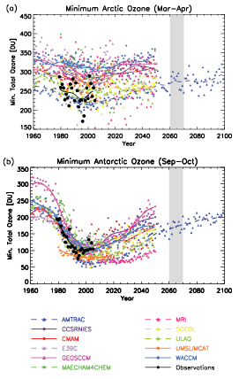
Figure 7.18. (a) Minimum arctic total column ozone for March to April and (b) minimum antarctic total column ozone for September to October (both poleward of 60°) in Dobson Units (DU). Simulations of future evolution of ozone were performed by 11 CCMs analysed as part of the CCM Validation Activity for SPARC (http://www.pa.op.dlr.de/CCMVal/). Model results are compared with values calculated from the National Institute of Water and Atmospheric Research (NIWA) assimilated total column ozone database shown as black dots ( Bodeker et al., 2005 [ARC] ). The light grey shading between 2060 and 2070 shows the period when halogen amounts in the polar lower stratosphere are expected to return to 1980 values. Models include AMTRAC: Atmospheric Model with Transport and Chemistry; CCSRNIES: Center for Climate System Research - National Institute for Environmental Studies; CMAM: Canadian Middle Atmosphere Model; E39C: German Aerospace Center (DLR) version of ECHAM4 with chemistry and 39 levels; GEOSCCM: Goddard Earth Observing System Chemistry-Climate Model; MAECHAM4/CHEM: Middle Atmosphere ECHAM4 with Chemistry; MRI: Meteorological Research Institute; SOCOL: Solar Climate Ozone Links; ULAQ: University of L’Aquila; UMSLIMCAT: Unified Model SLIMCAT; WACCM: Whole Atmosphere Community Climate Model.
7.4.6.4 Uncertainties Due to Atmospheric Dynamics
Changes in atmospheric dynamics could affect ozone. For example, sub-grid scale processes such as gravity wave propagation (e.g., Warner and McIntyre, 2001 [JoC] ), prescribed for past and present conditions, may change in the future. Tropospheric climate changes will also alter planetary-scale waves. Together with changes in orographic gravity waves, these waves give rise to the increase in the Brewer-Dobson circulation seen in most models ( Butchart et al., 2006 [NPR, JoC, MoS] ). The magnitude of this effect varies from model to model and leads to increased adiabatic heating of the polar regions, compensating in part the increased radiative cooling from CO2 increases. Hence, the net heating or cooling is subject to large uncertainty, and available model simulations do not give a consistent picture of future development of ozone, particularly in the Arctic( Figure 7.18 ).
7.5 Aerosol Particles and the Climate System
Aerosols are an integral part of the atmospheric hydrological cycle and the atmosphere’s radiation budget, with many possible feedback mechanisms that are not yet fully understood. This section assesses (1) the impact of meteorological (climatic) factors like wind, temperature and precipitation on the natural aerosol burden and (2) possible effects of aerosols on climate parameters and biogeochemistry. The most easily understood interaction between aerosols and climate is the direct effect (scattering and absorption of shortwave and thermal radiation), which is discussed in detail in Chapter2 .Interactions with the hydrological cycle, and additional impacts on the radiation budget, occur through the role of aerosols in cloud microphysical processes, as aerosol particles act as cloud condensation nuclei (CCN) and ice nuclei (IN). The suite of possible impacts of aerosols through the modification of cloud properties is called ‘indirect effects’. The forcing aspect of the indirect effect at the top of the atmosphere is discussed in Chapter2 ,while the processes that involve feedbacks or interactions, like the ‘cloud lifetime effect’ [6] ,the ‘semi-direct effect’ and aerosol impacts on the large-scale circulation, convection, the biosphere through nutrient supply and the carbon cycle, are discussed here.
7.5.1 Aerosol Emissions and Burdens Affected by Climatic Factors
Most natural aerosol sources are controlled by climatic parameters like wind, moisture and temperature. Hence, human-induced climate change is also expected to affect the natural aerosol burden. The sections below give a systematic overview of the major natural aerosol sources and their relations to climate parameters while anthropogenic aerosol emissions and combined aerosols are the subject of Chapter2 .
7.5.1.1 Dust
Estimates of the global source strength of bulk dust aerosols with diameters below 10 µm of between 1,000 and 3,000 Tg yr–1 agree well with a wide range of observations ( Duce, 1995 [NPR, MoS] ; Textor et al., 2005 [ARC] ; Cakmur et al., 2006 [NPR, JoC, MoS] ). Seven to twenty percent of the dust emissions are less than 1 µm in diameter ( Cakmur et al., 2006 [NPR, JoC, MoS] ; Schulz et al., 1998 [JoC, MoS, SRC] Zhang et al. 1997 [JoC] ) estimated that about 800 Tg yr–1 of Asian dust emissions are injected into the atmosphere annually, about 30% of which is re-deposited onto the deserts and 20% is transported over regional scales, while the remaining approximately 50% is subject to long-range transport to the Pacific Ocean and beyond. Asian dust appears to be a continuous source that dominates background dust aerosol concentrations on the west coast of the USA ( Duce, 1995 [NPR, MoS] ; Perry et al., 2004 [JoC] ). Uncertainties in the estimates of global dust emissions are greater than a factor of two ( Zender et al., 2004 [JoC, MoS] ) due to problems in validating and modelling the global emissions. The representation of the high wind tail of the wind speed distribution alone, responsible for most of the dust flux, leads to differences in emissions of more then 30% ( Timmreck and Schulz, 2004 [JoC, MoS, SRC] ). Observations suggest that annual mean African dust may have varied by a factor of four during 1960 to 2000 ( Prospero and Lamb, 2003 [JoC] ), possibly due to rainfall variability in the Sahel zone. Likewise, simulations of dust emissions in 2100 are highly uncertain, ranging from a 60% decrease to a factor of 3.8 increase as compared to present-day dust emissions ( Mahowald and Luo, 2003 [JoC, MoS] ; Tegen et al., 2004 [JoC, MoS] ; Woodward et al., 2005 [JoC, MoS, SRC] ; Stier et al., 2006a [MoS] ). Reasons for these discrepancies include different treatments of climate-biosphere interactions and the climate model used to drive the vegetation and dust models. The potentially large impact of climate change on dust emissions shows up in particular when comparing present-day with LGM conditions for dust erosion (e.g., Werner et al., 2002 [JoC] ).
The radiative effect of dust, which, for example, could intensify the African Easterly Waves, may be a feedback mechanism between climate and dust ( Jones et al., 2004 [NPR, JoC, SRC] ). It also alters the atmospheric circulation, which feeds back to dust emission from natural sources (see Section 7.5.4 Perlwitz et al. 2001 [JoC, MoS] ) estimate that this feedback reduces the global dust load by roughly 15%, as dust radiative forcing reduces the downward mixing of momentum within the planetary boundary layer, the surface wind speed, and thus dust emission ( Miller et al., 2004a [JoC, MoS] ). In addition to natural dust production, human activities have created another potential source for dust mobilisation through desertification. The contribution to global dust emission of desertification through human activities is uncertain: estimates vary from 50% ( Tegen et al., 1996 [JoC, MoS, SRC] ; Mahowald et al., 2004 [JoC, MoS] ) to less than 10% ( Tegen et al., 2004 [JoC, MoS] ) to insignificant values ( Ginoux et al., 2001 [JoC, MoS] ; Prospero et al., 2002 [JoC] ). A 43-year estimate of Asian dust emissions reveals that meteorology and climate have a greater influence on Asian dust emissions and associated Asian dust storm occurrences than does desertification( Figure 7.19 ;Zhang et al., 2003 [JoC] ).
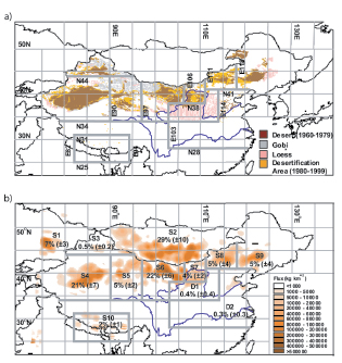
Figure 7.19. (a) Chinese desert distributions from 1960 to 1979 and desert plus desertification areas from 1980 to 1999 . (b) Sources (S1 to S10) and typical depositional areas (D1 and D2) for Asian dust indicated by spring average dust emission flux (kg km–2 per month) averaged over 1960 to 2002 . The percentages with standard deviations in parentheses denote the average amount of dust production in each source region and the total amount of emissions between 1960 and 2002 . The deserts in Mongolia (S2) and in western (S4) and northern (S6) China (mainly the Taklimakan and Badain Juran, respectively) can be considered the major sources of Asian dust emissions. Several areas with more expansions of deserts (S7, S8, S9 and S5) are not key sources. Adapted from Zhang et al. 2003 [JoC] ).
In addition, aerosol deposition affects global ecosystems. Deposition of mineral dust plays an important role in the biogeochemical cycle of the oceans, by providing the nutrient iron, which affects ocean biogeochemistry with feedbacks to climate and dust production ( Jickells et al., 2005 [JoC] ; Section 7.3.4.4 ). Conversely, water-soluble particulate iron over the Pacific Ocean is linked to elemental carbon emissions resulting from anthropogenic activity in Asia ( Chuang et al., 2005 [NPR, JoC] ). The input of trace elements by dust deposition is also of importance to terrestrial ecosystems. For example, it has been proposed that the vegetation of the Amazon basin is highly dependent on Saharan dust deposition, which provides phosphorus, necessary for maintenance of long-term productivity ( Okin et al., 2004 [JoC, ARC] ; Section 7.3 ). The Hawaiian Islands also depend on phosphorus from Asian dust transport ( Chadwick et al., 1999 [JoC] ). Moreover, mineral dust can act as a sink for acidic trace gases, such as sulphur dioxide (SO2)and HNO3,and thereby interact with the sulphur and N cycles (e.g., Dentener et al., 1996 [JoC, SRC] ; Umann et al., 2005 [JoC] ). Coatings with soluble substances, such as sulphate or nitrate, will change the ability of mineral dust aerosols to nucleate cloud droplets ( Levin et al., 1996 [JoC] ; Section 7.5.2.1 ).
7.5.1.2 Sea Salt
Sea salt aerosol is a key aerosol constituent of the marine atmosphere. Sea salt aerosol particles affect the formation of clouds and rain. They serve as sinks for reactive gases and small particles and possibly suppress new particle formation. Sea salt is also responsible for a large fraction of the non-sea salt sulphate formation (e.g., Sievering et al., 1992 [JoC] ). The major meteorological and environmental factors that affect sea salt formation are wind speed, atmospheric stability and wind friction velocity, sea surface and air temperatures, present and prior rain or snow and the amount and nature of surface-active materials in the near-surface ocean waters ( Lewis and Schwartz, 2005 [NPR, MoS, SRC] ). The average annual global sea salt flux from 12 models is estimated to be 16,300 Tg ± 200% ( Textor et al., 2005 [ARC] ) of which 15% is emitted into the submicron mode.
New evidence shows that the ocean also acts as a source of organic matter from biogenic origin ( O’Dowd et al., 2004 [JoC] ; Leck and Bigg, 2005b [JoC, SRC] O’Dowd et al. 2004 [JoC] ) show that during phytoplankton blooms (summer conditions), the organic aerosols can constitute up to 63% of the total aerosol. Surface-active organic matter of biogenic origin (such as lipidic and proteinaceous material and humic substances), enriched in the oceanic surface layer and transferred to the atmosphere by bubble-bursting processes, are the most likely candidates to contribute to the observed organic fraction in marine aerosol. Insoluble heat-resistant organic sub-micrometre particles (peaking at 40 to 50 nm in diameter), mostly combined into chains or aggregated balls of ‘marine microcolloids’ linked by an amorphous electron-transparent material with properties entirely consistent with exopolymer secretions ( (Decho, 1990; ) ( Verdugo et al., 2004 ) ), are found in near-surface water of lower-latitude oceans ( Benner et al., 1992 [JoC] ;( Wells and Goldberg, 1994 ) ), in leads between ice floes ( Bigg et al., 2004 [SRC] ), above the arctic pack ice ( Leck and Bigg, 2005a [JoC, SRC] ) and over lower-latitude oceans ( Leck and Bigg, 2005b [JoC, SRC] ). This aerosol formation pathway may constitute an ice (microorganisms)-ocean-aerosol-cloud feedback.
7.5.1.3 Natural Organic Carbon
Biogenic organic material is both directly emitted into the atmosphere and produced by VOCs. Primary emissions from the continents have been thought to be a relatively minor source but some studies suggest that these emissions could be much higher than previously estimated ( Folberth et al., 2005 [JoC, SRC] ; Jaenicke, 2005 [JoC] Kanakidou et al. 2005 [MoS] ) estimate a global biogenic secondary organic aerosol production of about 30 Tg yr–1 and recognise the potentially large, but uncertain, flux of primary biogenic particles. Annual global biogenic VOC emission estimates range from 500 to 1,200 Tg yr–1 ( Guenther et al., 1995 [JoC, MoS, SRC] ). There is a large range (less than 5 to greater than 90%) of organic aerosol yield for individual compounds and atmospheric conditions resulting in estimates of global annual secondary organic aerosol production from biogenic VOCs that range from 2.5 to 44.5 Tg of organic matter per year ( Tsigaridis and Kanakidou, 2003 [MoS] ). All biogenic VOC emissions are highly sensitive to changes in temperature, and some emissions respond to changes in solar radiation and precipitation ( Guenther et al., 1995 [JoC, MoS, SRC] ). In addition to the direct response to climatic changes, biogenic VOC emissions are also highly sensitive to climate-induced changes in plant species composition and biomass distributions.
Global biogenic VOC emissions respond to climate change (e.g., ( Turner et al., 1991; ) Adams et al., 2001 [MoS, SRC] ; Penner et al., 2001 [NPR, ARC] ; Sanderson et al., 2003b [JoC] ). These model studies predict that solar radiation and climate-induced vegetation change can affect emissions, but they do not agree on the sign of the change. Emissions are predicted to increase by 10% per °C ( Guenther et al., 1993 [JoC, MoS, SRC] ). There is evidence of physiological adaptation to higher temperatures that would lead to a greater response for long-term temperature changes ( Guenther et al., 1999 [JoC, MoS, SRC] ). The response of biogenic secondary organic carbon aerosol production to a temperature change, however, could be considerably lower than the response of biogenic VOC emissions since aerosol yields can decrease with increasing temperature. A potentially important feedback among forest ecosystems, greenhouse gases, aerosols and climate exists through increased photosynthesis and forest growth due to increasing temperatures and CO2 fertilization ( (Kulmala et al., 2004 ) ). Increased forest biomass would increase VOC emissions and thereby organic aerosol production. This couples the climate effect of CO2 with that of aerosols.
7.5.1.4 Aerosols from Dimethyl Sulphide
Dimethyl sulphide produced by phytoplankton is the most abundant form in which the ocean releases gaseous sulphur. Sea-air fluxes of DMS vary by orders of magnitude depending mainly on DMS sea surface concentration and on wind speed. Estimates of the global DMS flux vary widely depending mainly on the DMS sea surface climatology utilised, sea-air exchange parametrization and wind speed data, and range from 16 to 54 Tg yr–1 of sulphur (see Kettle and Andreae, 2000 [JoC, MoS] for a review). According to model studies ( Gondwe et al., 2003 [JoC] ; Kloster et al., 2006 [MoS] ), 18 to 27% of the DMS is converted into sulphate aerosols. Penner et al. 2001 [NPR, ARC] ) show a small increase in DMS emissions between 2000 and 2100 (from 26.0 to 27.7 Tg yr–1 of sulphur) using constant DMS sea surface concentrations together with a constant monthly climatological ice cover. Gabric et al. 2004 [JoC, MoS] ) predict an increase of the globally integrated DMS flux perturbation of 14% for a tripling of the pre-industrial atmospheric CO2 concentration.
Bopp et al. 2004 [MoS] ) estimate the feedback of DMS to cloud albedo with a coupled atmosphere-ocean-biogeochemical climate model that includes phytoplankton species in the ocean and a sulphur cycle in the atmospheric climate model. They obtain an increase in the sea-air DMS flux of 3% for doubled atmospheric CO2 conditions, with large spatial heterogeneities (–15 to +30%). The mechanisms affecting those fluxes are marine biology, relative abundance of phytoplankton types and wind intensity. The simulated increase in fluxes causes an increase in sulphate aerosols and, hence, cloud droplets resulting in a radiative perturbation of cloud albedo of –0.05 Wm–2,which represents a small negative climate feedback to global warming.
7.5.1.5 Aerosols from Iodine Compounds
Intense new aerosol particle formation has been frequently observed in the coastal environment ( O’Dowd et al., 2002a [JoC] ). Simultaneous coastal observations of reactive iodine species ( Saiz-Lopez et al., 2005 [MoS] ), chamber studies using iodocarbon precursors and laboratory characterisation of iodine oxide particles formed from exposure of Laminaria macroalgae to ozone ( McFiggans et al., 2004 [SRC] ) have demonstrated that coastal particle formation is linked to iodine compound precursor released from abundant infralittoral beds of macroalgae. The particle bursts overwhelmingly occur during daytime low tides ( O’Dowd et al., 2002b [JoC] ; Saiz-Lopez et al., 2005 [MoS] ). Tidal exposure of kelp leads to the well-documented release of significant fluxes of iodocarbons ( (Carpenter et al., 2003 ) ), the most photolabile of which, di-iodomethane (CH2I2), may yield a high iodine atom flux. However, the iodine monoxide (IO) and iodine dioxide (OIO) radicals, and new particles are thought more likely to result from emissions of molecular iodine ( McFiggans et al., 2004 [SRC] ), which will yield a much greater iodine atom flux ( Saiz-Lopez and Plane, 2004 [JoC] ). It is unclear whether such particles grow sufficiently to act as CCN ( O’Dowd, 2002 [JoC] ; Saiz-Lopez et al., 2005 [MoS] ). Thus, a hitherto undiscovered remote ocean source of iodine atoms (such as molecular iodine) must be present if iodine-mediated particle formation is to be important in the remote marine boundary layer ( McFiggans, 2005 [JoC, SRC] ).
Aerosol burden and lifetime are also affected by microphysical interactions among the different aerosol compounds as well as by changes in the spatial and seasonal distribution of the emissions. Sea salt aerosols, for example, provide surfaces for conversion of SO2 into sulphate aerosols ( Sievering et al., 1992 [JoC] ) with consequences for cloud formation ( Gong and Barrie, 2003 [JoC, MoS] ; Section 7.5.2.1 ). A future reduction in SO2 emissions and the associated reduced conversion of hydrophobic to hydrophilic soot could lead to a prolonged residence time of soot ( Cooke et al., 2002 [JoC, MoS, ARC] ; Stier et al., 2006b [JoC, MoS] ) and increased ammonium nitrate ( Liao and Seinfeld, 2005 [JoC, MoS] ). However, in a transient AOGCM climate simulation with an em-bedded microphysical aerosol module, Stier et al. 2006a [MoS] ) show that the effect on the hydrophobic to hydrophilic conversion can be outweighed by a general shift to low-latitude dry-season soot emissions. Consequently, soot lifetime increases in a future climate despite an enhanced conversion of hydrophobic to hydrophilic soot.
7.5.1.6 Climatic Factors Controlling Aerosol Burdens and Cycling
As discussed above, near-surface wind speed determines the source strength for primary aerosols (sea salt, dust, primary organic particles) and precursors of secondary aerosols (mainly DMS). Progress has been made in the development of source functions (in terms of wind speed) for sea salt and desert dust (e.g., Tegen et al., 2002 [JoC, MoS] ; Gong, 2003 [JoC] ; Balkanski et al., 2004 [NPR] ). Wind speed also affects dry deposition velocities and hence the lifetime of aerosols. In addition, biogenic emissions are strongly dependent on temperature (together with humidity/moisture; e.g., Guenther et al., 1995 [JoC, MoS, SRC] ). Temperature also is a key factor in the gas-aerosol partitioning of semi-volatile secondary organics ( Kanakidou et al., 2005 [MoS] ).
Precipitation directly affects the wet removal and hence the lifetime of atmospheric aerosols. More aerosols decrease the precipitation formation rate, which in turn increases the lifetime of aerosols and results in more long-range aerosol transport to remote regions where wet removal is less efficient. At the same time, precipitating boundary layer clouds maintain themselves by keeping aerosol concentrations low (e.g., Baker and Charlson, 1990 [JoC] ; Stevens et al., 2005 [JoC] ; Sharon et al., 2006 [JoC] ). Precipitation also affects soil moisture, with impacts on dust source strength and on stomatal opening/closure of plant leaves, hence affecting biogenic emissions. Cloud processing is an important pathway in the gas-to-particle conversion. It is the most important oxidation pathway for sulphate aerosols and shifts the aerosol size distribution to larger sizes, such that aerosols are more easily activated in subsequent cloud events (e.g., Hoppel et al., 1990 [JoC] ; Kerkweg et al., 2003 [JoC, MoS] ; Yin et al., 2005 [JoC] ). It is also important in the conversion of hydrophobic to hydrophilic carbon.
7.5.2 Indirect Effects of Aerosols on Clouds and Precipitation
Aerosols can interact with clouds and precipitation in many ways, acting either as CCN or IN, or as absorbing particles, redistributing solar energy as thermal energy inside cloud layers. These indirect effects (in contrast to the direct interaction with radiation, see Chapter2 )are the subject of this subsection. They can be subdivided into different contributing processes, as summarised in Table 7.10 and shown in Figure 7.20 .Cloud feedbacks remain the largest source of uncertainty in climate sensitivity estimates and the relatively poor simulation of boundary layer clouds in the present climate is a reason for some concern (see Chapter8 ). Therefore the results discussed below need to be considered with caution.
Table 7.10a. Overview of the different aerosol indirect effects and their sign of the net radiative flux change at the top of the atmosphere (TOA).
Table 7.10b. Overview of the different aerosol indirect effects and their implications for the global mean net shortwave radiation at the surface,Fsfc (Columns 2-4) and for precipitation (Columns 5-7).
| Effect | Cloud Types Affected | Process | Sign of Change in TOA Radiation | Potential Magnitude | Scientific Understanding |
|---|---|---|---|---|---|
| Cloud albedo effect | All clouds | For the same cloud water or ice content more but smaller cloud particles reflect more solar radiation | Negative | Medium | Low |
| Cloud lifetime effect | All clouds | Smaller cloud particles decrease the precipitation efficiency thereby presumably prolonging cloud lifetime | Negative | Medium | Very low |
| Semi-direct effect | All clouds | Absorption of solar radiation by absorbing aerosols affects static stability and the surface energy budget, and may lead to an evaporation of cloud particles | Positive or negative | Small | Very low |
| Glaciation indirect effect | Mixed-phase clouds | An increase in IN increases the precipitation efficiency | Positive | Medium | Very low |
| Thermodynamic effect | Mixed-phase clouds | Smaller cloud droplets delay freezing causing super-cooled clouds to extend to colder temperatures | Positive or negative | Medium | Very low |
| Effect | Sign of Change inFsfc | Potential Magnitude | Scientific Understanding | Sign of Change in Precipitation | Potential Magnitude | Scientific Understanding |
|---|---|---|---|---|---|---|
| Cloud albedo effect | Negative | Medium | Low | n.a. | n.a. | n.a. |
| Cloud lifetime effect | Negative | Medium | Very low | Negative | Small | Very low |
| Semi-direct effect | Negative | Large | Very low | Negative | Large | Very low |
| Glaciation indirect effect | Positive | Medium | Very low | Positive | Medium | Very low |
| Thermodynamic effect | Positive or negative | Medium | Very low | Positive or negative | Medium | Very low |
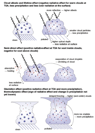
Figure 7.20. Schematic diagram of the aerosol effects discussed in Table 7.10 .TOA refers to the top-of-the-atmosphere.
The cloud-albedo effect, that is, the distribution of the same cloud liquid water content over more, hence smaller, cloud droplets leading to higher cloud reflectivity, is a purely radiative forcing and is therefore treated in Chapter2 .The other effects involve feedbacks in the climate system and are discussed here. The albedo effect cannot be easily separated from the other effects; in fact, the processes that decrease the cloud droplet size per given liquid water content also decrease precipitation formation, presumably prolonging cloud lifetime (cloud lifetime effect, Section 7.5.2.1 and Figure 7.20 ). In turn, an increase in cloud lifetime also contributes to a change in the time-averaged cloud albedo. The semi-direct effect refers to the absorption of solar radiation by soot, re-emitted as thermal radiation, hence heating the air mass and increasing static stability relative to the surface. It may also cause evaporation of cloud droplets (see Sections 2.4 and 7.5.4.1 and Figure 7.20 ). The glaciation effect refers to an increase in IN resulting in a rapid glaciation of a super-cooled liquid water cloud due to the difference in vapour pressure over ice and water. Unlike cloud droplets, these ice crystals grow in an environment of high super-saturation with respect to ice, quickly reaching precipitation size, with the potential to turn a non-precipitating cloud into a precipitating cloud( Section 7.5.2.2 and Figure 7.20 ). The thermodynamic effect refers to a delay in freezing by the smaller droplets causing super-cooled clouds to extend to colder temperatures( Section 7.5.2.2 and Figure 7.20 ). In addition to aerosol-induced changes at the top of the atmosphere (TOA), aerosols affect the surface energy budget( Table 7.10 b; Section 7.5.2 )with consequences for convection, evaporation and precipitation( Figure 7.20 ).
7.5.2.1 Aerosol Effects on Water Clouds and Warm Precipitation
Aerosols are hypothesised to increase the lifetime of clouds because increased concentrations of smaller droplets lead to decreased drizzle production and reduced precipitation efficiency ( Albrecht, 1989 [JoC] ). It is difficult to devise observational studies that can separate the cloud lifetime from the cloud albedo effect (see Section 2.4 ). Thus, observational studies usually provide estimates of the combined effects. Similarly, climate models cannot easily separate the cloud lifetime indirect effect once the aerosol scheme is fully coupled to a cloud microphysics scheme, but also predict the combined cloud albedo, lifetime and semi-direct effect.
Evidence for the absence of a drizzle mode due to anthropogenic emissions of aerosols and their precursors comes, for instance, from ship tracks perturbing marine stratus cloud decks off the coast of California ( Ferek et al., 1998 [JoC] ) as well as from analysing polluted compared with clean clouds off the Atlantic coast of Canada ( Peng et al., 2002 [JoC] ). One problem is that most climate models suggest an increase in liquid water when adding anthropogenic aerosols, whereas newer ship track studies show that polluted marine water clouds can have less liquid water than clean clouds ( Platnick et al., 2000 [JoC] ; Coakley and Walsh, 2002 [JoC, MoS] Ackerman et al. 2004 [JoC, MoS] ) attribute this effect to enhanced entrainment of dry air in polluted clouds in these instances with subsequent evaporation of cloud droplets. Similarly, when cloud lifetime is analysed, an increase in aerosol concentration from very clean to very polluted does not increase cloud lifetime, even though precipitation is suppressed ( Jiang et al., 2006 [NPR, JoC] ). This effect is due to competition between precipitation suppression and enhanced evaporation of the more numerous smaller cloud droplets in polluted clouds. Observed lower aerosol concentrations in pockets of open cells ( Stevens et al., 2005 [JoC] ) and in rifts of broken clouds surrounded by solid decks of stratocumulus with higher aerosol concentrations ( Sharon et al., 2006 [JoC] ) are manifestations of two stable aerosol regimes ( Baker and Charlson, 1990 [JoC] ). The low aerosol concentration regimes maintain themselves by higher drizzle rates. However, it is hard to disentangle cause and effect from these studies.
Smoke from burning vegetation reduces cloud droplet sizes and delays the onset of precipitation ( Warner and Twomey, 1967 [JoC] ; Rosenfeld, 1999 [JoC] ; Andreae et al., 2004 [JoC] ). In addition, desert dust suppresses precipitation in thin low-altitude clouds ( Rosenfeld et al., 2001 [JoC] ; Mahowald and Kiehl, 2003 [NPR, JoC] ). Contradictory results have been found regarding the suppression of precipitation by aerosols downwind of urban areas ( Givati and Rosenfeld, 2004 [JoC] ; Jin et al., 2005 [JoC, ARC] ) and in Australia ( Rosenfeld, 2000 [JoC] ;( Ayers, 2005 ) ).
Models suggest that anthropogenic aerosols suppress precipitation in the absence of giant CCN and aerosol-induced changes in ice microphysics (e.g., Lohmann, 2002 [NPR, JoC, SRC] ; Menon and DelGenio, 2007 ) as well as in mixed-phase clouds where the ice phase only plays a minor role ( Phillips et al., 2002 [JoC] ). A reduction in precipitation formation leads to increased cloud processing of aerosols. Feingold et al. 1998 [JoC, MoS] and Wurzler et al. 2000 [JoC] ) showed that cloud processing could either lead to an increase or decrease in precipitation formation in subsequent cloud cycles, depending on the size and concentration of activated CCN. Giant sea salt nuclei, on the other hand, may override the precipitation suppression effect of the large number of small pollution nuclei ( Johnson, 1982 [JoC] ; Feingold et al., 1999 [JoC] ; Rosenfeld et al., 2002 [JoC] ). Likewise, Gong and Barrie 2003 [JoC, MoS] ) predict a reduction of 20 to 60% in marine cloud droplet number concentrations and an increase in precipitation when interactions of sulphate with sea salt aerosols are considered. When aerosol effects on warm convective clouds are included in addition to their effect on warm stratiform clouds, the overall indirect aerosol effect and the change in surface precipitation can be larger or smaller than if just the aerosol effect on stratiform clouds is considered ( Nober et al., 2003 [JoC] ; Menon and Rotstayn, 2006 [JoC, MoS, SRC] ). Besides changes in the distribution of precipitation, the frequency of extreme events may also be reduced by the presence of aerosols ( Paeth and Feichter, 2006 [JoC, MoS, SRC] ).
Observations show that aerosols can decrease or increase cloud cover. Kaufman et al. 2005 [JoC] ) conclude from satellite observations that the aerosol indirect effect is likely primarily due to an increase in cloud cover, rather than an increase in cloud albedo. In contrast, model results of Lohmann et al. 2006 [Ambiguous] ) associate the increase in cloud cover with differing dynamic regimes and higher relative humidities that maintain higher aerosol optical depths. On the other hand, the semi-direct effect of absorbing aerosols can cause evaporation of cloud droplets and/or inhibit cloud formation. In a large area with absorbing biomass-burning aerosol, few low-lying clouds were observed when the aerosol optical depth exceeded 1.2 ( Koren et al., 2004 [JoC] ). Increasing emissions of absorbing aerosols from the late 1980 s to the late 1990 s in China also reduced cloud amount leading to a decrease in local planetary albedo, as deduced from satellite data ( Krüger and Grassl, 2004 [NPR, JoC] ). When the combined effect of pollution and smoke aerosols is considered from ground-based observations, the net effect seems to be an increase in cloud cover with increasing aerosol column concentrations ( Kaufman and Koren, 2006 [JoC] ).
7.5.2.2 Aerosol Impacts on Mixed-Phase Clouds
As satellite observations of aerosol effects on mixed-phase clouds are not conclusive ( Mahowald and Kiehl, 2003 [NPR, JoC] ), this section only refers to model results and field studies. Studies with GCMs suggest that if, in addition to mineral dust, hydrophilic black carbon aerosols are assumed to act as IN at temperatures between 0°C and –35°C, then increases in aerosol concentration from pre-industrial to present times may cause a glaciation indirect effect ( Lohmann, 2002 [NPR, JoC, SRC] ). Increases in IN can result in more frequent glaciation of super-cooled stratiform clouds and increase the amount of precipitation via the ice phase, which could decrease the global mean cloud cover leading to more absorption of solar radiation. Whether the glaciation effect or warm cloud lifetime effect is larger depends on the chemical nature of the dust ( Lohmann and Diehl, 2006 [JoC, SRC] ). Likewise, the number and size of ice particles in convective mixed-phase clouds is sensitive to the chemical composition of the insoluble fraction (e.g., dust, soot, biological particles) of the aerosol particles ( Diehl and Wurzler, 2004 [JoC, MoS] ).
Rosenfeld 1999 [JoC] and Rosenfeld and Woodley 2000 [JoC] ) analysed aircraft data together with satellite data suggesting that pollution aerosols suppress deep convective precipitation by decreasing cloud droplet size and delaying the onset of freezing. This hypothesis was supported by a cloud-resolving model study ( Khain et al., 2001 [JoC, MoS] ) showing that super-cooled cloud droplets down to –37.5°C could only be simulated if the cloud droplets were small and numerous. Precipitation from single-cell mixed-phase convective clouds is reduced under continental and maritime conditions when aerosol concentrations are increased ( (Yin et al., 2000; ) Khain et al., 2004 [JoC, MoS] ; Seifert and Beheng, 2006 [NPR] ). In the modelling study by Cui et al. 2006 [JoC] ), this is caused by drops evaporating more rapidly in the high aerosol case (see also Jiang et al., 2006 [NPR, JoC] ), which eventually reduces ice mass and hence precipitation. Khain et al. 2005 [JoC] ) postulate that smaller cloud droplets, such as those originating from human activity, would change the thermodynamics of convective clouds. More, smaller droplets would reduce the production of rain in convective clouds. When these droplets freeze, the associated latent heat release would then result in more vigorous convection and more precipitation. In a clean cloud, on the other hand, rain would have depleted the cloud so that less latent heat is released when the cloud glaciates, resulting in less vigorous convection and less precipitation. Similar results were obtained by Koren et al. 2005 [JoC] Zhang et al. 2005 [NPR, JoC, MoS, SRC] ) and for the multi-cell cloud systems studied by Seifert and Beheng 2006 [NPR] ). For a thunderstorm in Florida in the presence of Saharan dust, the simulated precipitation enhancement only lasted two hours after which precipitation decreased as compared with clean conditions ( van den Heever et al., 2006 [JoC, MoS] ). Cloud processing of dust particles, sulphate particles and trace gases can lead to an acceleration of precipitation formation in continental mixed-phase clouds, whereas in maritime clouds, which already form on rather large CCN, the simulated effect on precipitation is small ( Yin et al., 2002 [NPR, JoC] ). This highlights the complexity of the system and indicates that the sign of the global change in precipitation due to aerosols is not yet known. Note that microphysical processes can only change the temporal and spatial distribution of precipitation while the total amount of precipitation can only change if evaporation from the surface changes.
7.5.2.3 Aerosol Impacts on Cirrus Clouds
Cirrus clouds can form by homogeneous and heterogeneous ice nucleation mechanisms at temperatures below 235 K. While homogeneous freezing of super-cooled aqueous phase aerosol particles is rather well understood, understanding of heterogeneous ice nucleation is still in its infancy. A change in the number of ice crystals in cirrus clouds could exert a cloud albedo effect in the same way that the cloud albedo effect acts for water clouds. In addition, a change in the cloud ice water content could exert a radiative effect in the infrared. The magnitude of these effects in the global mean has not yet been fully established, but the development of physically based parametrization schemes of cirrus formation for use in global models led to significant progress in understanding underlying mechanisms of aerosol-induced cloud modifications ( Kärcher and Lohmann, 2002 [NPR, JoC, SRC] ; Liu and Penner, 2005 [MoS, ARC] ; Kärcher et al., 2006 [NPR, JoC, MoS, SRC] ).
Aglobal climate model study concluded that a cloud albedo effect based solely on ubiquitous homogeneous freezing is small globally ( Lohmann and Kärcher, 2002 [NPR, JoC, MoS, SRC] ). This is expected to also hold in the presence of heterogeneous IN that cause cloud droplets to freeze at relative humidities over ice close to homogeneous values (above 130–140%) ( Kärcher and Lohmann, 2003 [NPR, JoC, SRC] ). Efficient heterogeneous IN, however, would be expected to lower the relative humidity over ice, so that the climate effect may be larger ( Liu and Penner, 2005 [MoS, ARC] ). In situ measurements reveal that organic-containing aerosols are less abundant than sulphate aerosols in ice cloud particles, suggesting that organics do not freeze preferentially ( Cziczo et al., 2004 [NPR, JoC] ). A model study explains this finding by the disparate water uptake of organic aerosols, and suggests that organics are unlikely to significantly modify cirrus formation unless they are present in very high concentrations (compared with sulphate-rich particles) at low temperatures ( Kärcher and Koop, 2004 [SRC] ).
With regard to aerosol effects on cirrus clouds, a strong link has been established between gravity wave induced, mesoscale variability in vertical velocities and climate forcing by cirrus ( Kärcher and Ström, 2003 [SRC] ; Hoyle et al., 2005 [JoC] ). Hemispheric-scale studies of aerosol-cirrus interactions using ensemble trajectories suggest that changes in upper-tropospheric cooling rates and ice-forming aerosols in a future climate may induce changes in cirrus occurrence and optical properties that are comparable in magnitude with observed decadal trends in global cirrus cover ( Haag and Kärcher, 2004 [NPR, JoC, SRC] ). Optically thin and sub-visible cirrus are particularly susceptible to IN and therefore likely affected by anthropogenic activities.
Radiative forcing estimates and observed trends of aviation-induced cloudiness are discussed in Section 2.6 .In terms of indirect effects of aircraft-induced aerosols on cirrus clouds, Lohmann and Kärcher 2002 [NPR, JoC, MoS, SRC] ) show that the impact of aircraft sulphur emissions on cirrus properties via homogeneous freezing is small. The contribution from air traffic to the global atmospheric black carbon cycle was assessed by Hendricks et al. 2004 [MoS] ). Assuming that black carbon particles from aviation serve as efficient IN, maximum increases or decreases in ice crystal number concentrations of more than 40% are simulated in a climate model study assuming that the ‘background’ (no aviation impact) cirrus cloud formation is dominated by heterogeneous or homogeneous nucleation, respectively ( Hendricks et al., 2005 [JoC, SRC] ). Progress in assessing the impact of aircraft black carbon on cirrus is hampered by the poor knowledge of natural freezing modes in cirrus conditions and the inability to describe the full complexity of cirrus processes in global models.
7.5.2.4 Global Climate Model Estimates of the Total Anthropogenic Aerosol Effect
The total anthropogenic aerosol effect as defined here includes estimates of the direct effect, semi-direct effect, indirect cloud albedo and cloud lifetime effect for warm clouds from several climate models. The total anthropogenic aerosol effect is obtained as the difference between a multi-year simulation with present-day aerosol emissions and a simulation representative for pre-industrial conditions, where anthropogenic emissions are turned off. It should be noted that the representation of the cloud lifetime effect in GCMs is essentially one of changing the auto-conversion of cloud water to rainwater.
The global mean total anthropogenic aerosol effect on net radiation at TOA from pre-industrial times to the present day is shown in Figure 7.21 .Whereas Chapter2 only considers the radiative forcing of the cloud albedo effect, here feedbacks are included in the radiative flux change. In most simulations shown in Figures 7.21 to 7.23 ,the total aerosol effect is restricted to warm clouds except for the simulations by ( Jacobson 2006 ) and Lohmann and Diehl 2006 [JoC, SRC] ), who also include aerosol effects on mixed-phase and ice clouds. The total aerosol effect ranges from –0.2 Wm–2 in the combined GCM plus satellite simulations ( Quaas et al., 2006 [SRC] ) to –2.3 Wm–2 in the simulations by Ming et al. 2005 [JoC, MoS] ), with an average forcing of –1.2 Wm–2.The total aerosol effect is larger when sulphate aerosols are used as surrogates for all anthropogenic aerosols than if multiple aerosol types are considered( Figure 7.21 ). Although most model estimates also include the direct and semi-direct effects, their contribution to the TOA radiation is generally small compared with the indirect effect, ranging from +0.1 to –0.5 Wm–2 due to variations in the locations of black carbon with respect to the cloud ( Lohmann and Feichter, 2005 [SRC] ). The simulated cloud lifetime effect in a subset of models displayed in Figure 7.21 varies between –0.3 and –1.4 Wm–2 ( Lohmann and Feichter, 2005 [SRC] ), which highlights some of the differences among models. The importance of the cloud albedo effect compared with the cloud lifetime effect varies even when the models use the same aerosol fields ( Penner et al., 2006 [MoS, ARC] ). Other differences among the simulations include an empirical treatment of the relationship between aerosol mass and cloud droplet number concentration vs. a mechanistic relationship, the dependence of the indirect aerosol effect on the assumed background aerosol or cloud droplet number concentration, and the competition between natural and anthropogenic aerosols as CCN ( Ghan et al., 1998 [JoC] ; O’Dowd et al., 1999 [JoC, MoS, ARC] ). Likewise, differences in the cloud microphysics scheme, especially in the auto-conversion rate, cause different cloud responses (e.g., A. Jones et al., 2001 [Ambiguous] ; Menon et al., 2002a [JoC, MoS, SRC] , 2003; Penner et al., 2006 [MoS, ARC] ).
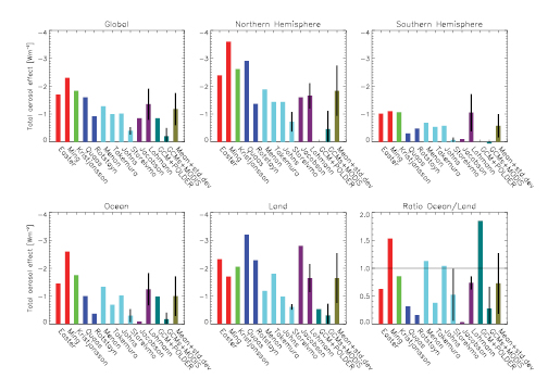
Figure 7.21. Global mean total anthropogenic aerosol effect (direct, semi-direct and indirect cloud albedo and lifetime effects) defined as the response in net radiation at TOA from pre-industrial times to the present day and its contribution over the NH and SH, over oceans and over land, and the ratio over oceans/land. Red bars refer to anthropogenic sulphate ( Easter et al., 2004 [JoC, MoS] ; Ming et al., 2005 [JoC, MoS] +), green bars refer to anthropogenic sulphate and black carbon ( Kristjánsson, 2002 [NPR, JoC] *,+), blue bars to anthropogenic sulphate and organic carbon ( Quaas et al., 2004 [JoC, MoS, SRC] ; Rotstayn and Liu, 2005 [JoC, MoS, SRC] +), turquoise bars to anthropogenic sulphate and black and organic carbon (Menon and del Genio, 2005 [NotFound] ; Takemura et al., 2005 [JoC, MoS, ARC] ; Johns et al., 2006 [JoC, MoS] ; Storelvmo et al., 2006 [JoC, MoS] ), dark purple bars to anthropogenic sulphate and black and organic carbon effects on water and ice clouds ( (Jacobson, 2006; ) Lohmann and Diehl, 2006 [JoC, SRC] ), teal bars refer to a combination of GCM and satellite results (European Centre for Medium Range Weather Forecasts/Max-Planck Institute for Meteorology Atmospheric GCM (ECHAM) plus Polarisation and Directionality of the Earth’s Reflectance (POLDER), Lohmann and Lesins, 2002 [JoC, SRC] ; Laboratoire de Météorologie Dynamique GCM (LMDZ)/ECHAM plus Moderate Resolution Imaging Spectroradiometer (MODIS), Quaas et al., 2006 [SRC] ) and olive bars to the mean and standard deviation from all simulations. Vertical black lines for individual results refer to ±1 standard deviation in cases of multiple simulations and/or results.
*refers to estimates of the aerosol effect deduced from the shortwave radiative flux only
+ refers to estimates solely from the indirect effects
All models agree that the total aerosol effect is larger over the NH than over the SH( Figure 7.21 ). The values of the NH total aerosol effect vary between –0.5 and –3.6 Wm–2 and in the SH between slightly positive and –1.1 Wm–2,with an average SH to NH ratio of 0.3. Estimates of the ocean/land partitioning of the total indirect effect vary from 0.03 to 1.8 with an average value of 0.7. While the combined European Centre for Medium Range Weather Forecasts/Max-Planck Institute for Meteorology Atmospheric GCM (ECHAM4) plus Polarisation and Directionality of the Earth’s Reflectance (POLDER) satellite estimate suggests that the total aerosol effect should be larger over oceans ( Lohmann and Lesins, 2002 [JoC, SRC] ), combined estimates of the Laboratoire de Météorologie Dynamique (LMD) and ECHAM4 GCMs with Moderate Resolution Imaging Spectroradiometer (MODIS) satellite data reach the opposite conclusion ( Quaas et al., 2006 [SRC] ). The average total aerosol effect over the ocean of –1 Wm–2 agrees with estimates of between –1 and –1.6 Wm–2 from the Advanced Very High Resolution Radiometer (AVHRR)/POLDER ( Sekiguchi et al., 2003 [JoC] ). Estimates from GCMs of the total aerosol effect are generally larger than those from inverse models ( Anderson et al., 2003 [JoC, MoS] and Chapter9 ).
As compared with the estimates of the total aerosol effect in Lohmann and Feichter 2005 [SRC] ), some new estimates ( Chen and Penner, 2005 [ARC] ; Rotstayn and Liu, 2005 [JoC, MoS, SRC] ; Lohmann and Diehl, 2006 [JoC, SRC] ) now also include the influence of aerosols on the cloud droplet size distribution (dispersion effect; Liu and Daum, 2002 [JoC, MoS] ). The dispersion effect refers to a widening of the size distribution in the polluted clouds that partly counteracts the reduction in the effective cloud droplet radius in these clouds. Thus, if the dispersion effect is taken into account, the indirect cloud albedo aerosol effect is reduced by 12 to 42% ( Peng and Lohmann, 2003 [JoC, SRC] ; Rotstayn and Liu, 2003 [JoC, SRC] ; Chen and Penner, 2005 [ARC] ). The global mean total indirect aerosol effect in the simulation by Rotstayn and Liu 2005 [JoC, MoS, SRC] ) has also been reduced due to a smaller cloud lifetime effect resulting from a new treatment of auto-conversion.
Global climate model estimates of the change in global mean precipitation due to the total aerosol effects are summarised in Figure 7.22 .Consistent with the conflicting results from detailed cloud system studies, the change in global mean precipitation varies between 0 and –0.13 mm day–1.These differences are amplified over the SH, ranging from –0.06 mm day–1 to 0.12 mm day–1.In general, the decreases in precipitation are larger when the atmospheric GCMs are coupled to mixed-layer ocean models (green bars), where the sea surface temperature and, hence, evaporation are allowed to vary.
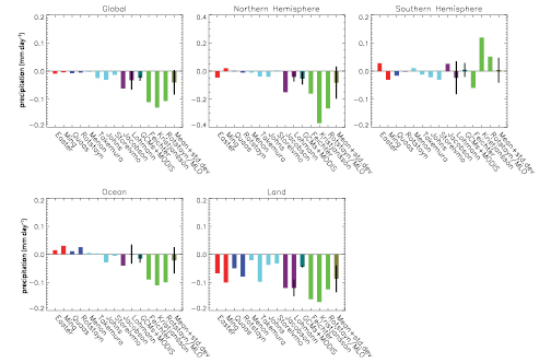
Figure 7.22. Global mean change in precipitation due to the total anthropogenic aerosol effect (direct, semi-direct and indirect cloud albedo and lifetime effects) from pre-industrial times to the present day and its contribution over the NH and SH, over oceans and over land. Red bars refer to anthropogenic sulphate ( Easter et al., 2004 [JoC, MoS] ; Ming et al., 2005 [JoC, MoS] +), blue bars to anthropogenic sulphate and organic carbon ( Quaas et al., 2004 [JoC, MoS, SRC] ; Rotstayn and Liu, 2005 [JoC, MoS, SRC] +), turquoise bars to anthropogenic sulphate, and black and organic carbon (Menon and del Genio, 2005 [NotFound] ; Takemura et al., 2005 [JoC, MoS, ARC] ; Johns et al., 2006 [JoC, MoS] ; Storelvmo et al., 2006 [JoC, MoS] ), dark purple bars to anthropogenic sulphate and black and organic carbon effects on water and ice clouds ( (Jacobson, 2006; ) Lohmann and Diehl, 2006 [JoC, SRC] ), teal bars refer to a combination of GCM and satellite results (LMDZ/ECHAM plus MODIS, Quaas et al., 2006 [SRC] ), green bars refer to results from coupled atmosphere/mixed-layer ocean (MLO) experiments ( Feichter et al., 2004 [JoC, MoS, SRC] : sulphate and black and organic carbon; Kristjansson et al., 2005 [JoC, MoS] : sulphate and black carbon; Rotstayn and Lohmann, 2002 [JoC, SRC] +:sulphate only) and olive bars to the mean from all simulations. Vertical black lines refer to ±1 standard deviation.
+ refers to estimates solely from the indirect effects
7.5.3 Effects of Aerosols and Clouds on Solar Radiation at the Earth’s Surface
By increasing aerosol and cloud optical depth, anthropogenic emissions of aerosols and their precursors contribute to a reduction of solar radiation at the surface. As such, worsening air quality contributes to regional aerosol effects. The partially conflicting observations on solar dimming/brightening are discussed in detail in Section 3.4 and Box 3.2 .This section focuses on the possible contribution by aerosols. The decline in solar radiation from 1961 to 1990 affects the partitioning between direct and diffuse solar radiation: Liepert and Tegen 2002 [NPR, JoC, MoS, ARC] ) concluded that over Germany, both aerosol absorption and scattering must have declined from 1975 to 1990 in order to explain the simultaneously weakened aerosol forcing and increased direct/diffuse solar radiation ratio. The direct/diffuse solar radiation ratio over the USA also increased from 1975 to 1990, likely due to increases in absorbing aerosols. Increasing aerosol optical depth associated with scattering aerosols alone in otherwise clear skies produces a larger fraction of diffuse radiation at the surface, which results in larger carbon assimilation into vegetation (and therefore greater transpiration) without a substantial reduction in the total surface solar radiation ( Niyogi et al., 2004 [JoC] ; Section 7.2.6.2).
For the tropical Indian Ocean, Ramanathan et al. 2001 [JoC, ARC] ) estimate an indirect aerosol effect of –5 Wm–2 at TOA and –6 Wm–2 at the surface. While the direct effect is negligible at TOA, its surface forcing amounts to –14 Wm–2 as a consequence of large atmospheric absorption in this region. In South Asia, absorbing aerosols may have masked up to 50% of the surface warming due to the global increase in greenhouse gases ( Ramanathan et al., 2005 [JoC, ARC] ). Global climate model estimates of the mean decrease in surface shortwave radiation in response to all aerosol effects vary between –1.3 and –3.3 Wm–2 ( Figure 7.23 ). It is larger than the TOA radiation flux change because some aerosols like black carbon absorb solar radiation within the atmosphere (see also Jacobson, 2001 [JoC, MoS] ; Lohmann and Feichter, 2001 [JoC, SRC] ; Ramanathan et al., 2001 [JoC, ARC] ; Liepert et al., 2004 [JoC, SRC] ). As for the TOA net radiation, the decrease is largest over land, with values approaching –9 Wm–2.Consistent with the above-mentioned regional studies, most models predict larger decreases over land than over the oceans.
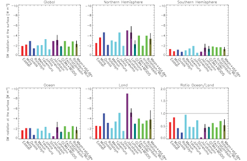
Figure 7.23. Global mean change in net solar radiation at the surface due to the total anthropogenic aerosol effect (direct, semi-direct and indirect cloud albedo and lifetime effects) from pre-industrial times to the present day and its contribution over the NH and SH, over oceans and over land and the ratio over oceans/land. Red bars refer to anthropogenic sulphate ( Easter et al., 2004 [JoC, MoS] ; Ming et al., 2005 [JoC, MoS] +), blue bars to anthropogenic sulphate and organic carbon ( Quaas et al., 2004 [JoC, MoS, SRC] ; Rotstayn and Liu, 2005 [JoC, MoS, SRC] +), turquoise bars to anthropogenic sulphate and black and organic carbon (Menon and del Genio, 2005 [NotFound] ; Takemura et al., 2005 [JoC, MoS, ARC] ; Johns et al., 2006 [JoC, MoS] ; Storelvmo et al., 2006 [JoC, MoS] ), dark purple bars to anthropogenic sulphate and black and organic carbon effects on water and ice clouds ( (Jacobson, 2006; ) Lohmann and Diehl, 2006 [JoC, SRC] ), teal bars refer to a combination of GCM and satellite results (LMDZ/ECHAM plus MODIS, Quaas et al., 2006 [SRC] ), green bars refer to results from coupled atmosphere/mixed-layer ocean (MLO) experiments ( Feichter et al., 2004 [JoC, MoS, SRC] : sulphate and black and organic carbon; Kristjansson et al., 2005 [JoC, MoS] : sulphate and black carbon; Rotstayn and Lohmann, 2002 [JoC, SRC] +:sulphate only) and olive bars to the mean from all simulations. Vertical black lines refer to ±1 standard deviation.
+ refers to estimates solely from the indirect effects
Transient simulations ( Roeckner et al., 1999 [JoC, MoS, SRC] ) and coupled GCM-mixed-layer ocean equilibrium simulations ( Feichter et al., 2004 [JoC, MoS, SRC] ; Liepert et al., 2004 [JoC, SRC] ) suggest that the decrease in solar radiation at the surface resulting from increases in optical depth due to the direct and indirect anthropogenic aerosol effects is more important for controlling the surface energy budget than the greenhouse-gas induced increase in surface temperature. There is a slight increase in downwelling longwave radiation due to aerosols, which in the global mean is small compared to the decrease in shortwave radiation at the surface. The other components of the surface energy budget (thermal radiative flux, sensible and latent heat fluxes) decrease in response to the reduced input of solar radiation. As global mean evaporation must equal precipitation, a reduction in the latent heat flux in the model leads to a reduction in precipitation ( Liepert et al., 2004 [JoC, SRC] ). This is in contrast to the observed precipitation evolution in the last century (see Section 3.3 )and points to an overestimation of aerosol influences on precipitation. The simulated decrease in global mean precipitation from pre-industrial times to the present may reverse into an increase of about 1% in 2031 to 2050 as compared to 1981 to 2000, because the increased warming due to black carbon and greenhouse gases then dominates over the sulphate cooling ( Roeckner et al., 2006 [JoC, ARC] ).
7.5.4 Effects of Aerosols on Circulation Patterns
7.5.4.1 Effects on Stability
Changes in the atmospheric lapse rate modify the longwave emission and affect the water vapour feedback ( Hu, 1996 [JoC] ) and the formation of clouds (see, e.g., Section 8.6 ). Observations and model studies show that an increase in the lapse rate produces an amplification of the water vapour feedback ( Sinha, 1995 [JoC] ). As aerosols cool the Earth’s surface and warm the aerosol layer, the lapse rate will decrease globally and suppress the water vapour feedback (e.g., Feichter et al., 2004 [JoC, MoS, SRC] ). The local change in atmospheric stability strongly depends on the altitude of the black carbon heating ( Penner et al., 2003 [JoC, ARC] ).
Absorption of solar radiation by aerosols can change the cloud amount (semi-direct effect; ( Grassl, 1975; ) Hansen et al., 1997 [JoC, MoS, ARC] ; Ackerman et al., 2000 [JoC] ; Ramanathan et al., 2001 [JoC, ARC] ;( Jacobson, 2006; ) Figure 7.20 ). The semi-direct effect has been simulated with GCMs and high-resolution cloud-resolving models, since it is implicitly accounted for whenever absorbing aerosols coupled to the radiation scheme are included ( Hansen et al., 1997 [JoC, MoS, ARC] ; Lohmann and Feichter, 2001 [JoC, SRC] ; Jacobson, 2002 [JoC] ; Menon et al., 2002b [JoC, SRC] ; Penner et al., 2003 [JoC, ARC] ; Cook and Highwood, 2004 [JoC, MoS] ; Hansen et al., 2005 [JoC, MoS, ARC] ). Aerosol heating within cloud layers reduces cloud fractions, whereas aerosol heating above the cloud layer tends to increase cloud fractions. When diagnosed within a GCM framework, the semi-direct effect can also include cloud changes due to circulation effects and/or surface albedo effects. Moreover, the semi-direct effect is not exclusive to absorbing aerosol, as potentially any radiative heating of the mid-troposphere can produce a similar response in a GCM ( Hansen et al., 2005 [JoC, MoS, ARC] ; see also Section 2.8 ). Cloud-resolving models of cumulus and stratocumulus case studies also diagnose semi-direct effects indicating a similar relationship between the height of the aerosol layer relative to the cloud and the sign of the semi-direct effect ( Ackerman et al., 2000 [JoC] ; Ramanathan et al., 2001 [JoC, ARC] ; Johnson et al., 2004 [JoC] ; Johnson, 2005 [JoC, MoS] ). Using a large eddy simulation, Feingold et al. 2005 [JoC] ) show that the reduction in net surface radiation and in surface latent and sensible heat fluxes is the most simple explanation of the reduction in cloudiness associated with absorbing aerosols.
7.5.4.2 Effects on the Large-Scale Circulation
Several studies have considered the response of a GCM with a mixed-layer ocean to indirect aerosol effects ( Rotstayn et al., 2000 [JoC, SRC] ; K. Williams et al., 2001 [JoC] ; Rotstayn and Lohmann, 2002 [JoC, SRC] ) or to a combination of direct and indirect aerosol effects ( Feichter et al., 2004 [JoC, MoS, SRC] ; Kristjansson et al., 2005 [JoC, MoS] ; Takemura et al., 2005 [JoC, MoS, ARC] ). All of these, and recent transient simulations ( Held et al., 2005 [JoC, MoS, ARC] ; Paeth and Feichter, 2006 [JoC, MoS, SRC] ), found a substantial cooling that was strongest in the NH, with a consequent southward shift of the Inter-Tropical Convergence Zone (ITCZ) and the associated tropical rainfall belt. Rotstayn and Lohmann 2002 [JoC, SRC] ) even suggest that aerosol effects might have contributed to the Sahelian droughts of the 1970 s and 1980 s (see Sections 9.5 and 11.2 ). If in turn the NH is warmed, for instance due to the direct forcing by black carbon aerosols, the ITCZ is found to shift northward ( Chung and Seinfeld, 2005 [JoC, MoS] ).
Menon et al. 2002b [JoC, SRC] and Wang 2004 [Ambiguous] ) found that circulation changes could be caused by aerosols in southeast China. In India and China, where absorbing aerosols have been added, increased rising motions are seen as well as increased subsidence to the south and north ( Menon et al., 2002b [JoC, SRC] ). However, Ramanathan et al. 2005 [JoC, ARC] ) found that convection was suppressed due to increased stability resulting from black carbon heating. Drier conditions resulting from suppressed rainfall can induce more dust and smoke due to the burning of drier vegetation ( Ramanathan et al., 2001 [JoC, ARC] ), thus affecting both regional and global hydrological cycles ( Wang, 2004 [Ambiguous] ). Heating of a lofted dust layer could increase the occurrence of deep convection ( Stephens et al., 2004 [JoC] ). It can also strengthen the Asian summer monsoon circulation and cause a local increase in precipitation, despite the global reduction of evaporation that compensates aerosol radiative heating at the surface ( Miller et al., 2004b [JoC, MoS] ). The dust-induced thermal contrast changes between the Eurasian continent and the surrounding oceans are found to trigger or modulate a rapidly varying or unstable Asian winter monsoon circulation, with a feedback to reduce the dust emission from its sources ( (Zhang et al., 2002 ) ).
In summary, an increase in atmospheric aerosol load decreases air quality and reduces the amount of solar radiation reaching the surface. This negative radiative forcing competes with the greenhouse gas warming for determining the change in evaporation and precipitation. At present, no transient climate simulation accounts for all aerosol-cloud interactions, so that the net aerosol effect on clouds deduced from models is not conclusive.
7.6 Concluding Remarks
Biogeochemical cycles interact closely with the climate system over a variety of temporal and spatial scales. On geological time scales, this interaction is illustrated by the Vostok ice core record, which provides dramatic evidence of the coupling between the carbon cycle and the climate system. The dynamics of the Earth system inferred from this record result from a combination of external forcing (in this case long-term periodic changes in the orbital parameters of the Earth and hence solar forcing) and an array of feedback mechanisms within the Earth environment (see Chapter6 ). On shorter time scales, a range of forcings originating from human activities (conversion and fragmentation of natural ecosystems, emissions of greenhouse gases, nitrogen fixation, degradation of air quality, stratospheric ozone depletion) is expected to produce planet-wide effects and perturb numerous feedback mechanisms that characterise the dynamics of the Earth system.
Anumber of feedbacks that amplify or attenuate the climate response to radiative forcing have been identified. In addition to the well-known positive water vapour and ice-albedo feedbacks, a feedback between the carbon cycle and the climate system could produce substantial effects on climate. The reduction in surface carbon uptake expected in future climate should produce an additional increase in the atmospheric CO2 concentration and therefore enhance climate forcing. Large differences between models, however, make the quantitative estimate of this feedback uncertain. Other feedbacks (involving, for example, atmospheric chemical and aerosol processes) are even less well understood. Their magnitude and even their sign remain uncertain. Potentially important aerosol-cloud interactions such as changes in cloud lifetime and aerosol effects on ice clouds can influence the hydrologic cycle and the radiative budget; however, the scientific understanding of these processes is low. The response of the climate system to anthropogenic forcing is expected to be more complex than simple cause and effect relationships would suggest; rather, it could exhibit chaotic behaviour with cascades of effects across the different scales and with the potential for abrupt and perhaps irreversible transitions.
This chapter has assessed how processes related to vegetation dynamics, carbon exchanges, gas-phase chemistry and aerosol microphysics could affect the climate system. These processes, however, cannot be considered in isolation because of the potential interactions that exist between them. Air quality and climate change, for example, are intimately coupled ( Dentener et al., 2006 [SRC] Brasseur and Roeckner 2005 [JoC, MoS, SRC] ) estimate that the hypothetical removal from the atmosphere of the entire burden of anthropogenic sulphate aerosol particles (in an effort to improve air quality) would produce a rather immediate increase of about 0.8°C in the globally averaged temperature, with geographical patterns that bear a resemblance to the temperature changes found in greenhouse gas scenario experiments( Figure 7.24 ). Thus, environmental strategies aimed at maintaining ‘global warming’ below a prescribed threshold must therefore account not only for CO2 emissions but also for measures implemented to improve air quality. To cope with the complexity of Earth system processes and their interactions, and particularly to evaluate sophisticated models of the Earth system, observations and long-term monitoring of climate and biogeochemical quantities will be essential. Climate models will have to reproduce accurately the important processes and feedback mechanisms discussed in this chapter.
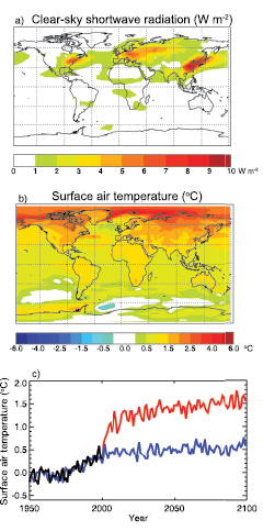
Figure 7.24. Effect of removing the entire burden of sulphate aerosols in the year 2000 on (a) the annual mean clear sky TOA shortwave radiation (Wm–2)calculated by Brasseur and Roeckner 2005 [JoC, MoS, SRC] ) for the time period 2071 to 2100 and (b) on the annual mean surface air temperature (°C) calculated for the same time period. (c) temporal evolution of global and annual mean surface air temperature anomalies (°C) with respect to the mean 1961 to 1990 values. The evolution prior to the year 2000 is driven by observed atmospheric concentrations of greenhouse gases and aerosols as adopted by IPCC (see Chapter 10 ). After 2000, the concentration of greenhouse gases remains constant while the aerosol burden is unchanged (blue line) or set to zero (red line). The black curve shows observations (A. Jones et al., 2001 [Ambiguous] ; Jones et al., 2006 [NPR, PoC, ARC] ).
References
Achard, F., et al., 2004: Improved estimates of net carbon emissions from land cover change in the tropics for the 1990s. Global Biogeochem. Cycles, 18,GB2008, doi:10.1029/2003GB002142. [JoC, MoS]
ACIA, 2005: Arctic Climate Impact Assessment.Cambridge University Press, Cambridge, 1042 pp. [NPR]
Ackerman, A.S., M.P. Kirkpatrick, D.E. Stevens, and O.B. Toon, 2004: The impact of humidity above stratiform clouds on indirect climate forcing. Nature, 432,1014–1017. [JoC, MoS]
Ackerman, A.S., et al., 2000: Reduction of tropical cloudiness by soot. Science, 288,1042–1047. [JoC]
Adams, J., J. Constable, A. Guenther, and P. Zimmerman, 2001: An estimate of natural volatile organic compound emissions from vegetation since the last glacial maximum. Chemosphere, 3,73–91. [MoS, SRC]
Adler, R.F., et al., 2003: The version-2 Global Precipitation Climatology Project (GPCP) monthly precipitation analysis (1979-present). J. Hydrometeorol., 4,1147–1167. [JoC, ARC]
Ainsworth, E.A., and S.P. Long, 2005: What have we learned from 15 years of free-air CO2 enrichment (FACE)? A meta-analytic review of the responses of photosynthesis, canopy. New Phytol., 165(2), 351–371. Clean
Albrecht, B., 1989: Aerosols, cloud microphysics, and fractional cloudiness. Science, 245,1227–1230. [JoC]
Allan, W., et al., 2005: Interannual variations of 13Cin tropospheric methane: Implications for a possible atomic chlorine sink in the marine boundary layer. J. Geophys. Res., 110,doi:10.1029/2004JD005650. [JoC]
Allen, D., K. Pickering, and M. Fox-Rabinovitz, 2004: Evaluation of pollutant outflow and CO sources during TRACE-P using model-calculated, aircraft-based, and Measurements of Pollution in the Troposphere (MOPITT)-derived CO concentrations. J. Geophys. Res., 109,D15S03, doi:10.1029/2003JD004250. [JoC, MoS]
Anderson, T.L., et al., 2003: Climate forcing by aerosols - a hazy picture. Science, 300,1103–1104. [JoC, MoS]
Andreae, M.O., and P. Merlet, 2001: Emission of trace gases and aerosols from biomass burning. Global Biogeochem. Cycles, 15,955–966. [JoC]
Andreae, M.O., C.D. Jones, and P.M. Cox, 2005: Strong present-day aerosol cooling implies a hot future. Nature, 435(7046), 1187–1190. [JoC, MoS, SRC]
Andreae, M.O., et al., 2004: Smoking rain clouds over the Amazon. Science, 303,1337–1342. [JoC]
Angert, A., et al., 2004: CO2 seasonality indicates origins of post-Pinatubo sink. Geophys. Res. Lett., 31(11), L11103, doi:10.1029/2004GL019760. [JoC]
Angert, A., et al., 2005: Drier summers cancel out the CO2 uptake enhancement induced by warmer springs. Proc. Natl. Acad. Sci. U.S.A., 102,10823–10827. [JoC]
Archer, D., 2005: The fate of fossil fuel CO2 in geologic time. J. Geophys. Res., 110(C9), C09S05, doi:10.1029/2004JC002625. [JoC, SRC]
Archer, D., and B. Buffett, 2005: Time-dependent response of the global ocean clathrate reservoir to climatic and anthropogenic forcing. Geochem. Geophys. Geosystems, 6,Q03002, doi:10.1029/2004GC000854. [MoS, SRC]
Archer, D., H. Kheshgi, and E. Maier-Reimer, 1998: Dynamics of fossil fuel CO2 neutralization by marine CaCO3. Global Biogeochem. Cycles, 12(2), 259–276. [JoC, SRC]
Arellano, A.F. Jr., et al., 2004: Top-down estimates of global CO sources using MOPITT measurements. Geophys. Res. Lett., 31,L01104, doi:10.1029/ 2003GL018609. [JoC, MoS]
Armstrong, R.A., et al., 2002: A new, mechanistic model for organic carbon fluxes in the ocean based on the quantitative association of POC with ballast minerals. Deep-Sea Res. II, 49,219–236. [MoS]
Arora, V.K., and G.J. Boer, 2003: A representation of variable root distribution in dynamic vegetation models. Earth Interactions, 7(6), 1–19. [MoS, SRC]
Arora, V.K., and G.J. Boer, 2005: A parameterization of leaf phenology for the terrestrial ecosystem component of climate models. Global Change Biol., 11(1), 39–59. [MoS, SRC]
Arora, V.K., and G.J. Boer, 2006: Simulating competition and coexistence between plant functional types in a dynamic vegetation model. Earth Interactions, 10,Paper 10, 30 pp., doi:10.1175/EI170.1. [MoS, SRC]
Aumont, O., et al., 2001: Riverine-driven interhemispheric transport of carbon. Global Biogeochem. Cycles, 15,393–405. [JoC]
Austin, J., and R.J. Wilson, 2006: Ensemble simulations of the decline and recovery of stratospheric ozone. J. Geophys. Res., 111,D16314, doi:10.1029/2005JD006907. [JoC, MoS, SRC]
Austin, J., et al., 2003: Uncertainties and assessments of chemistry-climate models of the stratosphere. Atmos. Chem. Phys., 3,1–27. [MoS, SRC]
Avissar, R., and D. Werth, 2005: Global hydroclimatological teleconnections resulting from tropical deforestation. J. Hydrometeorol., 6(2), 134–145. [JoC]
Avissar, R., P.L. Silva Dias, M.A.F. Silva Dias, and C. Nobre, 2002: The Large-scale Biosphere-Atmosphere Experiment in Amazonia (LBA): Insights and future research needs. J. Geophys. Res., 107(D20), 8034, doi:10.1029/2002JD002507. [JoC, MoS]
Aw, J., and M.J. Kleeman, 2003: Evaluating the first-order effect of intraannual air pollution on urban air pollution. J. Geophys. Res., 108, 4365, doi:10.1029/2002JD002688. [JoC]
Ayers, G.P., 2005: “Air pollution and climate change: has air pollution suppressed rainfall over Australia?” Clean Air and Environmental Quality, 39,51–57. Clean
Bacastow, R.B., and C.D. Keeling, 1981: Atmospheric carbon dioxide concentration and the observed airborne fraction. In: Carbon Cycle Modelling [Bolin, B. (ed.)]. SCOPE 16. John Wiley and Sons, New York, pp. 103–112. [NPR, MoS, ARC]
Bagnoud, N., A.J. Pitman, B.J. McAvaney, and N.J. Holbrook, 2005: The contribution of the land surface energy balance complexity to differences in means, variances and extremes using the AMIP-II methodology. Clim. Dyn., 25,171–188. doi:10.1007/S00382-005-0004-9. [JoC, SRC]
Baker, D.F., et al., 2006: TransCom 3 inversion intercomparison: impact of transport model errors on the interannual variability of regional CO2 fluxes, 1988-2003. Global Biogeochem. Cycles, 20,GB1002, doi:1010.1029/2004GB002439. [JoC, MoS, SRC]
Baker, M., and R.J. Charlson, 1990: Bistability of CCN concentrations and thermodynamics in the cloud-topped boundary layer. Nature, 345,142–145. [JoC]
Baker, T.R., et al., 2004: Increasing biomass in Amazonian forest plots. Philos. Trans. R. Soc. London Ser.B, 359,353–365. Clean
Baldocchi, D., et al., 2001: FLUXNET: A new tool to study the temporal and spatial variability of ecosystem-scale carbon dioxide, water vapor, and energy flux densities. Bull. Am. Meteorol. Soc., 82,2415–2434. [JoC]
Baldwin, M.P., and T.J. Dunkerton, 1999: Downward propagation of the Arctic Oscillation from the stratosphere to the troposphere. J. Geophys. Res., 104,30937–30946. [JoC, ARC]
Baldwin, M.P., and T.J. Dunkerton, 2001: Stratospheric harbingers of anomalous weather regimes. Science, 244,581–584. [JoC, ARC]
Balkanski, Y., et al., 2004: Global emissions of mineral aerosol: formulation and validation using satellite imagery. In: Emission of Atmospheric Trace Compounds [Granier, C., P. Artaxo, and C.E. Reeves (eds.)]. Kluwer, Dordrecht, pp. 239–267. [NPR]
Balzter H., et al., 2005: Impact of the Arctic Oscillation pattern on interannual forest fire variability in Central Siberia. Geophys. Res. Lett., 32,L14709, doi:10.1029/2005GL022526. [JoC]
Barbosa, P.M., et al., 1999: An assessment of vegetation fire in Africa (1981–1991): Burned areas, burned biomass, and atmospheric emissions. Global Biogeochem. Cycles, 13,933–950. [JoC]
Barford, C.C., et al., 2001: Factors controlling long and short term sequestration of atmospheric CO2 in a mid-latitude forest. Science, 294(5547), 1688–1691. [JoC]
Barlage, M., and X. Zeng, 2004: Impact of observed vegetation root distribution on seasonal global simulations of land surface processes. J. Geophys. Res., 109,D09101, doi:10.1029/2003JD003847. [JoC, MoS]
Battle, M., et al., 2000: Global carbon sinks and their variability inferred from atmosphericO2 and δ13C. Science, 287(5462), 2467–2470. [JoC]
Beirle, S., et al., 2004: Estimate of nitrogen oxide emissions from shipping by satellite remote sensing. Geophys. Res. Lett., 31,L18102, doi:10.1029/2004GL020312. [JoC, MoS]
Bellamy, P.H., et al., 2005: Carbon losses from all soils across England and Wales 1978–2003. Nature, 437,245248. [JoC]
Benner R., et al., 1992: Bulk chemical characteristics of dissolved organic matter in the ocean. Science, 255,1561–1564. [JoC]
Bergamaschi, P., M. Braeunlich, T. Marik, and C.A.M. Brenninkmeijer. 2000: Measurements of the carbon and hydrogen isotopes of atmospheric methane at Izana, Tenerife: Seasonal cycles and synoptic-scale variations. J. Geophys. Res., 105,14531–14546. [JoC]
Berner, R.A., 1998: The carbon cycle and CO2 over Phanerozoic time: the role of land plants. Philos. Trans. R. Soc. London Ser.B, 353(1365), 75–81. Clean
Bertram, T.H., et al., 2005: Satellite measurements of daily variations in soil NOx emissions. Geophys. Res. Lett., 32,L24812, doi:10.1029/2005GL024640. [JoC]
Betts, A.K., 2004: Understanding hydrometeorology using global models. Bull. Am. Meteorol. Soc., 85,1673–1688. [JoC, MoS]
Betts, A.K., 2006: Radiative scaling of the nocturnal boundary layer and the diurnal temperature range. J. Geophys. Res., 111,D07105, doi:10.1029/2005JD006560. [JoC]
Betts, A.K., J. Ball, and J. McCaughey, 2001: Near-surface climate in the boreal forest. J. Geophys. Res., 106,33529–33541. [JoC]
Betts, R., et al., 2004: The role of ecosystem-atmosphere interactions in simulated Amazonian precipitation decrease and forest dieback under global change warming. Theor. Appl. Climatol., 78(1–3), 157–175. [MoS, SRC]
Bey, I., et al., 2001: Global modeling of tropospheric chemistry with assimilated meteorology: model description and evaluation. J. Geophys. Res., 106(D19), 23073–23096. [JoC, MoS]
Bigg, E.K., C. Leck, and L. Tranvik, 2004: Particulates of the surface microlayer of open water in the central Arctic Ocean in summer. Mar. Chem., 91(1–4), 131–141. [SRC]
Bodeker, G.E., H. Shiona, and H. Eskes, 2005: Indicators of Antarctic ozone depletion. Atmos. Chem. Phys., 5,2603–2615. [ARC]
Boersma, K.F., H.J. Eskes, E.W. Meijer, and H.M. Keider, 2005: Estimates of lightning NOx production from GOME satellite observations. Atmos. Chem. Phys. Discussions, 5, 3047–3104. [MoS]
Bogner, J.E., R.L. Sass, and B.P. Walter, 2000: Model comparisons of methane oxidation across a management gradient: Wetlands, rice production systems, and landfill. Global Biogeochem. Cycles., 14,1021–1033. [JoC, MoS]
Bolin, B., and E. Eriksson, 1959: Changes in the carbon dioxide content of the atmosphere and sea due to fossil fuel combustion. In: The Atmosphere and Sea in Motion [Bolin, B. (ed.)]. Rossby Memorial Volume. Rockefeller Institute, New York, NY, pp. 130–142. [NPR]
Bonan, G.B., 2001: Observational evidence for reduction of daily maximum temperature by croplands in the midwest United States. J. Clim., 14,2430–2442. [JoC, SRC]
Bonan, G.B., et al., 2003: A dynamic global vegetation model for use with climate models: concepts and description of simulated vegetation dynamics. Global Change Biol., 9,1543–1566. [MoS, SRC]
Bond, W.J., G.F. Midgley, and F.I. Woodward, 2003: The importance of low atmospheric CO2 and fire in promoting the spread of grasslands and savannas. Global Change Biol., 9,973–982. Clean
Bopp, L., et al., 2002: Climate-induced oceanic oxygen fluxes: Implications for the contemporary carbon budget. Global Biogeochem. Cycles, 16,doi:10.1029/2001GB001445. [NPR, JoC]
Bopp, L., et al., 2004: Will marine dimethyl sulfide emissions amplify or alleviate global warming? A model study. Can. J. Fish Aquat. Sci., 61(5), 826–835. [MoS]
Bopp, L., et al., 2005: Response of diatoms distribution to global warming and potential implications – a global model study. Geophys. Res. Lett., 32(19), L19606, doi:10.1029/2005GL023653. [JoC, MoS]
Borges, A.V., 2005: Do we have enough pieces of the jigsaw to integrate CO2 fluxes in the coastal ocean? Estuaries, 28,3–27. Clean
Bousquet, P., et al., 2000: Regional changes in carbon dioxide fluxes of land and oceans since 1980. Science, 290(5495), 1342–1346. [JoC, SRC]
Bousquet, P., et al., 2005: Two decades of OH variability as inferred by an inversion of atmospheric transport and chemistry of methyl chloroform, Atmos. Chem. Phys., 5,2635–2656. [SRC]
Bouwman, A.F., L.J.M. Boumans, and N.H. Batjes, 2001:Global Estimates of Gaseous Emission of NH3,NO andN2Ofrom Agricultural Land.Food and Agriculture Organisation, Rome, 57 pp. [NPR, MoS]
Bouwman, A.F., L.J.M. Boumans, and N.H. Batjes, 2002: Modeling global annualN2Oand NO emissions from fertilized fields. Global Biogeochem. Cycles, 16(4), 1080, doi:10.1029/2001GB001812. [JoC, MoS]
Boyd, P.W., et al., 2004: The decline and fate of an iron-induced subarctic phytoplankton bloom. Nature, 428,549–553. [JoC]
Boyle, E.D., 1988: The role of vertical chemical fractionation in controlling late quaternary atmospheric carbon dioxide. J. Geophys. Res., 93(C12), 15701–15714. [JoC]
Brasseur, G.P, and E. Roeckner, 2005: Impact of improved air quality on the future evolution of climate. Geophys. Res. Lett., 32,L23704, doi:10.1029/2005GL023902. [JoC, MoS, SRC]
Brasseur, G.P., et al., 1998: Past and future changes in global tropospheric ozone: impact on radiative forcing. Geophys. Res. Lett., 25(20), 3807–3810. [JoC, MoS, SRC]
Brasseur, G.P, et al., 2005: Impact of climate change on the future chemical composition of the global troposphere. J. Clim., 19,3932–3951 [JoC, MoS, SRC]
Breshears, D.D., et al., 2005: Regional vegetation die-off in response to global-change-type drought. Proc. Natl. Acad. Sci. U.S.A., 102(42), 15144–15148. [JoC]
Broecker, W.S., 1991: Keeping global change honest. Global Biogeochem. Cycles, 5,191–195. [JoC]
Broecker, W.S., and T. Takahashi, 1978: Neutralization of fossil fuel CO2 by marine calcium carbonate. In: The Fate of Fossil Fuel CO2 in the Ocean [Andersen, N.R., and A. Malahoff (eds.)]. Plenum Press, New York, NY, pp. 213–248. [NPR]
Broecker, W.S., and T.-H. Peng, 1982: Tracers in the Sea.ELDIGIO Press, New York, NY, 689 pp. [NPR, ARC]
Broecker, W.S., and T.-H. Peng, 1986: Carbon cycle: 1985 – glacial to interglacial changes in the operation of the global carbon cycle. Radiocarbon, 28,309–327. [ARC]
Broerse, A.T.C., et al., 2003: The cause of bright waters in the Bering Sea in winter. Continental Shelf Res., 23,1579–1596. Clean
Brook, E., et al., 2000: On the origin and timing of rapid changes in atmospheric methane during the last glacial period. Global Biogeochem. Cycles, 14,559–572. [JoC]
Brovkin, V., et al., 2004: Role of land cover changes for atmospheric CO2 increase and climate change during the last 150 years. Global Change Biol., 10,1253–1266, doi:10.1111/j.1365-2486.2004.00812. [ARC]
Brown, S., and A.E. Lugo, 1982: The storage and production of organic-matter in tropical forests and their role in the global carbon-cycle. Biotropica, 14(3), 161–187. Clean
Brown, T.J., B.L. Hall, and A.L. Westerling, 2004: The impact of twenty-first century climate change on wildland fire danger in the western United States: an applications perspective. Clim. Change, 62,365–388. [JoC]
Buddemeier, R.W., J.A. Kleypas, and R.B. Aronson, 2004: Coral Reefs and Global Climate Change.Pew Centre on Global Climate Change, Arlington, VA, 44 pp. [NPR]
Buffett, B., and D. Archer, 2004: Global inventory of methane clathrate: sensitivity to changes in the deep ocean. Earth Planet. Sci. Lett., 227,185–199. [SRC]
Burkhardt, S., I. Zondervan, and U. Riebesell, 1999: Effect of CO2 concentration on C:N:P ratio in marine phytoplankton: a species comparison. Limnol. Oceanogr., 44(3), 683–690. [SRC]
Burrows, W.H., et al., 2002: Growth and carbon stock change in eucalypt woodlands in northeast Australia: ecological and greenhouse sink implications. Global Change Biol., 8,769–784. Clean
Butchart, N., and A.A. Scaife, 2001: Removal of chlorofluorocarbons by increased mass exchange between the stratosphere and troposphere in a changing climate. Nature, 410,799–802. [JoC]
Butchart, N., et al., 2006: Simulations of anthropogenic change in the strength of the Brewer–Dobson circulation. Clim. Dyn., 27,doi:10.1007/s00382-006-0162-4. [NPR, JoC, MoS]
Butler, T.M., I. Simmonds, and P.J. Rayner, 2004: Mass balance inverse modeling of methane in the 1990s using a chemistry transport model. Atmos. Chem. Phys., 4,2561–2580. [MoS, SRC]
Cakmur, R.V., et al., 2006: Constraining the magnitude of the global dust cycle by minimizing the difference between a model and observations. J. Geophys. Res., 111,doi:10.1029/2005JD005791 [NPR, JoC, MoS]
Caldeira, K., and M.E. Wickett, 2003: Anthropogenic carbon and ocean pH. Nature, 425(6956), 365–368. [JoC]
Cao, M., K. Gregson, and S. Marshall, 1998: Global methane emission from wetlands and its sensitivity to climate change. Atmos. Environ., 32,3291–3299. Clean
Carpenter, L.J., 2003: Iodine in the marine boundary layer. Chem. Rev., 103, 4953–4962. Clean
Chadwick, O.A., et al., 1999: Changing sources of nutrients during four million years of ecosystem development. Nature, 397(6719), 491. [JoC]
Chagnon, F.J.F., R.L. Bras, and J. Wang, 2004: Climatic shift in patterns of shallow clouds over the Amazon. Geophys. Res. Lett., 31(24), L24212, doi:10.1029/2004GL021188. [JoC]
Chambers, J.Q., and S.E. Trumbore, 1999: An age-old problem. Trends Plant Sci., 4(10), 385–386. Clean
Chambers, J.Q., and W.L. Silver, 2004: Some aspects of ecophysiological and biogeochemical responses of tropical forests to atmospheric change. Philos. Trans. R. Soc. London Ser.B, 359(1443), 463–476. Clean
Chance, K., et al., 2000: Satellite observations of formaldehyde over North America from GOME. Geophys. Res. Lett., 27,3461–3464. [JoC]
Chapin, F.S. III, et al., 2005: Role of land-surface changes in arctic summer warming. Science, 310,657–660. [JoC]
Chapman, S.J., and M. Thurlow, 1996: The influence of climate on CO2 and CH4 emissions from organic soils. J. Agric. For. Meteorol., 79,205–217. Clean
Chappellaz, J.A., I.Y. Fung, and A.M. Thompson, 1993: The atmospheric CH4 increase since the last Glacial Maximum (1) Source estimates. Tellus, 45B,228–241. [JoC, SRC]
Chave, J., et al., 2003: Spatial and temporal variation of biomass in a tropical forest: results from a large census plot in Panama. J. Ecol., 91,240–252. Clean
Chen, C.-T.A., K.-K. Liu, and R. MacDonald, 2003: Continental margin exchanges. In: Ocean Biogeochemistry [Fasham, M.J.R. (ed.)]. Springer-Verlag, Berlin, pp. 53–97. [NPR]
Chen, M., P. Xie, and J.E. Janowiak, 2002: Global land precipitation: a 50-yr monthly analysis based on gauge observations. J. Hydrometeorol., 3,249–266. [JoC]
Chen, Y., and J.E. Penner, 2005: Uncertainty analysis for estimates of the first indirect effect. Atmos. Chem. Phys., 5,2935–2948. [ARC]
Chen, Y-H., and R.G. Prinn, 2005: Atmospheric modeling of high- and low-frequency methane observations: Importance of interannually varying transport. J. Geophys. Res., 110,D10303, doi:10.1029/2004JD005542. [JoC, MoS, ARC]
Chen, Y-H., and R.G. Prinn, 2006: Estimation of atmospheric methane emission between 1996-2001 using a 3-D global chemical transport model. J. Geophys. Res., 111,D10307, doi:10.1029/2005JD006058. [JoC, MoS, ARC]
Christensen, T.R., A. Ekberg, L. Ström, and M. Mastepanov, 2003: Factors controlling large scale variations in methane emission from wetlands. Geophys. Res. Lett., 30,1414, doi:10.1029/2002GL016848. [JoC]
Christensen, T.R., et al., 2004: Thawing sub-arctic permafrost: Effects on vegetation and methane emissions. Geophys. Res. Lett., 31,doi:10.1029/2003GL018680. [NPR, JoC]
Chuang, P.Y., R.M. Duvall, M.M. Shafer, and J.J. Schauer, 2005: The origin of water soluble particulate iron in the Asian atmospheric outflow. Geophys. Res. Lett., 32,doi:10.1029/2004GL021946. [NPR, JoC]
Chung, S.H., and J.H. Seinfeld, 2005: Climate response of direct radiative forcing of anthropogenic black carbon. J. Geophys. Res., 110,D11102, doi:10.1029/2004JD005441. [JoC, MoS]
Ciais, P., et al., 1995: Partitioning of ocean and land uptake of CO2 as inferred by δ13C measurements from the NOAA Climate Monitoring and Diagnostics Laboratory Global Air Sampling Network. J. Geophys. Res., 100(D3), 5051–5070. [JoC, SRC]
Ciais, P., et al., 2005a: The potential for rising CO2 to account for the observed uptake of carbon by tropical, temperate, and boreal forest biomes. In: The Carbon Balance of Forest Biomes [Griffiths, H., and P. G. Jarvis (eds.)]. Taylor and Francis, New York, pp. 109–150. [NPR, SRC]
Ciais, P., et al., 2005b: Europe-wide reduction in primary productivity caused by the heat and drought in 2003. Nature, 437(7058), 529–533. [JoC, SRC]
Clair, T.A., J.M. Ehrman, and K. Higuchi, 1999: Changes in freshwater carbon exports from Canadian terrestrial basins to lakes and estuaries under 2xCO2 atmospheric scenario. Global Biogeochem. Cycles, 13(4), 1091–1097. [JoC]
Clark, D.A., 2002: Are tropical forests an important carbon sink? Reanalysis of the long-term plot data. Ecol. Appl., 12,3–7. [SRC]
Clark, D.A., 2004: Sources or sinks? The responses of tropical forests to current and future climate and atmospheric composition. Philos. Trans. R. Soc. London Ser.B, 359,477–491. [MoS, SRC]
Clark, D.B., C.M. Taylor, and A.J. Thorpe, 2004: Feedback between the land surface and rainfall at convective length scales. J. Hydrometeorol., 5(4), 625–639. [JoC]
Coakley, J.A. Jr., and C.D. Walsh, 2002: Limits to the aerosol indirect radiative forcing derived from observations of ship tracks. J. Atmos. Sci., 59,668–680. [JoC, MoS]
Cochrane, M.A., 2003: Fire science for rainforests. Nature, 421(6926), 913–919. [JoC]
Cohan, D.S., et al., 2002: Impact of atmospheric aerosol light scattering and absorption on terrestrial net primary productivity. Global Biogeochem. Cycles, 16(4), 25–34, 1090, doi:10.1029/2001GB001441. [JoC]
Cole, V., et al., 1996: Agricultural options for mitigation of greenhouse gas emissions. In: Climate Change 1995. Impacts, Adaptations and Mitigation of Climate Change: Scientific-Technical Analyses [Watson, R.T, M.C. Zinyowera, R.H. Moss, and D.J. Dokken (eds)]. Cambridge University Press, Cambridge, United Kingdom and New York, NY, USA, pp 745–771. [NPR]
Collier, J.C., and K.P. Bowman, 2004: Diurnal cycle of tropical precipitation in a general circulation model. J. Geophys. Res., 109,D17105, doi:10.1029/2004JD004818. [JoC, MoS]
Collins, W.J., D.S. Stevenson, C.E. Johnson, and R.G. Derwent, 1999: Role of convection in determining the budget of odd hydrogen in the upper troposphere. J. Geophys. Res., 104(D21), 26927–26942. [JoC, SRC]
Collins, W.J., R.G. Derwent, C.E. Johnson, and D.S. Stevenson, 2002: The oxidation of organic compounds in the troposphere and their global warming potentials. Clim. Change, 52(4), 453–479. [JoC, SRC]
Collins, W.J., et al., 2003: Effect of stratosphere-troposphere exchange on the future tropospheric ozone trend. J. Geophys.Res., 108(D12), 8528, doi:10.1029/2002JD002617. [JoC, MoS]
Conrad, R., 1996: Soil microorganisms as controllers of atmospheric trace gases (H2,CO, CH4,OCS,N2O, and NO). Microbiol. Rev., 60,609–640. Clean
Conrad, R., and W. Seiler, 1981: Decomposition of atmospheric hydrogen by soil-microorganisms and soil enzymes. Soil Biol. Biochem., 13,43–49. Clean
Constable, J.V.H., A.B. Guenther, D.S. Schimel, and R.K. Monson, 1999: Modeling changes in VOC emission in response to climate change in the continental United States. Global Change Biol., 5,791–806. [MoS, SRC]
Cook, J., and E.J. Highwood, 2004: Climate response to tropospheric absorbing aerosols in an intermediate general circulation model. Q. J. R. Meteorol. Soc., 130,175–191. [JoC, MoS]
Cooke, W.F., V. Ramaswamy, and P. Kasibhatla, 2002: A general circulation model study of the global carbonaceous aerosol distribution. J. Geophys. Res., 107,4279, doi:10.1029/2001JD001274. [JoC, MoS, ARC]
Cox, P.M., et al., 2000: Acceleration of global warming due to carbon-cycle feedbacks in a coupled climate model. Nature, 408(6809), doi:10.1038/35041539. [JoC, MoS, SRC]
Cox, P.M., et al., 2004: Amazonian forest dieback under climate-carbon cycle projections for the 21st century. Theor. Appl. Climatol., 78,137–156. [MoS, SRC]
Cramer, W., et al., 2001: Global response of terrestrial ecosystem structure and function to CO2 and climate change: results from six dynamic global vegetation models. Global Change Biol., 7(4), 357–374. [MoS]
Crucifix, M., R.A. Betts, and P.M. Cox, 2005: Vegetation and climate variability: a GCM modeling study. Clim. Dyn., 24,457–467, doi:10.1007/S00382-004-0504-z. [JoC, MoS, SRC]
Cui, Z.Q., K.S. Carslaw, Y. Yin, and S. Davies, 2006: A numerical study of aerosol effects on the dynamics and microphysics of a deep convective cloud in a continental environment. J. Geophys. Res., 111,D05201, doi:10.1029/2005JD005981. [JoC]
Curtis, P.S., et al., 2002: Biometric and eddy-covariance based estimates of annual carbon storage in five eastern North American deciduous forests. Agric. For. Meteorol., 113,3–19. [MoS]
Cziczo, D.J., et al., 2004: Observations of organic species and atmospheric ice formation. Geophys. Res. Lett., 31,doi:10.1029/2004GL019822. [NPR, JoC]
Da Rocha, H.R., et al., 2004: Seasonality of water and heat fluxes over a tropical forest in eastern Amazonia. Ecol. Appl., 14,S114–S126. Clean
Dai, A., and K.E. Trenberth, 2002: Estimates of freshwater discharge from continents: latitudinal and seasonal variations. J. Hydrometeorol., 3,660–687. [PoC, JoC, MoS, SRC]
Dameris, M., et al., 2005: Long-term changes and variability in a transient simulation with a chemistry-climate model employing realistic forcing. Atmos. Chem. Phys., 5,2121–2145. [MoS, SRC]
Dameris, M., et al., 2006: Impact of solar cycle for onset of ozone recovery. Geophys. Res. Lett., 33,L03806, doi:10.1029/2005GL024741. [JoC, SRC]
Dargaville, R.J., et al., 2000: Implications of interannual variability in atmospheric circulation on modeled CO2 concentrations and source estimates. Global Biogeochem. Cycles, 14,931–943. [JoC, MoS]
De Leeuw, G., et al., 2001: Atmospheric input of nitrogen into the North Sea: ANICE project overview. Continental Shelf Res., 21(18–19), 2073–2094. Clean
Decho, A.W., 1990: Microbial exopolymer secretions in ocean environments: their role(s) in food webs and marine processes. Oceanogr. Mar. Biol. Annu. Rev., 28,73–153. Clean
DeFries, R.S., et al., 2002: Carbon emissions from tropical deforestation and regrowth based on satellite observations for the 1980s and 1990s. Proc. Natl. Acad. Sci. U.S.A., 99(22), 14256–14261. [JoC]
Degens, E.T., S. Kempe, and A. Spitzy, 1984: Carbon dioxide: A biogeochemical portrait. In: The Handbook of Environmental Chemistry [Hutzinger, O. (ed.)]. Vol. 1, Part C, Springer-Verlag, Berlin, Heidelberg, pp. 127–215. [NPR]
Del Grosso, S.J., A.R. Mosier, W.J. Parton, and D.S. Ojima, 2005: DAYCENT model analysis of past and contemporary soilN2Oand net greenhouse gas flux for major crops in the USA. Soil Tillage Res., 83(1), 9–24. [MoS]
Del Grosso, S.J., et al., 2000: General CH4 oxidation model and comparison of CH4 oxidation in natural and managed systems. Global Biogeochem. Cycles, 14,999–1019. [JoC, MoS]
DeLucia, E.H., D.J. Moore, and R.J. Norby, 2005: Contrasting responses of forest ecosystems to rising atmospheric CO2:implications for the global C cycle. Global Biogeochem. Cycles, 19,G3006, doi:10.1029/2004GB002346. [JoC]
Dentener, F., et al., 1996: Role of mineral aerosol as a reactive surface in the global troposphere. J. Geophys. Res., 101,22869–22889. [JoC, SRC]
Dentener, F., et al., 2003a: Interannual variability and trend of CH4 lifetime as a measure for OH changes in the 1979–1993 time period. J. Geophys. Res., 108(D15), 4442, doi:10.1029/2002JD002916. [JoC, SRC]
Dentener, F., et al., 2003b: Trends and inter-annual variability of methane emissions derived from 1979–1993 global CTM simulations. Atmos. Chem. Phys., 3,73–88. [MoS, SRC]
Dentener, F., et al., 2005: The impact of air pollutant and methane emission controls on tropospheric ozone and radiative forcing: CTM calculations for the period 1990–2030. Atmos. Chem. Phys., 5,1731–1755. [MoS, SRC]
Dentener, F., et al., 2006: The global atmospheric environment for the next generation. Environ. Sci. Technol., 40(11), 3586–3594. [SRC]
Derwent, R.G., W.J. Collins, C.E. Johnson, and D.S. Stevenson, 2001: Transient behaviour of tropospheric ozone precursors in a global 3-D CTM and their indirect greenhouse effects. Clim. Change, 49(4), 463–487. [JoC, SRC]
Desborough, C.E., 1999: Surface energy balance complexity in GCM land surface models. Clim. Dyn., 15,389–403. [JoC, MoS]
Dickens, G.R., 2001: Modeling the global carbon cycle with gas hydrate capacitor: Significance for the latest Paleocene thermal maximum. In: Natural Gas Hydrates: Occurrence, Distribution, and Detection [Paull, C.K., and W.P. Dillon (eds.)]. Geophysical Monographs Vol. 124, American Geophysical Union, Washington, DC, pp. 19–38. [NPR, MoS]
Dickens, G.R., M.M. Castillo, and J.G.C. Walker, 1997: A blast of gas in the latest Paleocene: Simulating first-order effects of massive dissociation of oceanic methane hydrate. Geology, 25,259–262. [MoS]
Dickinson, R.E., G. Wang, X. Zeng, and Q.-C. Zeng, 2003: How does the partitioning of evapotranspiration and runoff between different processes affect the variability and predictability of soil moisture and precipitation? Adv. Atmos. Sci., 20(3), 475–478. [MoS, SRC]
Dickinson, R.E., et al., 2006: The community land model and its climate statistics as a component of the community climate system model. J. Clim., 19,2302–2324. [JoC, MoS, SRC]
Diehl, K., and S. Wurzler, 2004: Heterogeneous drop freezing in the immersion mode: Model calculations considering soluble and insoluble particles in the drops. J. Atmos. Sci., 61,2063–2072. [JoC, MoS]
Dirmeyer, P.A., 2001: An evaluation of the strength of land-atmosphere coupling. J. Hydrometeorol., 2(4), 329–344. [JoC, ARC]
Dlugokencky, E.J., K.A. Masarie, P.M. Lang, and P.P. Tans, 1998: Continuing decline in the growth rate of the atmospheric methane burden. Nature, 393,447–450. [JoC, SRC]
Dlugokencky, E.J., et al., 2001: Measurements of an anomalous global methane increase during 1998. Geophys. Res. Lett., 28,499–502. [JoC, ARC]
Dlugokencky, E.J., et al., 2003: Atmospheric methane levels off: Temporary pause or a new steady state. Geophys. Res. Lett., 30,doi:10.1029/2003GL018126. [JoC, ARC]
D’Odorico, P., and A. Porporato, 2004: Preferential states in soil moisture and climate dynamics. Proc. Natl. Acad. Sci. U.S.A., 101(24), 8848–8851. [JoC]
Doherty, R.M., D.S. Stevenson, W.J. Collins, and M.G. Sanderson, 2005: Influence of convective transport on tropospheric ozone and its precursors in a chemistry-climate model. Atmos. Chem. Phys., 5,3747–3771. [MoS, SRC]
Doney, S.C., et al., 2004: Evaluating global ocean carbon models: the importance of realistic physics. Global Biogeochem. Cycles, 18(3), GB3017, doi:10.1029/2003GB002150. [JoC, MoS]
Douglass, A.R., M.R. Schoeberl, R.B. Rood, and S. Pawson, 2003: Evaluation of transport in the lower tropical stratosphere in a global chemistry and transport model. J. Geophys. Res., 108(D9), 4259, doi:10.1029/2002JD002696. [JoC, MoS]
Duce, R.A., 1995: Sources, distributions and fluxes of mineral aerosols and their relationship to climate. In: Aerosol Forcing of Climate [Charlson, R.J. and J. Heintzenberg (eds.)]. John Wiley & Sons Ltd., Chichester, New York, pp. 43–72. [NPR, MoS]
Dukes, J.S., et al., 2005: Responses of grassland production to single and multiple global environmental changes. PLoS Biol., 3(10), 1829–1836. Clean
Dunn, A.L, et al., 2007: A long-term record of carbon exchange in a boreal black spruce forest: means, responses to interannual variability, and decadal trends. Global Change Biol., 13,577-590, doi:10.1111/j.1365-2486.2006.01221.x. [2007]
Dupre, B., et al., 2003: Rivers, chemical weathering and Earth’s climate. Comptes Rendus Geoscience, 335(16), 1141–1160. Clean
Durieux, L., L.A.T. Machado, and H. Laurent, 2003: The impact of deforestation on cloud cover over the Amazon arc of deforestation. Remote Sens. Environ., 86(1), 132–140. Clean
Dutay, J.C., et al., 2002: Evaluation of ocean model ventilation with CFC-11: comparison of 13 global ocean models. Ocean Modelling, 4(2), 89–102. [JoC, MoS]
Easter, R.C., et al., 2004: MIRAGE: Model description and evaluation of aerosols and trace gases. J. Geophys. Res., 109,doi:10.1029/2004JD004571. [JoC, MoS]
Edwards, D.P., et al., 2004: Observations of carbon monoxide and aerosols from the Terra satellite: Northern Hemisphere variability. J. Geophys. Res., 109,D24202, doi:10.1029/2004JD004727. [JoC]
Eglinton, T.I., and D.J. Repeta, 2004, Organic matter in the contemporary ocean. In: Treatise on Geochemistry [Holland, H.D., and K.K. Turekian (eds.)]. Volume 6, The Oceans and Marine Geochemistry, Elsevier Pergamon, Amsterdam, pp. 145–180. [NPR]
Ehhalt, D.H., 1999: Gas phase chemistry of the troposphere. In: Global Aspects of Atmospheric Chemistry [Baumgärtl, H., W. Grünbein, and F. Hensel (eds.)]. Dr. Dietrich Steinkopf Verlag, Darmstadt, Germany, pp. 21–110. [NPR]
Ek, M.B., and A.A.M. Holtslag, 2004: Influence of soil moisture on boundary layer cloud development. J. Hydrometeorol., 5,86–99. [JoC, ARC]
Engel, A., et al., 2004: Polysaccharide aggregation as a potential sink of marine dissolved organic carbon. Nature, 428,929–932. [JoC]
Enting, I.G., and J.V. Mansbridge, 1991: Latitudinal distribution of sources and sinks of CO2 - Results of an inversion study. Tellus, 43B,156–170. [JoC]
Enting, I.G., C.M. Trudinger, and R.J. Francey, 1995: A synthesis inversion of the concentration and 13Cof atmospheric CO2. Tellus, 47B,35–52. [JoC]
Etheridge, D.M., L.P. Steel, R.J. Francey, and R.L. Langenfelds, 1998: Atmospheric methane between 1000 A.D. and present: Evidence of anthropogenic emissions and climatic variability. J. Geophys. Res., 103,15979–15993. [JoC, ARC]
Etiope, G., 2004: GEM-Geologic Emission of Methane, the missing source in the atmospheric methane budget. Atmos. Environ., 38,3099–3100. Clean
Etiope, G., and R.W. Klusman, 2002: Geologic emissions of methane to the atmosphere. Chemosphere, 49,777–789. Clean
European Commission, 2003: Ozone-Climate Interactions.Air Pollution Research Report 81, EUR 20623, European Commission, Luxembourg, 143 pp. [NPR]
Eyring, V., et al., 2005: A strategy for process-oriented validation of coupled chemistry-climate models. Bull. Am. Meteorol. Soc., 86,1117–1133. [JoC, MoS, SRC]
Falkowski, P., et al., 2000: The global carbon cycle: A test of our knowledge of Earth as a system. Science, 290(5490), 291–296. [JoC]
Falloon, P., et al., 2006: RothCUK – a dynamic modelling system for estimating changes in soil C at 1km scale in the UK. Soil Use Management, 22,274–288. [MoS]
Fan, S., et al., 1998: A large terrestrial carbon sink in North America implied by atmospheric and oceanic carbon dioxide data and models. Science, 282,442–446. [JoC, MoS]
Fang, J., et al., 2001: Changes in forest biomass carbon storage in China between 1949 and 1998. Science, 292,2320–2322. [JoC]
Farquhar, G.D., S. von Caemmerer, and J.A. Berry, 2001: Models of photosynthesis. Plant Physiol., 125(1), 42–45. [MoS, SRC]
Fearnside, P.M., 2000: Global warming and tropical land-use change: greenhouse gas emissions from biomass burning, decomposition and soils in forest conversion, shifting cultivation and secondary vegetation. Clim. Change, 46,115–158. [JoC]
Feddes, R.A., et al., 2001: Modeling root water uptake in hydrological and climate models. Bull. Am. Meteorol. Soc., 82(12), 2797–2809. [JoC, MoS]
Feely, R.A., R. Wanninkhof, T. Takahashi, and P. Tans, 1999: Influence of El Nino on the equatorial Pacific contribution to atmospheric CO2 accumulation. Nature, 398(6728), 597–601. [JoC, ARC]
Feely, R.A., et al., 2002: Seasonal and interannual variability of CO2 in the equatorial Pacific. Deep-Sea Res. II, 49,2443–2469. [ARC]
Feely, R.A., et al., 2004: Impact of anthropogenic CO2 on the CaCO3 system in the oceans. Science, 305,362–366. [JoC, ARC]
Feichter, J., E. Roeckner, U. Lohmann, and B. Liepert, 2004: Nonlinear aspects of the climate response to greenhouse gas and aerosol forcing. J. Clim., 17(12), 2384–2398. [JoC, MoS, SRC]
Feingold, G., S.M. Kreidenweis, and Y.P. Zhang, 1998: Stratocumulus processing of gases and cloud condensation nuclei - 1. Trajectory ensemble model. J. Geophys. Res., 103(D16), 19527–19542. [JoC, MoS]
Feingold, G., H. Jiang, and J. Y. Harrington, 2005: On smoke suppression of clouds in Amazonia. Geophys. Res. Lett., 32,L02804, doi:10.1029/2004GL021369. [JoC]
Feingold, G., W.R. Cotton, S.M. Kreidenweis, and J.T. Davis, 1999: The impact of giant cloud condensation nuclei on drizzle formation in stratocumulus: Implications for cloud radiative properties. J. Atmos. Sci., 56,4100–4117. [JoC]
Fekete, B.M., C.J. Vorosmarty, and W. Grabs, 2002: High-resolution fields of global runoff combining observed river discharge and simulated water balances. Global Biogeochem. Cycles, 16,doi:10.1029/1999GB001254. [NPR, JoC, MoS]
Felzer, B., et al., 2004: Effects of ozone on net primary production and carbon sequestration in the conterminous United States using a biogeochemistry model. Tellus, 56B,230–248. [JoC, MoS]
Ferek, R.J., et al., 1998: Measurements of ship-induced tracks in clouds off the Washington coast. J. Geophys. Res., 103,23199–23206. [JoC]
Ferretti, D.F., et al., 2005: Unexpected changes to the global methane budget over the past 2000 years. Science, 309,1714–1717. [JoC]
Field, C.B., and M.R. Raupach (eds.), 2004: The Global Carbon Cycle: Integrating Humans, Climate, and the Natural World.SCOPE 62, Island Press, Washington, DC, 526 pp. [NPR, SRC]
Finzi, A.C., et al., 2006: Progressive nitrogen limitation of ecosystem processes under elevated CO2 in a warm-temperate forest. Ecology,87, 15–25. Clean
Findell, K.L., and E.A.B. Eltahir, 2003: Atmospheric controls on soil moisture–boundary layer interactions. Part II: Feedbacks within the continental United States. J. Hydrometeorol., 4,570–583. [JoC]
Fioletov, V.E., et al., 2002: Global and zonal total ozone variations estimated from ground-based and satellite measurements: 1964–2000. J. Geophys. Res., 107(D22), 4647, doi:10.1029/2001JD001350. [JoC, MoS]
Flannigan, M.D., B.J. Stocks, and B.M. Wotton, 2000: Climate change and forest fires. Sci. Total Environ., 262,221–229. Clean
Flückiger, J., et al., 2002: High resolution HoloceneN2Oice core record and its relationship with CH4 and CO2. Global Biogeochem. Cycles, 16,doi: 10.1029/2001GB001417. [NPR, JoC]
Folberth, G., D.A. Hauglustaine, P. Ciais, and J. Lathière, 2005: On the role of atmospheric chemistry in the global CO2 budget. Geophys. Res. Lett., 32,L08801, doi:10.1029/2004GL021812. [JoC, SRC]
Folberth, G.A., D.A. Hauglustaine, J. Lathière, and F. Brocheton, 2006: Interactive chemistry in the Laboratoire de Météorologie Dynamique general circulation model: model description and impact of biogenic hydrocarbons on tropospheric chemistry. Atmos. Chem. Phys., 6,2273–2319. [MoS, SRC]
Foley, J.A., et al., 2003: Green Surprise? How terrestrial ecosystems could affect Earth’s climate. Frontiers Ecol. Environ., 1(1), 38–44. Clean
Frankenberg, C., et al., 2005: Assessing methane emission from global space-borne observation. Science, 308,1010–1014. [JoC]
Frankenberg, C., et al., 2006: Satellite chartography of atmospheric methane from SCIAMACHY on board EMVISAT: Analysis of the years 2003 and 2004. J. Geophys. Res., 111,doi:10.1029/2005JD006235. [NPR, JoC]
Freeman, C., et al., 2004: Export of dissolved organic carbon from peatlands under elevated carbon dioxide levels. Nature, 430,195–198. [JoC]
Freitas, S.R., et al., 2005: Monitoring the transport of biomass burning emissions in South America. Environ. Fluid Mech., 5,135–167. Clean
Frew, R., A. Bowie, P. Croot, and S. Pickmere, 2001: Macronutrient and trace-metal geochemistry of an in situ iron-induced Southern Ocean bloom. Deep-Sea Res. II, 48(11–12), 2467–2481. Clean
Friedlingstein, P., J.-L. Dufresne, P.M. Cox, and P. Rayner, 2003: How positive is the feedback between climate change and the carbon cycle? Tellus, 55B(2), 692–700. [JoC, SRC]
Friedlingstein, P., et al., 2001: Positive feedback between future climate change and the carbon cycle. Geophys. Res. Lett., 28,1543–1546, doi:10.1029/2000GL012015. [JoC, MoS, SRC]
Friedlingstein, P., et al., 2006: Climate-carbon cycle feedback analysis: results from the C4MIP model intercomparison. J. Clim., 19,3337–3353. [JoC, MoS, SRC]
Fu, R., and W. Li, 2004: The influence of the land surface on the transition from dry to wet season in Amazonia. Theor. Appl. Climatol., 78,97–110, doi:10.1007/s00704-004-0046-7. Clean
Fueglistaler, S., and P.H. Haynes, 2005: Control of interannual and longer-term variability of stratospheric water vapor. J. Geophys. Res., 110,D24108, doi:10.1029/2005JD006019. [JoC]
Fung, I., S.C. Doney, K. Lindsay, and J. John, 2005: Evolution of carbon sinks in a changing climate. Proc. Natl. Acad. Sci. U.S.A., 102(32), 11201–11206. [JoC, SRC]
Fusco, A.C., and J.A. Logan, 2003: Analysis of 1970-1995 trends in tropospheric ozone at northern hemisphere midlatitudes with the GEOS-CHEM model. J. Geophys. Res., 108(D15), 4449, doi:10.1029/2002JD002742. [JoC, MoS]
Gabric, A.J., et al., 2004: Modeling estimates of the global emission of dimethylsulfide under enhanced greenhouse conditions. Global Biogeochem. Cycles, 18(2), GB2014, doi:10.1029/2003GB002183. [JoC, MoS]
Galloway, J.N., et al., 2004: Nitrogen cycles: past, present, and future. Biogeochemistry, 70(2), 153–226. [MoS]
Gamon, J.A., et al., 2003. Remote sensing in BOREAS: Lessons learned. Remote Sens. Environ., 89,139–162. Clean
Ganzeveld, L.N., et al., 2002: Global soil-biogenic NOx emissions and the role of canopy processes. J. Geophys. Res., 107(D16), 4298, doi:10.1029/2001JD001289. [JoC]
Gao, Z., et al., 2004: Modeling of surface energy partitioning, surface temperature, and soil wetness in the Tibetan prairie using the Simple Biosphere Model 2 (SiB2). J. Geophys. Res., 109,D06102, doi:10.1029/2003JD004089. [JoC, MoS]
Gattuso, J.-P., D. Allemand, and M. Frankignoulle, 1999: Photosynthesis and calcification at cellular, organismal and community levels in coral reefs: a review on interactions and control by carbonate chemistry. Am. Zool., 39,160–183. Clean
Gedney, N., and P. Cox, 2003: The sensitivity of global climate model simulations to the representation of soil moisture heterogeneity. J. Hydrometeorol., 4,1265–1275. [JoC, MoS, SRC]
Gedney, N., P.M. Cox, and C. Huntingford, 2004: Climate feedback from wetland methane emissions. Geophys. Res. Lett., 31,L20503, doi:10.1029/2004GL020919. [JoC, SRC]
Gérard, J.C., et al., 1999: The interannual change of atmospheric CO2:contribution of subtropical ecosystems. Geophys. Res. Lett., 26,243–246. [JoC]
Gettelman, A., J.R. Holton, and K.H. Rosenlof, 1997: Mass fluxes ofO3,CH4,N2O, and CF2Cl2 in the lower stratosphere calculated from observational data. J. Geophys. Res., 102,19149–19159. [JoC, ARC]
Ghan, S.J., G. Guzman, and H. Abdul-Razzak, 1998: Competition between sea salt and sulphate particles as cloud condensation nuclei. J. Atmos. Sci., 55,3340–3347. [JoC]
Giardina, C.P., and M.G. Ryan, 2000: Evidence that decomposition rates of organic carbon in mineral soil do not vary with temperature. Nature, 404,858–861. [JoC]
Gillett, N.P., and D.W.J. Thompson, 2003: Simulation of recent Southern Hemisphere climate change. Science, 302,273–275. [JoC, MoS, ARC]
Gillett, N.P., A.J. Weaver, F.W. Zwiers, and M.D. Flannigan, 2004: Detecting the effect of climate change on Canadian forest fires. Geophys. Res. Lett., 31(18), L18211, doi:10.1029/2004GL020876. [JoC, ARC]
Ginoux, P., et al., 2001: Sources and distributions of dust aerosols simulated with the GOCART model. J. Geophys. Res., 16,20255–20274. [JoC, MoS]
Givati, A., and D. Rosenfeld, 2004: Quantifying precipitation suppression due to air pollution. J. Appl. Meteorol., 43(7), 1038–1056. [JoC]
Gloor, M., et al., 2003: A first estimate of present and preindustrial air-sea CO2 flux patterns based on ocean interior carbon measurements and models. Geophys. Res. Lett., 30(1), 1010, doi:10.1029/2002GL015594. [JoC, MoS]
Goncalves, L.G.G., E.J. Burke, and W.J. Shuttleworth, 2004: Application of improved ecosystem aerodynamics in regional weather forecasts. Ecol. Appl., 14,S17–S21. [MoS]
Gondwe, M., et al., 2003: Correction to ‘‘The contribution of ocean-leaving DMS to the global atmospheric burdens of DMS, MSA, SO, and NSS SO=’’. Global Biogeochem. Cycles, 17,1106, doi:10.1029/2003GB002153. [JoC]
Gong, S.L., 2003: A parameterization of sea-salt aerosol source function for sub- and super-micron particles. Global Biogeochem. Cycles, 17(4), 1097, doi:10.1029/2003GB002079. [JoC]
Gong, S.L., and L.A. Barrie, 2003: Simulating the impact of sea salt on global nss sulphate aerosols. J. Geophys. Res., 108(D16), 4516, doi:10.1029/2002JD003181. [JoC, MoS]
Goodale, C.L., et al., 2002: Forest carbon sinks in the northern hemisphere. Ecol. Appl., 12(3), 891–899. Clean
Goulden, M.L., et al., 2004: Diel and seasonal patterns of tropical forest CO2 exchange. Ecol. Appl., 14,S42–S54. Clean
Grassl, H., 1975: Albedo reduction and radiative heating of clouds by absorbing aerosol particles. Contrib. Atmos. Phys., 48,199–210. Clean
Green, P.A., et al., 2004: Pre-industrial and contemporary fluxes of nitrogen through rivers: a global assessment based on typology. Biogeochemistry, 68(1), 71–105. Clean
Grenfell, J.L., D.T. Shindell, and V. Grewe, 2003: Sensitivity studies of oxidative changes in the troposphere in 2100 using the GISS GCM. Atmos. Chem. Phys., 3,1267–1283. Clean
Grewe, V., et al., 2001: Future changes of the atmospheric composition and the impact on climate change. Tellus, 53B(2), 103–121. [JoC, MoS]
Gruber, N., and C.D. Keeling, 2001: An improved estimate of the isotopic air-sea disequilibrium of CO2:Implications for the oceanic uptake of anthropogenic CO2. Geophys. Res. Lett., 28,555–558. [JoC, MoS, SRC]
Gruber, N., N. Bates, and C.D. Keeling, 2002: Interannual variability in the North Atlantic Ocean carbon sink. Science, 298(5602), 2374–2378. [JoC, SRC]
Gu, L., et al., 2002: Advantages of diffuse radiation for terrestrial ecosystem productivity. J. Geophys. Res., 107(6), 4050, doi:10.1029/2001JD001242. [JoC]
Gu, L., et al., 2003: Response of a deciduous forest to the Mt. Pinatubo eruption: enhanced photosynthesis. Science, 299(5615), 2035–2038. [JoC]
Guenther, A.B., et al., 1993: Isoprene and monoterpene emission rate variability - model evaluations and sensitivity analyses. J. Geophys. Res., 98(D7), 12609–12617. [JoC, MoS, SRC]
Guenther, A.B., et al., 1995: A global-model of natural volatile organic-compound emissions. J. Geophys. Res., 100(D5), 8873–8892. [JoC, MoS, SRC]
Guenther, A.B., et al., 1999: Isoprene emission estimates and uncertainties for the Central African EXPRESSO study domain. J. Geophys. Res., 104(D23), 30625–30639. [JoC, MoS, SRC]
Guillevic, P., et al., 2002: Influence of the interannual variability of vegetation on the surface energy balance - a global sensitivity study. J. Hydrometeorol., 3,617–629. [JoC]
Guo, Z., et al., 2006. GLACE: The Global Land-Atmosphere Coupling Experiment. 2. Analysis. J. Hydrometeorol., 7,611–625. [JoC]
Gupta, M., et al., 1997: 12C/13Ckinetic isotope effects in the reactions of CH4 with OH and Cl. Geophys. Res. Lett., 24,2761–2764. [JoC]
Gurney, K.R., et al., 2002: Towards robust regional estimates of CO2 sources and sinks using atmospheric transport models. Nature, 415(6872), 626–630. [JoC, MoS, SRC]
Gurney, K.R., et al., 2003: TransCom 3 CO2 inversion intercomparison: 1. Annual mean control results and sensitivity to transport and prior flux information. Tellus, 55B(2), 555–579. [JoC, SRC]
Gurney, K.R., et al., 2004: Transcom 3 inversion intercomparison: model mean results for the estimation of seasonal carbon sources and sinks. Global Biogeochem. Cycles, 18(1), GB1010, doi:10.1029/2003GB002111. [JoC, MoS, SRC]
Gurney, K.R., et al., 2005: Sensitivity of atmospheric CO2 inversions to seasonal and interannual variations in fossil fuel emissions. J. Geophys. Res., 110,D10308, doi:10.1029/2004JD005373. [JoC, SRC]
Haag, W., and B. Kärcher, 2004: The impact of aerosols and gravity waves on cirrus clouds at midlatitudes. J. Geophys. Res., 109,doi:10.1029/2004JD004579. [NPR, JoC, SRC]
Haake, B., and V. Ittekkot, 1990: The wind-driven biological pump and carbon removal in the ocean. Naturwissenschaften, 77(2), 75–79. Clean
Hahmann, A.N., 2003: Representing spatial sub-grid precipitation variability in a GCM. J. Hydrometeorol., 4(5), 891–900. [JoC]
Handisides, G.M., et al., 2003: Hohenpeissenberg photochemical experiment (HOPE 2000): measurements and photostationary state calculations of OH and peroxy radicals. Atmos. Chem. Phys., 3,1565–1588. Clean
Hansell, D.A., and C.A. Carlson, 1998: Deep-ocean gradients in the concentration of dissolved organic carbon. Nature, 395,263–266. [JoC]
Hansen, J., M. Sato, and R. Ruedy, 1997: Radiative forcing and climate response. J. Geophys. Res., 102,6831–6864. [JoC, MoS, ARC]
Hansen, J., et al., 2005: Efficacy of climate forcings. J. Geophys. Res., 110(D18), D18104, doi:10.1029/2005JD005776. [JoC, MoS, ARC]
Hauglustaine, D.A., and G.P. Brasseur, 2001: Evolution of tropospheric ozone under anthropogenic activities and associated radiative forcing of climate. J. Geophys. Res., 106(D23), 32337–32360. [JoC, MoS, SRC]
Hauglustaine, D., and D.H. Ehhalt, 2002: A three-dimensional model of molecular hydrogen in the troposphere. J. Geophys. Res., 107(D17), doi:10.1029/2001JD001156. [JoC, MoS, SRC]
Hauglustaine, D.A., J. Lathière, S. Szopa, and G. Folberth, 2005: Future tropospheric ozone simulated with a climate-chemistry-biosphere model. Geophys. Res. Lett., 32,L24807, doi:10.1029/2005GL024031. [JoC, MoS, SRC]
Hauglustaine, D.A., et al., 2004: Interactive chemistry in the laboratoire de meteorologie dynamique general circulation model: description and background tropospheric chemistry. J. Geophys. Res., 109,D04314, doi:10.1029/2003JD003957. [JoC, MoS, SRC]
Heald, C.L., et al., 2004: Comparative inverse analysis of satellite (MOPITT) and aircraft (TRACE-P) observations to estimate Asian sources of carbon monoxide. J. Geophys. Res., 109(D23), D23306, doi:10.1029/2004JD005185. [JoC, MoS]
Heard, D.E., et al., 2004: High levels of the hydroxyl radical in the winter urban troposphere. Geophys. Res. Lett., 31,L18112, doi:10.1029/2004GL020544. [JoC]
Hein, R., P.J. Crutzen, and M. Heimann, 1997: An inverse modeling approach to investigate the global atmospheric methane cycle. Global Biogeochem. Cycles, 11,43–76. [JoC, MoS, SRC]
Heinze, C., 2004: Simulating oceanic CaCO3 export production in the greenhouse. Geophys. Res. Lett., 31,L16308, doi:10.1029/2004GL020613. [JoC, MoS, SRC]
Heinze, C., E. Maier-Reimer, and K. Winn, 1991: Glacial pCO2 reduction by the World Ocean: experiments with the Hamburg carbon cycle model. Paleoceanography, 6(4), 395–430. [JoC, MoS, SRC]
Heinze, C., et al., 2003: Sensitivity of the marine biospheric Si cycle for biogeochemical parameter variations. Global Biogeochem. Cycles, 17(3), 1086, doi:10.1029/2002GB001943. [JoC, SRC]
Hejzlar, J., M. Dubrovsky, J. Buchtele, and M. Ruzicka, 2003: The apparent and potential effects of climate change on the inferred concentration of dissolved organic matter in a temperate stream (the Malse River, South Bohemia). Sci. Total Environ., 310(1–3), 143–152. Clean
Held, I.M., et al., 2005: Simulation of Sahel drought in the 20th and 21st centuries. Proc. Natl. Acad. Sci. U.S.A., 102(50), 17891–17896 [JoC, MoS, ARC]
Henderson-Sellers, A., P. Irannejad, K. McGuffie, and A.J. Pitman, 2003: Predicting land-surface climates - better skill or moving targets? Geophys. Res. Lett., 30(14), 1777, doi:10.1029/2003GL017387. [JoC, MoS, SRC]
Hendricks, J., B. Kärcher, M. Ponater, and U. Lohmann, 2005: Do aircraft black carbon emissions affect cirrus clouds on a global scale? Geophys. Res. Lett., 32,L12814, doi:10.1029/2005GL022740. [JoC, SRC]
Hendricks, J., et al., 2004: Simulating the global atmospheric black carbon cycle: A revisit to the contribution of aircraft emissions. Atmos. Chem. Phys. 4,2521–2541. [MoS]
Hesselbo, S.P., et al., 2000: Massive dissociation of gas hydrate during a Jurassic oceanic anoxic event. Nature, 406,392–395. [JoC]
Heue, K.-P., et al., 2005: Validation of SCIAMACHY tropospheric NO2 columns with AMAXDOAS measurements. Atmos. Chem. Phys., 5,1039–1051. Clean
Hirsch, A.I., et al., 2006: Inverse modeling estimates of the global nitrous oxide surface flux from 1998–2001. Global Biogeochem. Cycles, 20,GB1008, doi:10.1029/2004GB002443. [JoC, MoS]
Hoerling, M., and A. Kumar, 2003: The perfect ocean for drought. Science, 299(5607), 691–694. [JoC]
Hoffman, W.A., W. Schroeder, and R.B. Jackson, 2002: Positive feedbacks of fire, climate, and vegetation and the conversion of tropical savanna. Geophys. Res. Lett., 15,doi:10.1029/2002G0152. [NPR, JoC]
Hofzumahaus, A., et al., 2004: Photolysis frequency ofO3 to O(1D): Measurements and modeling during the International Photolysis Frequency Measurement and Modeling Intercomparison (IPMMI). J. Geophys. Res., 109,D08S90, doi:10.1029/2003JD004333. [JoC, MoS]
Holland, E.A., and M.A. Carroll, 2003: Atmospheric chemistry and the bio-atmospheric carbon and nitrogen cycles. In: Interactions of the Major Biogeochemical Cycles, Global Change and Human Impacts [Melillo, J.M., C.B. Field, and B. Moldan (eds.)]. SCOPE 61, Island Press, Washington, DC, pp. 273–294. [NPR, SRC]
Holland, E.A., F.J. Dentener, B.H. Braswell, and J.M. Sulzman, 1999: Contemporary and pre-industrial reactive nitrogen budgets. Biogeochemistry, 46,7–43. [SRC]
Holland, E.A., B.H. Braswell, J. Sulzman, and J.F. Lamarque, 2005a: Nitrogen deposition onto the United States and Western Europe: synthesis of observations and models. Ecol. Appl., 15,38–57. [MoS, SRC]
Holland, E.A., J. Lee-Taylor, C. Nevison, and J. Sulzman, 2005b: Global N Cycle: Fluxes andN2Omixing ratios originating from human activity. Data set. Available online from Oak Ridge National Laboratory Distributed Active Archive Center, Oak Ridge, TN, http://www.daac.ornl.gov. [NPR, SRC]
Holland, E.A., et al., 2005c: U.S. nitrogen science plan focuses collaborative efforts. Eos, 86(27), 253–260. [JoC, SRC]
Hollinger, D.Y., et al., 1999: Seasonal patterns and environmental control of carbon dioxide and water vapour exchange in an ecotonal boreal forest. Global Change Biol., 5,891–902. Clean
Holzer, M., and G.J. Boer, 2001: Simulated changes in atmospheric transport climate. J. Clim., 14,4398–4420. [JoC, MoS]
Hong, J., T. Choi, H. Ishikawa, and J. Kim, 2004: Turbulence structures in the near-neutral surface layer on the Tibetan Plateau. Geophys. Res. Lett., 31,L15106, doi:10.1029/2004GL019935. [JoC]
Hoppel, W.A., J.W. Fitzgerald, G.M. Frick, and R.E. Larson, 1990: Aerosol size distributions and optical properties found in the marine boundary layer over the Atlantic Ocean. J. Geophys. Res., 95,3659–3686. [JoC]
Horowitz, L.W., et al., 2003: A global simulation of tropospheric ozone and related tracers: description and evaluation of MOZART, version 2. J. Geophys. Res., 108, 4784, doi:10.1029/2002JD002853. [JoC, MoS]
Houghton, R.A., 1999: The annual net flux of carbon to the atmosphere from changes in land use 1850-1990. Tellus, 51B,298–313. [JoC]
Houghton, R.A., 2003a: Revised estimates of the annual net flux of carbon to the atmosphere from changes in land use and land management 1850-2000. Tellus, 55B(2), 378–390. [JoC, MoS]
Houghton, R.A., 2003b: Why are estimates of the terrestrial carbon balance so different? Global Change Biol., 9,500–509. [MoS]
Houghton, R.A., et al., 2000: Annual fluxes of carbon from deforestation and regrowth in the Brazilian Amazon. Nature, 403,301–304. [JoC]
Houweling, S., F. Dentener, and J. Lelieveld, 1998: The impact of nonmethane hydrocarbon compounds on tropospheric photochemistry. J. Geophys. Res., 103, 10673–10696. [JoC, SRC]
Houweling, S., F. Dentener, and J. Lelieveld, 2000: Simulation of preindustrial atmospheric methane to constrain the global source strength of natural wetlands. J. Geophys. Res., 105,17243–17255. [JoC, MoS, SRC]
Hoyle, C.R., B.P. Luo, and T. Peter, 2005: The origin of high ice crystal number densities in cirrus clouds. J. Atmos. Sci., 62,2568–2579. [JoC]
Hu, H., 1996: Water vapour and temperature lapse rate feedbacks in the mid-latitude seasonal cycle. Geophys. Res. Lett., 23,1761–1764. [JoC]
Huang, Y., R.E. Dickinson, and W.L. Chameides, 2006: Impact of aerosol indirect effect on climate over East Asia. Proc. Natl. Acad. Sci. U.S.A., 103,4371–4376. [JoC, SRC]
Huck, P.E., A.J. McDonald, G.E. Bodeker, and H. Struthers, 2005: Interannual variability in Antarctic ozone depletion controlled by planetary waves and polar temperatures. Geophys. Res. Lett., 32,L13819, doi:10.1029/2005GL022943. [JoC, ARC]
Hudman, R.C., et al., 2004: Ozone production in transpacific Asian pollution plumes and implications for ozone air quality in California. J. Geophys. Res., 109,D23S10, doi:10.1029/2004JD004974. [JoC]
Hughes, T.P., et al., 2003: Climate change, human impacts, and the resilience of coral reefs. Science, 301,929–933. [JoC]
Hungate, B., et al., 2003: Nitrogen and climate change. Science, 302(5650), 1512–1513. [JoC]
Huntingford, C., et al., 2004: Using a GCM analogue model to investigate the potential for Amazonian forest dieback. Theor. Appl. Climatol., 78(1–3), 177–185. [MoS]
Hurst, D.F., et al., 2006: Continuing global significance of emissions of Montreal Protocol-restricted halocarbons in the USA and Canada. J. Geophys. Res., 111,D15302, doi:10.1029/2005JD006785. [JoC]
Hurtt, G.C., et al., 2002: Projecting the future of the U.S. carbon sink. Proc. Natl. Acad. Sci. U.S.A., 99(3), 1389–1394. [JoC, MoS]
IFFN, 2003: Russian Federation Fire 2002 Special. Part III: The 2002 fire season in the Asian part of the Russian Federation: A view from space. International Forest Fire News (IFFN), 28,18–28. [NPR]
Imhoff, M.L., et al., 2004: Global patterns in human consumption of net primary production. Nature, 429(6994), 870–873. [JoC]
IPCC, 2000: Special Report on Emission Scenarios. A Special Report of Working Group III of the Intergovernmental Panel on Climate Change [Nakićenović, N., et al. (eds.)]. Cambridge University Press, Cambridge, United Kingdom and New York, NY, USA, 599 pp. [NPR]
IPCC/TEAP, 2005: IPCC/TEAP Special Report on Safeguarding the Ozone Layer and the Global Climate System: Issues related to Hydrofluorocarbons and Perfluorocarbons. Prepared by Working Group I and III of the Intergovernmental Panel on Climate Change and the Technology and Economic Assessment Panel [Metz, B., et al. (eds.)]. Cambridge University Press, Cambridge, United Kingdom and New York, NY, USA, 488 pp. [NPR]
Irannejad, P., A. Henderson-Sellers, and S. Sharmeen, 2003: Importance of land-surface parameterisation for latent heat simulation in global atmospheric models. Geophys. Res. Lett., 30(17), 1904, doi:10.1029/2003GL018044. [JoC, MoS, SRC]
Irie, H., et al., 2005: Evaluation of long-term tropospheric NO2 data obtained by GOME over East Asia in 1996-2002. Geophys. Res. Lett., 32,L11810, doi:10.1029/2005GL022770. [JoC]
Ishimatsu, A., et al., 2004: Effects of CO2 on marine fish: larvae and adults. J. Oceanogr., 60,731–741. Clean
Ittekkot, V., 1993: The abiotically driven biological pump in the ocean and short-term fluctuations in atmospheric CO2 contents. Global Planet. Change, 8(1–2), 17–25. [JoC]
Jacob, D.J., 2000: Heterogeneous chemistry and tropospheric ozone. Atmos. Environ., 34,2131–2159. [SRC]
Jacob, D.J., et al., 1993: Factors regulating ozone over the United States and its export to the global atmosphere. J. Geophys. Res., 98,14817–14826. [JoC, SRC]
Jacobson, M.Z., 1999: Effects of soil moisture on temperatures, winds, and pollutant concentrations in Los Angeles. J. Appl. Meteorol., 38(5), 607–616. [JoC]
Jacobson, M.Z., 2001: Global direct radiative forcing due to multicomponent anthropogenic and natural aerosols. J. Geophys. Res., 106,1551–1568. [JoC, MoS]
Jacobson, M.Z., 2002: Control of fossil-fuel particulate black carbon and organic matter, possibly the most effective method of slowing global warming. J. Geophys. Res., 107,doi:10.1029/2001JD001376. [JoC]
Jacobson, M.Z., 2006: Effects of externally-through-internally-mixed soot inclusions within clouds and precipitation on global climate. J. Phys. Chem.A, 110,6860–6873. Clean
Jaeglé, L., D.J. Jacob, W.H. Brune, and P.O. Wenberg, 2001: Chemistry of HOx radicals in the upper troposphere. Atmos. Environ., 35,469–489. [SRC]
Jaeglé, L., L. Steinberger, R.V. Martin, and K. Chance, 2005: Global partitioning of NOx sources using satellite observations: Relative roles of fossil fuel combustion, biomass burning and soil emissions. Faraday Discuss., 130,407–423. Clean
Jaeglé, L., et al., 2004: Satellite mapping of rain-induced nitric oxide emissions from soils. J. Geophys. Res., 109,D21310, doi:10.1029/2004JD004787. [JoC]
Jaenicke, R., 2005: Abundance of cellular material and proteins in the atmosphere. Science, 308(5718), doi:10.1126/science.1106335. [JoC]
Jaffe, D., et al., 2004: Long-range transport of Siberian biomass burning emissions and impact on surface ozone in western North America. Geophys. Res. Lett., 31,L16106, doi:10.1029/2004GL020093. [JoC]
Jahren, A.H., et al., 2001: Terrestrial record of methane hydrate dissociation in the Early Cretaceous. Geology, 29(2), 159–162. Clean
Jain, A.K., and X. Yang, 2005: Modeling the effects of two different land cover change data sets on the carbon stocks of plants and soils in concert in CO2 and climate change. Global Biogeochem. Cycles, 19,doi:10.1029/2004GB002349. [NPR, JoC, MoS]
Janssens, I.A., et al., 2003: Europe’s terrestrial biosphere absorbs 7 to 12% of European anthropogenic CO2 emissions. Science, 300(5625), 1538–1542. [JoC]
Jiang, H., et al., 2006: Aerosol effects on the lifetime of shallow cumulus. Geophys. Res. Lett., 33,doi:10.1029/2006GL026024. [NPR, JoC]
Jickells, T.D., et al., 2005: Global iron connections between desert dust, ocean biogeochemistry, and climate. Science, 308(5718), 67–71. [JoC]
Jin, M.L., J.M. Shepherd, and M.D. King, 2005: Urban aerosols and their variations with clouds and rainfall: a case study for New York and Houston. J. Geophys. Res., 110,doi:10.1029/2004JD005081. [JoC, ARC]
Jin, Y., et al., 2002: How does snow impact the albedo of vegetated land surfaces as analyzed with MODIS data? Geophys. Res. Lett., 29,doi:10.1029/2001GLO14132. [NPR, JoC]
Johns, T.C., et al., 2006: The new Hadley Centre climate model HadGEM1: Evaluation of coupled simulations. J. Clim., 19,1327–1353. [JoC, MoS]
Johnson, B.T., 2005: The semidirect aerosol effect: Comparison of a single-column model with large eddy simulation for marine stratocumulus. J. Clim., 18,119–130. [JoC, MoS]
Johnson, B.T., K.P. Shine, and P.M. Forster, 2004: The semi-direct aerosol effect: Impact of absorbing aerosols on marine stratocumulus. Q. J .R. Meteorol. Soc., 130,1407–1422. [JoC]
Johnson, C.E., W.J. Collins, D.S. Stevenson, and R.G. Derwent, 1999: Relative roles of climate and emissions changes on future tropospheric oxidant concentrations. J. Geophys. Res., 104(D15), 18631–18645. [JoC, MoS, SRC]
Johnson, C.E., D.S. Stevenson, W.J. Collins, and R.G. Derwent, 2001: Role of climate feedback on methane and ozone studied with a coupled ocean-atmosphere-chemistry model. Geophys. Res. Lett., 28(9), 1723–1726. [JoC, MoS, SRC]
Johnson, C.E., D.S. Stevenson, W.J. Collins, and R.G. Derwent, 2002: Interannual variability in methane growth rate simulated with a coupled ocean-atmosphere-chemistry model. Geophys. Res. Lett., 29(19), 1903, doi:10.1029/2002GL015269. [JoC, MoS, SRC]
Johnson, D.B., 1982: The role of giant and ultragiant aerosol particles in warm rain initiation. J. Atmos. Sci., 39,448–460. [JoC]
Jones, A., D.L. Roberts, M.J. Woodage, and C. E. Johnson, 2001: Indirect sulphate aerosol forcing in a climate model with an interactive sulphur cycle. J. Geophys. Res., 106,20293–20310. [JoC, MoS, SRC]
Jones, C., N. Mahowald, and C. Luo, 2004: Observational evidence of African desert dust intensification of easterly waves. Geophys. Res. Lett., 31,doi:10.1029/2004GL020107. [NPR, JoC, SRC]
Jones, C.D., and P.M. Cox, 2001a: Modelling the volcanic signal in the atmospheric CO2 record. Global Biogeochem. Cycles, 15(2), 453–466. [JoC, MoS, SRC]
Jones, C.D., and P.M. Cox, 2001b: Constraints on the temperature sensitivity of global soil respiration from the observed interannual variability in atmospheric CO2. Atmos. Sci. Lett., 1,doi:10.1006/asle.2001.0041. [NPR, SRC]
Jones, C.D., and P.M. Cox, 2005: On the significance of atmospheric CO2 growth rate anomalies in 2002–2003. Geophys. Res. Lett., 32,L14816, doi:10.1029/2005GL023027. [JoC, SRC]
Jones, C.D., M. Collins, P.M. Cox, and S.A. Spall, 2001: The carbon cycle response to ENSO: a coupled climate-carbon cycle model study. J. Clim., 14,4113–4129. [JoC, MoS, SRC]
Jones, C.D., et al., 2005: Global climate change and soil carbon stocks: predictions from two contrasting models for the turnover of organic carbon in soil. Global Change Biol., 11(1), 154–166. [MoS, SRC]
Jones, P.D., D.E. Parker, T.J. Osborn, and K.R. Briffa, 2006: Global and hemispheric temperature anomalies--land and marine instrumental records. In: Trends: A Compendium of Data on Global Change. Carbon Dioxide Information Analysis Center, Oak Ridge National Laboratory, U.S. Department of Energy, Oak Ridge, TN. [NPR, PoC, ARC]
Kanakidou, M., et al., 2005: Organic aerosol and global climate modelling: a review. Atmos. Chem. Phys., 5,1053–1123. [MoS]
Kärcher, B., and U. Lohmann, 2002: A parameterization of cirrus cloud formation: homogeneous freezing of supercooled aerosols. J. Geophys. Res., 107,doi:10.1029/2001JD000470. [NPR, JoC, SRC]
Kärcher, B., and U. Lohmann, 2003: A parameterization of cirrus cloud formation: heterogeneous freezing. J. Geophys. Res., 108,doi:10.1029/2002JD003220. [NPR, JoC, SRC]
Kärcher, B., and J. Ström, 2003: The roles of dynamical variability and aerosols in cirrus cloud formation. Atmos. Chem. Phys., 3,823–838. [SRC]
Kärcher, B., and T. Koop, 2004: The role of organic aerosols in homogeneous ice formation. Atmos. Chem. Phys., 4,6719–6745. [SRC]
Kärcher, B., J. Hendricks, and U. Lohmann, 2006: Physically-based parameterization of cirrus cloud formation for use in global atmospheric models. J. Geophys. Res., 111,doi:10.1029/2005JD006219. [NPR, JoC, MoS, SRC]
Karlsdottir, S., and I.S.A. Isaksen, 2000: Changing methane lifetime: Possible cause for reduced growth. Geophys. Res. Lett., 27(1), 93–96. [JoC]
Kasibhatla, P., et al., 2002: Top-down estimate of a large source of atmospheric carbon monoxide associated with fuel combustion in Asia. Geophys. Res. Lett., 29(19), 1900, doi:10.1029/2002GL015581. [JoC, MoS]
Kasischke, E.S., and L.P. Bruhwiler, 2002: Emissions of carbon dioxide, carbon monoxide, and methane from boreal forest fires in 1998. J. Geophys. Res., 107,8146, doi:10.1029/2001JD000461. [JoC]
Kasischke, E.S., N.L. Christensen, and B.J. Stocks, 1995: Fire, global warming and the carbon balance of boreal forests. Ecol. Appl., 5(2), 437–451. Clean
Kasischke, E.S., et al., 2005: Influences of boreal fire emissions on Northern Hemisphere atmospheric carbon and carbon monoxide. Global Biogeochem. Cycles, 19(1), GB1012, doi:10.1029/2004GB002300. [JoC]
Katz, M.E., D.K. Pak, G.R. Dickens, and K.G. Miller. 1999: The source and fate of massive carbon input during the Latest Paleocene Thermal Maximum. Science, 286,1531–1533. [JoC]
Kaufman, Y.J., and I. Koren, 2006: Smoke and pollution aerosol effect on cloud cover. Science, 313,655–658, doi:10.1126/science.1126232. [JoC]
Kaufman, Y.J., et al., 2005: The effect of smoke, dust, and pollution aerosol on shallow cloud development over the Atlantic Ocean. Proc. Natl. Acad. Sci. U.S.A., 102(32), 11207–11212. [JoC]
Kawamiya, M., et al., 2005: Development of an integrated Earth system model on the Earth Simulator. J. Earth Simulator, 4,18–30. [MoS, SRC]
Keeling, C.D., and T.P. Whorf, 2005: Atmospheric CO2 records from sites in the SIO air sampling network. In: Trends: A Compendium of Data on Global Change.Carbon Dioxide Information Analysis Center, Oak Ridge National Laboratory, U.S. Department of Energy, Oak Ridge, TN, http://cdiac.esd.ornl.gov/trends/co2/sio-keel-flask/sio-keel-flask.html. [NPR, ARC]
Keller, M., et al., 2005: Soil-atmosphere exchange for nitrous oxide, nitric oxide, methane, and carbon dioxide in logged and undisturbed forest in the Tapajos National Forest, Brazil. Earth Interactions, 9,1–28, doi:10.1175/EI125.1. Clean
Keppler, F., J.T.G. Hamilton, M. Brass, and T. Roeckmann, 2006: Methane emissions from terrestrial plants under aerobic conditions. Nature, 439,187–191. [JoC]
Kerkweg, A., S. Wurzler, T. Reisin, and A. Bott, 2003: On the cloud processing of aerosol particles: An entraining air-parcel model with two-dimensional spectral cloud microphysics and a new formulation of the collection kernel. Q. J. R. Meteorol. Soc., 129(587), 1–18. [JoC, MoS]
Kettle, A., and M. Andreae, 2000: Flux of the dimethylsulfide from the oceans: A comparison of updated data sets and flux models. J. Geophys. Res., 105,26793–26808. [JoC, MoS]
Key, R.M., et al., 2004: A global ocean carbon climatology: Results from Global Data Analysis Project (GLODAP). Global Biogeochem. Cycles, 18(4), GB4031, doi:10.1029/2004GB002247. [JoC]
Khain, A.P., D. Rosenfeld, and A. Pokrovsky, 2001: Simulating convective clouds with sustained supercooled liquid water down to –37.5°C using a spectral microphysics model. Geophys. Res. Lett., 28,3887–3890. [JoC, MoS]
Khain, A.P., D. Rosenfeld, and A. Pokrovsky, 2005: Aerosol impact on the dynamics and microphysics of convective clouds. Q. J. R. Meteorol. Soc., 131(611), 2639–2663. [JoC]
Khain, A.P., et al., 2004: Simulation of effects of atmospheric aerosols on deep turbulent convective using a spectral microphysics mixed-phase cumulus cloud model. 1. Model description and possible applications. J. Atmos. Sci., 61,2963–2982. [JoC, MoS]
Khalil, M.A.K., and M.J. Shearer, 2006: Decreasing emissions of methane from rice agriculture.Int. Congress Ser., 1293,33–41. Clean
Kirschbaum, M.U.F., et al., 2006: A comment on the quantitative significance of aerobic methane release by plants. Funct. Plant Biol., 33,521–530. Clean
Kirschvink, J.L., and T.D. Raub, 2003: A methane fuse for the Cambrian explosion: carbon cycles and true polar wander. Comptes Rendus Geoscience, 335,65–78. Clean
Klaas, C., and D.E. Archer, 2002: Association of sinking organic matter with various types of mineral ballast in the deep sea: Implications for the rain ratio. Global Biogeochem. Cycles, 16(4), 1116, doi:10.1029/2001GB001765. [JoC]
Kleffmann, J., et al., 2005: Daytime formation of nitrous acid: a major source of OH radicals in a forest. Geophys. Res. Lett., 32,L05818, doi:10.1029/2005GL022524. [JoC]
Kleypas, J.A., J. McManus, and L. Menez, 1999a: Using environmental data to define reef habitat: where do we draw the line? Am. Zool., 39,146–159. Clean
Kleypas, J.A., et al., 1999b: Geochemical consequences of increased atmospheric carbon dioxide on coral reefs. Science, 284,118–120. [JoC]
Kloster, S., et al., 2006: DMS cycle in the marine ocean-atmosphere system - a global model study. Biogeosciences, 3,29–51. [MoS]
Knorr, W., I.C. Prentice, J.I. House, and E.A. Holland, 2005: Long-term sensitivity of soil carbon turnover to warming. Nature, 433,298–301. [JoC, SRC]
Knowlton, K., et al., 2004: Assessing ozone-related health impacts under a changing climate. Environ. Health Perspect., 112,1557–1563. Clean
Koerner, C., 2004: Through enhanced tree dynamics carbon dioxide enrichment may cause tropical forests to lose carbon. Philos. Trans. R. Soc. London Ser.B, 359,493–498. Clean
Koerner, C., et al., 2005: Carbon flux and growth in mature deciduous forest trees exposed to elevated CO2. Science, 309(5739), 1360–1362. [JoC]
Koren, I., Y.J. Kaufman, L.A. Remer, and J.V. Martins, 2004: Measurements of the effect of smoke aerosol on inhibition of cloud formation. Science, 303,1342–1345. [JoC]
Koren, I., et al., 2005: Aerosol invigoration and restructuring of Atlantic convective clouds. Geophys. Res. Lett., 32(14), L14828, doi:10.1029/2005GL023187. [JoC]
Koster, R.D., and M.J. Suarez, 2001: Soil moisture memory in climate models. J. Hydrometeorol., 2(6), 558–570. [JoC, MoS, ARC]
Koster, R.D., and M.J. Suarez, 2004: Suggestions in the observational record of land-atmosphere feedback operating at seasonal time scales. J. Hydrometeorol., 5(3), doi: 10.1175/1525. [JoC, ARC]
Koster, R.D., M.J. Suarez, R.W. Higgins, and H.M. Van den Dool, 2003: Observational evidence that soil moisture variations affect precipitation. Geophys. Res. Lett., 30(5), 1241. doi:10.1029/2002GL016571. [JoC, ARC]
Koster, R.D., et al., 2000: A catchment-based approach to modeling land surface processes in a general circulation model. 1. Model structure. J. Geophys. Res., 105,24809–24822. [JoC, MoS, ARC]
Koster, R.D., et al., 2002: Comparing the degree of land-atmosphere interaction in four atmospheric general circulation models. J. Hydrometeorol., 3(3), 363–375. [JoC, MoS, ARC]
Koster, R.D., et al., 2004: Regions of strong coupling between soil moisture and precipitation. Science, 305,1138–1140. [JoC, ARC]
Koster, R.D., et al., 2006: GLACE: The Global Land-Atmosphere Coupling Experiment. 1. Overview. J. Hydrometeorol., 7,590–610. [JoC, ARC]
Krakauer, N.Y., and J.T. Randerson, 2003: Do volcanic eruptions enhance or diminish net primary production? Evidence from tree rings. Global Biogeochem. Cycles, 17(4), 1118, doi:10.1029/2003GB002076. [JoC]
Kristjánsson, J.E., 2002: Studies of the aerosol indirect effect from sulphate and black carbon aerosols. J. Geophys. Res., 107,doi:10.1029/2001JD000887. [NPR, JoC]
Kristjánsson, J.E., et al., 2005: Response of the climate system to aerosol direct and indirect forcing: Role of cloud feedbacks. J. Geophys. Res., 110,D24206, doi:10.1029/2005JD006299. [JoC, MoS]
Kroeze, C., A. Mosier, and L. Bouwman, 1999: Closing theN2Obudget: A retrospective analysis. Global Biogeochem. Cycles, 13,1–8. [JoC]
Kroeze, C., E. Dumont, and S.P. Seitzinger, 2005: New estimates of global emissions ofN2Ofrom rivers and estuaries. Environ. Sci., 2,159–165. [MoS]
Krüger, O., and H. Grassl, 2004: Albedo reduction by absorbing aerosols over China. Geophys. Res. Lett., 31,doi:10.1029/2003GL019111. [NPR, JoC]
Kulmala, M., et al., 2004: A new feedback mechanism linking forests, aerosols, and climate. Atmos. Chem. Phys., 4,557–562. Clean
Kurz, W.A., and M. Apps, 1999: A 70-years retrospective analysis of carbon fluxes in the Canadian forest sector. Ecol. Appl., 9,526–547. Clean
Kurz, W.A., M.J. Apps, S.J. Beukema, and T. Lekstrum, 1995: 20th-century carbon budget of Canadian forests. Tellus, 47B(1–2), 170–177. [JoC]
Kvenvolden, K.A., and B.W. Rogers, 2005: Gaia’s breath - global methane exhalations. Mar. Petrol. Geol., 22,579–590. Clean
Labrador, L.J., R. von Kuhlmann, and M.G. Lawrence, 2004: Strong sensitivity of the global mean OH concentration and the tropospheric oxidizing efficiency to the source of NOx from lightning. Geophys. Res. Lett., 31,L06102, doi:10.1029/2003GL019229. [JoC]
Lalli, C.M., and R.W. Gilmer, 1989: Pelagic Snails: The Biology of Holoplanktonic Gastropod Mollusks.Stanford University Press, Palo Alto, CA, 259 pp. [NPR]
Lamarque, J.-F., et al., 2005a: Coupled chemistry-climate response to changes in aerosol emissions: global impact on the hydrological cycle and the tropospheric burdens of OH, ozone and NOx. Geophys. Res. Lett., 32,L16809, doi:10.1029/2005GL023419. [JoC]
Lamarque J.-F., et al., 2005b: Assessing future nitrogen deposition and carbon cycle feedback using a multimodel approach: Part 1. Analysis of nitrogen deposition. J. Geophys. Res., 110,D19303, doi:10.1029/2005JD005825. [JoC, MoS]
Lamarque, J.-F., et al., 2005c: Tropospheric ozone evolution between 1890 and 1990. J. Geophys. Res., 110,D08304, doi:10.1029/2004JD005537. [JoC]
Langdon, C., et al., 2003: Effect of elevated CO2 on the community metabolism of an experimental coral reef. Global Biogeochem. Cycles, 17,1011, doi:10.1029/2002GB001941. [JoC]
Langenbuch, H., and H.O. Pörtner, 2003: Energy budget of heptocytes from Antarctic fish(Pachycara brachycephalum and Lepidonotothen kempi)as a function of ambient CO2:pH-dependent limitations of cellular protein biosynthesis? J. Exp. Biol., 206,3895–3903. Clean
Langenfelds, R.L., et al., 1999: Partitioning of the global fossil CO2 sink using a 19-year trend in atmosphericO2. Geophys. Res. Lett., 26,1897–1900. [JoC]
Langenfelds, R.L., et al., 2002: Interannual growth rate variations of atmospheric CO2 and its 13C,H2,CH4,and CO between 1992 and 1999 linked to biomass burning. Global Biogeochem. Cycles, 16(3), 1048, doi:10.1029/2001GB001466. [JoC]
Langner, J., R. Bergstrom, and V. Foltescu, 2005: Impact of climate change on surface ozone and deposition of sulphur and nitrogen in Europe. Atmos. Environ., 39,1129–1141. Clean
Larsen, S.H., 2005: Solar variability, dimethyl sulphide, clouds, and climate. Global Biogeochem. Cycles, 19,GB1014, doi:10.1029/2004GB002333. [JoC]
Lassey, K.R., D.C Lowe, and M.R. Manning, 2000: The trend in atmospheric methane δ13Cand implications for isotopic constraints on the global methane budget. Global Biogeochem. Cycles, 14,41–49. [JoC, SRC]
Lathière, J., et al., 2005: Past and future changes in biogenic volatile organic compound emissions simulated with a global dynamic vegetation model. Geophys. Res. Lett., 32,L20818, doi:10.1029/2005GL024164. [JoC, MoS]
Laurance, W.F., et al., 2004: Pervasive alteration of tree communities in undisturbed Amazonian forests. Nature, 428,171–175. [JoC]
Lawrence, D.M., and J.M. Slingo, 2004: An annual cycle of vegetation in a GCM. Part I: implementation and impact on evaporation. Clim. Dyn., 22,doi:10.1007/s0038200303669. [NPR, JoC, ARC]
Lawrence, D.M., and J.M. Slingo, 2005: Weak land-atmosphere coupling strength in HadAM3: The role of soil moisture variability. J. Hydrometeorol., 6(5), 670–680, doi:10.1775/JHM445.1. [JoC, ARC]
Lawrence, M.G., R. von Kuhlmann, M. Salzmann, and P.J. Rasch, 2003: The balance of effects of deep convective mixing on tropospheric ozone. Geophys. Res. Lett., 30(18), 1940, doi:10.1029/2003GL017644. [JoC]
Laws, E.A., et al., 2000: Temperature effects on export production in the open ocean. Global Biogeochem. Cycles, 14,1231–1246. [JoC]
Le Quéré, C., et al., 2000: Interannual variability of the oceanic sink of CO2 from 1979 to 1997. Global Biogeochem. Cycles, 14,1247–1265. [JoC, SRC]
Le Quéré, C., et al., 2003: Two decades of ocean CO2 sink and variability. Tellus, 55B(2), 649–656. [JoC, SRC]
Le Quéré, C., et al., 2005: Ecosystem dynamics based on plankton functional types for global ocean biogeochemistry models. Global Change Biol., 11,doi:10.1111/j.1365-2486.2005.001004.x. [NPR, MoS, SRC]
Leck, C., and E.K. Bigg, 2005a: Biogenic particles in the surface microlayer and overlaying atmosphere in the central Arctic Ocean during summer. Tellus, 57B(4), 305–316. [JoC, SRC]
Leck, C., and E.K. Bigg, 2005b: Source and evolution of the marine aerosol - A new perspective. Geophys. Res. Lett., 32,L19803, doi:10.1029/2005GL023651. [JoC, SRC]
Lee, K., et al., 1998: Low interannual variability in recent oceanic uptake of atmospheric carbon dioxide. Nature, 396,155–159. [JoC]
Lefèvre, N., et al., 1999: Assessing the seasonality of the oceanic sink for CO2 in the northern hemisphere. Glob. Biogeochem. Cycles, 13,273–286. [JoC, ARC]
Lelieveld, J., and F.J. Dentener, 2000: What controls tropospheric ozone? J. Geophys. Res., 105, 3531–3551. [JoC, SRC]
Lelieveld, J., W. Peters, F.J. Dentener, and M.C. Krol, 2002a: Stability of tropospheric hydroxyl chemistry. J. Geophys. Res., 107(D23), 4715, doi:10.1029/2002JD002272. [JoC, SRC]
Lelieveld, J., et al., 2002b: Global air pollution crossroads over the Mediterranean. Science, 298,794–799. [JoC]
Leue, C., et al., 2001: Quantitative analysis of NOx emissions from GOME satellite image sequences. J. Geophys. Res., 106,5493–5505. [JoC]
Levin, Z., E. Ganor, and V. Gladstein, 1996: The effects of desert particles coated with sulfate on rain formation in the eastern Mediterranean. J. Appl. Meteorol., 35,1511–1523. [JoC]
Levis, S., and G.B. Bonan, 2004: Simulating springtime temperature patterns in the community atmosphere model coupled to the community land model using prognostic leaf area. J. Clim., 17,4531–4540. [JoC, MoS, SRC]
Levis, S., G.B. Bonan, and C. Bonfils, 2004: Soil feedback drives the mid-Holocene North African monsoon northward in fully coupled CCSM2 simulations with a dynamic vegetation model. Clim. Dyn., 23,doi:10.1007/s00382-004-0477-y. [JoC, MoS, SRC]
Lewis, E.R., and S.E. Schwartz, 2005: Sea Salt Aerosol Production: Mechanisms, Methods, Measurements, and Models: A Critical Review.Geophysical Monograph Vol. 152, American Geophysical Union, Washington, DC, 413 pp. [NPR, MoS, SRC]
Lewis, S.L., Y. Malhi, and O.L. Phillips, 2005: Fingerprinting the impacts of global change on tropical forests. Philos. Trans. R. Soc. London Ser.B, 359,doi:10.1098/rstb.2003.1432. [NPR, SRC]
Li, C., et al., 2002: Reduced methane emissions from large-scale changes in water management of China’s rice paddies during 1980-2000. Geophys. Res. Lett., 29,doi: 10.1029/2002GL015370. [NPR, JoC]
Li, Q., et al., 2005: North American pollution outflow and the trapping of convectively lifted pollution by upper-level anticyclone. J. Geophys. Res., 110,D10301, doi:10.1029/2004JD005039. [JoC]
Li, W., and R. Fu, 2004: Transition of the large-scale atmospheric and land surface conditions from the dry to the wet season over Amazonia as diagnosed by the ECMWF re-analysis. J. Clim., 17,2637–2651. [JoC]
Liang X., Z. Xie, and M. Huang, 2003: A new parameterization for surface and groundwater interactions and its impact on water budgets with the variable infiltration capacity (VIC) land surface model. J. Geophys. Res., 108,8613, doi:19.1029/2002JD003090. [JoC, MoS]
Liao, H., and J.H. Seinfeld, 2005: Global impacts of gas-phase chemistry-aerosol interactions on direct radiative forcing by anthropogenic aerosols and ozone. J. Geophys. Res., 110,D18208, doi:10.1029/2005JD005907. [JoC, MoS]
Liebmann, B., and J.A. Marengo, 2001: Interannual variability of the rainy season and rainfall in the Brazilian Amazon basin. J. Clim., 14(22), 4308–4318. [JoC]
Liepert, B.G., and I. Tegen, 2002: Multidecadal solar radiation trends in the United States and Germany and direct tropospheric aerosol forcing. J. Geophys. Res., 107,doi:10.1029/2001JD000760. [NPR, JoC, MoS, ARC]
Liepert, B.G., J. Feichter, U. Lohmann, and E. Roeckner, 2004: Can aerosols spin down the water cycle in a warmer and moister world. Geophys. Res. Lett., 31,L06207, doi:10.1029/2003GL019060. [JoC, SRC]
Lin, C.-Y.C., D.J. Jacob, and A.M. Fiore, 2001: Trends in exceedances of the ozone air quality standard in the continental United States, 1980-1998. Atmos. Environ., 35, 3217–3228. [SRC]
Lin, G.H., et al., 1999: Ecosystem carbon exchange in two terrestrial ecosystem mesocosms under changing atmospheric CO2 concentrations. Oecologia, 119(1), 97–108. Clean
Lintner, B.R., 2002: Characterizing global CO2 interannual variability with empirical orthogonal function/principal component (EOF/PC) analysis. Geophys. Res. Lett., 29(19), 1921, doi:10.1029/2001GL014419. [JoC]
Liu, X., and J.E. Penner, 2005: Ice nucleation parameterization for a global model. Meteorol. Z., 14(4), 499–514. [MoS, ARC]
Liu, Y., and P.H. Daum, 2002: Indirect warming effect from dispersion forcing. Nature, 419,580–581. [JoC, MoS]
Loh, A.N., J.E. Bauer, and E.R.M. Druffel, 2004: Variable ageing and storage of dissolved organic components in the open ocean. Nature, 430,877–881. [JoC]
Lohmann, U., 2002: A glaciation indirect aerosol effect caused by soot aerosols. Geophys. Res. Lett., 29,doi:10.1029/2001GL014357. [NPR, JoC, SRC]
Lohmann, U., and J. Feichter, 2001: Can the direct and semi-direct aerosol effect compete with the indirect effect on a global scale? Geophys. Res. Lett., 28(1), 159–161, doi:10.1029/2000GL012051. [JoC, SRC]
Lohmann, U., and B. Kärcher, 2002: First interactive simulations of cirrus clouds formed by homogeneous freezing in the ECHAM GCM. J. Geophys. Res., 107,doi:10.1029/2001JD000767. [NPR, JoC, MoS, SRC]
Lohmann, U., and G. Lesins, 2002: Stronger constraints on the anthropogenic indirect aerosol effect. Science, 298,1012–1016. [JoC, SRC]
Lohmann, U., and J. Feichter, 2005: Global indirect aerosol effects: a review. Atmos. Chem. Phys., 5,715–737. [SRC]
Lohmann, U., and K. Diehl, 2006: Sensitivity studies of the importance of dust ice nuclei for the indirect aerosol effect on stratiform mixed-phase clouds. J. Atmos. Sci., 63,1338–1347. [JoC, SRC]
Lohmann, U., I. Koren, and Y.J. Kaufman, 2006: Disentangling the role of microphysical and dynamical effects in determining cloud properties over the Atlantic. Geophys. Res. Lett., 33, L09802, doi:10.1029/2005GL024625. [JoC, SRC]
Lovins, A.B., 2003: Hydrogen primer. RMI Solutions Newsletter, 19(2), 1–4; 36–39. [NPR]
Lucht, W., et al., 2002: Climatic control of the high-latitude vegetation greening trend and Pinatubo effect. Science, 296(5573), 1687–1689. [JoC]
Luo, Y., S.Q. Wan, D.F. Hui, and L.L. Wallace, 2001: Acclimatization of soil respiration to warming in a tall grass prairie. Nature, 413,622–625. [JoC, ARC]
Luo, Y., et al., 2004: Progressive nitrogen limitation of ecosystem responses to rising atmospheric carbon dioxide. Bioscience, 54,731–739. [ARC]
Mack, F., J. Hoffstadt, G. Esser, and J.G. Goldammer, 1996: Modeling the influence of vegetation fires on the global carbon cycle. In: Biomass Burning and Global Change [Levine, J.S. (ed)]. MIT Press, Cambridge, MA, pp. 149–159. [NPR, MoS]
Mahaffey, C., A.F. Michaels, and D.G. Capone, 2005: The conundrum of marineN2 fixation. Am. J. Sci., 305(6–8): 546–595. Clean
Mahowald, N.M., and L.M. Kiehl, 2003: Mineral aerosol and cloud interactions. Geophys. Res. Lett., 30,doi:10.1029/2002GL016762. [NPR, JoC]
Mahowald, N.M., and C. Luo, 2003: A less dusty future? Geophys. Res. Lett., 30(7), 1903, doi:10.1029/2003GL017880. [JoC, MoS]
Mahowald, N.M., G.D.R. Rivera, and C. Luo, 2004: Comment on “Relative importance of climate and land use in determining present and future global soil dust emission” by I. Tegen et al. Geophys. Res. Lett., 31(24), L24105, doi:10.1029/2004GL021272. [JoC, MoS]
Maier-Reimer, E., U. Mikolajewicz, and A.Winguth, 1996: Future ocean uptake of CO2:interaction between ocean circulation and biology. Clim. Dyn., 12,711–721. [JoC, MoS]
Malhi, Y., and J. Grace, 2000: Tropical forests and atmospheric carbon dioxide. Trends Ecol. Evol., 15(8), 332–337. [SRC]
Malhi, Y., and O.L. Phillips, 2004: Tropical forests and global atmospheric change: a synthesis. Philos. Trans. R. Soc. London Ser.B, 359,doi:10.1098/rstb.2003.1449. [NPR, SRC]
Malhi, Y., and J. Wright, 2004: Spatial patterns and recent trends in the climate of tropical rainforest regions. Philos. Trans. R. Soc. London Ser.B, 359,doi:10.1098/rstb.2003.1433. [NPR, SRC]
Malhi, Y., et al., 2002: An international network to understand the biomass and dynamics of Amazonian forests (RAINFOR). J. Veg. Sci., 13,439–450. [SRC]
Manning, A.C., and R.F. Keeling, 2006: Global oceanic and land biotic carbon sinks from the Scripps atmospheric oxygen flask sampling network. Tellus, 58B(2), 95–116. [JoC, ARC]
Marani, M., E. Eltahir, and A. Rinaldo, 2001: Geomorphic controls on regional base flow. Water Resour. Res., 37,2619–2630. Clean
Marengo, J., and C.A. Nobre, 2001: The hydroclimatological framework in Amazonia. In: Biogeochemistry of the Amazon Basin [McClaine, M., R. Victoria, and J. Richey (eds.)]. Oxford University Press, Oxford, UK, pp. 17–42. [NPR]
Marland, G., T.A. Boden, and R.J. Andres, 2006: Global, regional, and national CO2 emissions. In: Trends: A Compendium of Data on Global Change.Carbon Dioxide Information Analysis Center, Oak Ridge National Laboratory, U.S. Department of Energy, Oak Ridge, TN, http://cdiac.esd.ornl.gov/trends/emis/tre_glob.htm. [NPR]
Martin, R.V., et al., 2002: Interpretation of TOMS observations of tropical tropospheric ozone with a global model and in-situ observations. J. Geophys. Res., 107(D18), 4351, doi:10.1029/2001JD001480. [JoC, MoS]
Martin, R.V., et al., 2003a: Global inventory of nitrogen oxide emissions constrained by space-based observations of NO2 columns. J. Geophys. Res., 108(D17), 4537, doi:10.1029/2003JD003453. [JoC]
Martin, R.V., et al., 2003b: Global and regional decreases in tropospheric oxidants from photochemical effects of aerosols. J. Geophys. Res., 108(D3), 4097, doi:10.1029/2002JD002622. [JoC]
Martinerie, P., G.P. Brasseur, and C. Granier, 1995: The chemical composition of ancient atmospheres: a model study constrained by ice core data. J. Geophys. Res., 100,14291–14304. [JoC, MoS, SRC]
Matsumi, Y., et al., 2002: Quantum yields for production of O(1D) in the ultraviolet photolysis of ozone: Recommendation based on evaluation of laboratory data. J. Geophys. Res., 104(D3), doi:10.1029/2001JD000510. [JoC]
Matthews, H.D., M. Eby, A.J. Weaver, and B.J. Hawkins, 2005: Primary productivity control of simulated carbon cycle-climate feedbacks. Geophys. Res. Lett., 32,L14708, doi:10.1029/2005GL022941. [JoC, MoS, ARC]
Matthews, R., and R. Wassmann, 2003: Modelling the impacts of climate change and methane emission reductions on rice production: a review. Eur. J. Agron., 19,573–598. [MoS]
Maynard, K., and J.-F. Royer, 2004: Sensitivity of a general circulation model to land surface parameters in African tropical deforestation experiments. Clim. Dyn., 22,doi:10.1007/s0038200403989. [NPR, JoC, MoS]
McCabe, G.J., M.P. Clark, and M.C. Serreze, 2001: Trends in northern hemisphere surface cyclone frequency and intensity. J. Clim., 14,2763–2768. [JoC]
McFiggans, G., 2005: Marine aerosols and iodine emissions. Nature, 433,E13. [JoC, SRC]
McFiggans, G., et al., 2004: Direct evidence for coastal iodine particles from Laminaria macroalgae - linkage to emissions of molecular iodine. Atmos. Chem. Phys., 4,701–713. [SRC]
McGuire, A.D. III, et al., 2001: Carbon balance of the terrestrial biosphere in the twentieth century: Analyses of CO2,climate and land use effects with four process-based ecosystem models. Global Biogeochem. Cycles, 15,183–206. [JoC, MoS]
McKenzie, R.L., B.J. Connor, and G.E. Bodeker, 1999: Increased summertime UV observed in New Zealand in response to ozone loss. Science, 285,1709–1711. [JoC, ARC]
McKinley, G.A., M.J. Follows, and J. Marshall, 2004a: Mechanisms of air-sea CO2 flux variability in the equatorial Pacific and the North Atlantic. Global Biogeochem. Cycles, 18,GB2011, doi:10.1029/2003GB002179. [JoC]
McKinley, G.A., et al., 2004b: Pacific dominance to global air-sea CO2 flux variability: A novel atmospheric inversion agrees with ocean models. Geophys. Res. Lett., 31,L22308, doi:10.1029/2004GL021069. [JoC, MoS]
McLinden, C., et al., 2000: Stratospheric ozone in 3-D models: a simple chemistry and the cross-tropopause flux. J. Geophys. Res., 105,14653–14665. [JoC, MoS]
McNeil, B.I., et al., 2003: Anthropogenic CO2 uptake by the ocean based on the global chlorofluorocarbon data set. Science, 299(5604), 235–239. [JoC]
Melillo, J.M., et al., 1995: Vegetation/ecosystem modeling and analysis project: Comparing biogeography and biogeochemistry models in a continental-scale study of terrestrial ecosystem responses to climate change and CO2 doubling. Global Biogeochem. Cycles, 9,407–437. [JoC, MoS]
Melillo, J.M., et al., 2002: Soil warming and carbon-cycle feedbacks to the climate system. Science, 298,2173–2176. [JoC]
Menon, S., and A. Del Genio, 2007: Evaluating the impacts of carbonaceous aerosols on clouds and climate. In: An Interdisciplinary Assessment: Human-Induced Climate Change [Schlesinger, M., et al. (eds.)]. Cambridge University Press, Cambridge, UK, in press. [NPR, SRC, 2007]
Menon, S., and L. Rotstayn, 2006: The radiative influence of aerosol effects on liquid-phase cumulus and stratiform clouds based on sensitivity studies with two climate models. Clim. Dyn., 27,345–356. [JoC, MoS, SRC]
Menon, S., A.D. Del Genio, D. Koch, and G. Tselioudis, 2002a: GCM Simulations of the aerosol indirect effect: sensitivity to cloud parameterization and aerosol burden. J. Atmos. Sci., 59,692–713. [JoC, MoS, SRC]
Menon, S., J. Hansen, L. Nazarenko, and Y. Luo, 2002b: Climate effects of black carbon aerosols in China and India. Science, 297,2250–2252. [JoC, SRC]
Menon, S., et al., 2003: Evaluating aerosol/cloud/radiation process parameterizations with single-column models and Second Aerosol Characterization Experiment (ACE-2) cloudy column observations. J. Geophys. Res., 108,doi:10.1029/2003JD003902. [JoC, MoS, SRC]
Mickley, L.J., D.J. Jacob, and D. Rind, 2001: Uncertainty in preindustrial abundance of tropospheric ozone: implications for radiative forcing calculations. J. Geophys. Res., 106,3389–3399. [JoC, MoS, SRC]
Mickley, L.J., D.J. Jacob, B.D. Field, and D. Rind, 2004: Effects of future climate change on regional air pollution episodes in the United States. Geophys. Res. Lett., 30,1862, doi:10.1029/2003GL017933. [JoC, MoS, SRC]
Mickley, L.J., et al., 1999: Radiative forcing from tropospheric ozone calculated with a unified chemistry–climate model. J. Geophys. Res., 104(D23), 30153–30172. [JoC, MoS]
Mikaloff Fletcher, S.E., et al., 2004a: CH4 sources estimated from atmospheric observations of CH4 and its 13C/12Cisotopic ratios: 1. Inverse modeling of source processes. Global Biogeochem. Cycles, 18,GB4004, doi:10.1029/2004GB002223. [JoC, MoS]
Mikaloff Fletcher, S.E., et al., 2004b: CH4 sources estimated from atmospheric observations of CH4 and its 13C/12Cisotopic ratios: 2. Inverse modeling of CH4 fluxes from geographical regions. Global Biogeochem. Cycles, 18,doi:10.1029/2004GB002224. [NPR, JoC, MoS]
Mikaloff Fletcher, S.E., et al., 2006: Inverse estimates of anthropogenic CO2 uptake, transport, and storage by the ocean. Global Biogeochem. Cycles, 18,doi:10.1029/2005GB002530. [NPR, JoC, MoS]
Miller, R.L., J. Perlwitz, and I. Tegen, 2004a: Feedback upon dust emission by dust radiative forcing through the planetary boundary layer. J. Geophys. Res., 109,D24209, doi:10.1029/2004JD004912. [JoC, MoS]
Miller, R.L., I. Tegen, and J. Perlwitz, 2004b: Surface radiative forcing by soil dust aerosols and the hydrologic cycle. J. Geophys. Res., 109,D04203, doi:10.1029/2003JD004085. [JoC, MoS]
Millero, F.J., et al., 2002: Dissociation constants for carbonic acid determined from field measurements. Deep-Sea Res.I, 49,1705–1723. Clean
Milly, P.C.D, and A.B. Schmakin, 2002: Global modeling of land water and energy balances, Part I: The Land Dynamics (LaD) model. J. Hydrometeorol., 3,301–310. [JoC, MoS]
Ming, Y., et al., 2005: Geophysical Fluid Dynamics Laboratory general circulation model investigation of the indirect radiative effects of anthropogenic sulfate aerosol. J. Geophys. Res., 110,D22206, doi:10.1029/2005JD006161. [JoC, MoS]
Montzka, S.A., et al., 1999: Present and future trends in the atmospheric burden of ozone depleting halogens. Nature, 398,690–694. [JoC, MoS, ARC]
Montzka, S.A., et al., 2003: A decline in tropospheric bromine. Geophys. Res. Lett., 30(15), 1826, doi:10.1029/2003GL017745. [JoC, ARC]
Mosier, A., et al., 1998: Closing the globalN2Obudget:N2Oemissions through the agricultural nitrogen cycle-OECD/IPCC.IEA phase II development of IPCC guidelines for national greenhouse gas inventory methodology. Nutrient Cycling in Agroecosystems, 52,225–248. Clean
Mouillot, F., and C.B. Field, 2005: Fire history and the global carbon budget: a 1° x 1° fire history reconstruction for the 20th century. Global Change Biol., 11,398–420. Clean
Müller, J., and G. Brasseur, 1999: Sources of upper tropospheric HOx:A three-dimensional study. J. Geophys. Res., 104(D1), 1705–1716. [JoC, SRC]
Myhre, G., M.M. Kvalevag, and C.B. Schaaf, 2005: Radiative forcing due to anthropogenic vegetation change based on MODIS surface albedo data. Geophys. Res. Lett., 32,L21410, doi: 10.1029/2005GLO24004. [JoC, MoS, ARC]
Nabuurs, G.J., et al., 2003: Temporal evolution of the European forest sector carbon sink from 1950 to 1999. Global Change Biol., 9,152–160. Clean
Nadelhoffer, K., et al., 2004: Decadal-scale fates of N-15 tracers added to oak and pine stands under ambient and elevated N inputs at the Harvard Forest (USA). For. Ecol. Manage., 196,89–107. Clean
Naja, M., H. Akimoto, and J. Staehelin, 2003: Ozone in background and photochemically aged air over central Europe: analysis of long-term ozonesonde data from Hohenpeissenberg and Payerne. J. Geophys. Res., 108(D2), 4063, doi:10.1029/2002JD002477. [JoC]
Naqvi, S.W.A., et al., 2000: Increased marine production ofN2Odue to intensifying anoxia on the Indian continental shelf. Nature, 408(6810), 346–349. [JoC]
Negri, A.J., R.F. Adler, L.M. Xu, and J. Surratt, 2004: The impact of Amazonian deforestation on dry season rainfall. J. Clim., 17(6), 1306–1319. [JoC, ARC]
Neill, C., et al., 2005: Rates and controls of nitrous oxide and nitric oxide emissions following conversion of forest to pasture in Rondônia. Nutrient Cycling in Agroecosystems, 71,1–15. Clean
Nemani, R., et al., 2002: Recent trends in hydrologic balance have enhanced the terrestrial carbon sink in the United States. Geophys. Res. Lett., 29(10), 1468, doi:10.1029/2002GL014867. [JoC]
Nemani, R.R., et al., 2003: Climate-driven increases in global terrestrial net primary production from 1982 to 1999. Science, 300,1560–1563. [JoC]
Nepstad, D., et al., 2004: Amazon drought and its implications for forest flammability and tree growth: a basin-wide analysis. Global Change Biol., 10(5), 704–717. Clean
Nesbitt, S.W., R.Y. Zhang, and R.E. Orville, 2000: Seasonal and global NOxproduction by lightning estimated from the Optical Transient Detector (OTD). Tellus, 52B,1206–1215. [JoC, MoS]
Nevison, C.D., J.H. Butler, and J.W. Elkins, 2003: Global distribution ofN2Oand theN2O/AOU yield in the subsurface ocean. Global Biogeochem. Cycles, 17(4), 1119, doi:10.1029/2003GB002068. [JoC, ARC]
Nevison, C.D., T. Lueker, and R.F. Weiss, 2004: Quantifying the nitrous oxide source from coastal upwelling. Global Biogeochem. Cycles, 18,GB1018, doi:10.1029/2003GB002110. [JoC, ARC]
Newchurch, M.J., et al., 2003: Evidence for slowdown in stratospheric ozone loss: first stage of ozone recovery. J. Geophys. Res., 108(D16), 4507, doi:10.1029/2003jd003471. [JoC]
Newman, P.A., S.R. Kawa, and E.R. Nash, 2004: On the size of the Antarctic ozone hole. Geophys. Res. Lett., 31,L21104, doi:10.1029/2004GL020596. [JoC]
Newman, P.A., et al., 2006: When will the Antarctic ozone hole recover? Geophys. Res. Lett., 33,L12814, doi:10.1029/2005GL025232. [JoC]
Nightingale, P.D., et al., 2000: In situ evaluation of air-sea gas exchange parameterisations using novel conservative and volatile tracers. Global Biogeochem. Cycles, 14(1), 373–387. [JoC]
Nilsson, S., et al., 2003: The missing “missing sink”. Forestry Chronicle, 79(6), 1071–1074. Clean
Niu, G.-Y., and Z.-L. Yang, 2004: Effects of vegetation canopy processes on snow surface energy and mass balances. J. Geophys. Res., 109,D23111, doi:10.1029/2004JD004884. [JoC]
Niyogi, D., et al., 2004: Direct observations of the effects of aerosol loading on net ecosystem CO2 exchanges over different landscapes. Geophys. Res. Lett., 31,L20506, doi:10.1029/2004GL020915. [JoC]
Nober, F.J., H.-F. Graf, and D. Rosenfeld, 2003: Sensitivity of the global circulation to the suppression of precipitation by anthropogenic aerosols. Global Planet. Change, 37,57–80. [JoC]
Norby, R.J., and C.M. Iversen, 2006: Nitrogen uptake, distribution, turnover, and efficiency of use in a CO2-enriched sweetgum forest. Ecology, 87,5–14. Clean
Norton, W.A., 2003: Sensitivity of northern hemisphere surface climate to simulation of the stratospheric polar vortex. Geophys. Res. Lett., 30(12), doi:10.1029/2003GL016958. [JoC, MoS]
Novelli, P.C., et al., 1999: Molecular hydrogen in the troposphere: global distribution and budget. J. Geophys. Res., 104(D23), 30427–30444. [JoC]
Nowak, R.S., D.S. Ellsworth, and S.D. Smith, 2004: Functional responses of plants to elevated atmospheric CO2 – do photosynthetic and productivity data from FACE experiments support early predictions? New Phytol., 162,253–280. [MoS]
NRC (National Research Council), 1991: Rethinking the Ozone Problem in Urban and Regional Air Pollution.National Academy Press, Washington, DC, 524 pp. [NPR]
Obata, A., and Y. Kitamura, 2003: Interannual variability of the sea-air exchange of CO2 from 1961 to 1998 simulated with a global ocean circulation-biogeochemistry model. J. Geophys. Res., 108,3337, doi:10.1029/2001JC001088. [JoC, MoS]
O’Dowd, C.D., 2002: On the spatial extent and evolution of coastal aerosol plumes. J. Geophys. Res., 107(D19), 8105, doi:10.1029/2001JD000422. [JoC]
O’Dowd, C.D., J.A. Lowe, and M.H. Smith, 1999: Coupling sea-salt and sulphate interactions and its impact on cloud droplet concentration predictions. Geophys. Res. Lett., 26,1311–1314. [JoC, MoS, ARC]
O’Dowd, C.D., et al., 2002a: Coastal new particle formation: Environmental conditions and aerosol physicochemical characteristics during nucleation bursts. J. Geophys. Res., 107(D19), 8107, doi:10.1029/2000JD000206. [JoC]
O’Dowd, C.D., et al., 2002b: A dedicated study of New Particle Formation and Fate in the Coastal Environment (PARFORCE): Overview of objectives and achievements. J. Geophys. Res., 107(D19), 8108, doi:10.1029/2001JD000555. [JoC]
O’Dowd, C.D., et al., 2004: Biogenically driven organic contribution to marine aerosols. Nature, 431,676–680. [JoC]
Oechel, W.C, et al., 2000: Acclimation of ecosystem CO2 exchange in the Alaskan Arctic in response to decadal climate warming. Nature, 406,978–981. [JoC]
Ogawa, K., and T. Schmugge, 2004: Mapping surface broadband emissivity of the Sahara desert using ASTER and MODIS data. Earth Interactions, 8(7), 1–14. Clean
Ogle, S.M., M.D. Eve, F.J. Breidt, and K. Paustian, 2003: Uncertainty in estimating land use and management impacts on soil organic carbon storage for US agroecosystems between 1982 and 1997. Global Change Biol., 9,1521–1542. [MoS]
Oglesby, R.J., et al., 2002: Thresholds in atmosphere-soil moisture interactions: results from climate model studies. J. Geophys. Res., 107(14), doi:10.1029/2001JD001045. [JoC, MoS]
Okin, G.S., N. Mahowald, O.A. Chadwick, and P. Artaxo, 2004: Impact of desert dust on the biogeochemistry of phosphorus in terrestrial ecosystems. Global Biogeochem. Cycles, 18,GB2005, doi:10.1029/2003GB002145. [JoC, ARC]
Oleson, K.W., G.B. Bonan, S. Levis, and M. Vertenstein, 2004: Effects of land use change on North American climate: impact of surface datasets and model biogeophysics. Clim. Dyn., 23,117–132, doi:10.1007/s00382-004-0426-9. [JoC, MoS, SRC]
Oleson, K.W., et al., 2003: Assessment of global climate model land surface albedo using MODIS data. Geophys. Res. Lett., 30(8), 1443, doi:10.1029/2002GL016749. [JoC, MoS]
Olivié, D.J.L., P.F.J. van Velthoven, A.C.M. Beliaars, and H.M. Kelder, 2004: Comparison between archived and off-line diagnosed convective mass fluxes in the chemistry transport model TM3. J. Geophys. Res., 109,D11303, doi:10.1029/2003JD004036. [JoC, MoS]
Olivier, J.G.J., A.F. Bouwman, K.W. Van Der Hoek, and J.J.M. Berdowski, 1998: Global air emission inventories for anthropogenic sources of NOx,NH3 andN2Oin 1990. Environ. Pollut., 102(1, S1), 135–148. Clean
Olivier, J.G.J., et al., 2005: Recent trends in global greenhouse emissions: regional trends 1970–2000 and spatial distribution of key sources in 2000. Environ. Sci., 2,81–99. Clean
Ollinger, S.V., and J.D. Aber, 2002: The interactive effects of land use, carbon dioxide, ozone, and N deposition. Global Change Biol., 8,545–562 Clean
Olsen, S.C., C.A. McLinden, and M.J. Prather, 2001: StratosphericN2O-NOy system: testing uncertainties in a three-dimensional framework. J. Geophys. Res., 106,28771–28784. [JoC, ARC]
Ordóñez, C., et al., 2005: Changes of daily surface ozone maxima in Switzerland in all seasons from 1992 to 2002 and discussion of summer 2003. Atmos. Chem. Phys., 5,1187–1203. Clean
Oren, R., et al., 2001: Soil fertility limits carbon sequestration by forest ecosystems in a CO2-enriched atmosphere. Nature, 411(6836), 469–472. [JoC]
Orr, J.C., et al., 2001: Estimates of anthropogenic carbon uptake from four three-dimensional global ocean models. Global Biogeochem. Cycles, 15(1), 43–60, doi:10.1029/1999GB001256. [JoC, MoS, ARC]
Orr, J.C., et al., 2005: Anthropogenic ocean acidification over the twenty-first century and its impact on calcifying organisms. Nature, 437(7059), 681–686. [JoC, ARC]
Osborne, T.M., et al., 2004: Influence of vegetation on the local climate and hydrology in the tropics: sensitivity to soil parameters. Clim. Dyn., 23,45–61. [JoC]
Oyama, M.D., and C.A. Nobre, 2004: Climatic consequences of a large-scale desertification in northeast Brazil: a GCM simulation study. J. Clim., 17(16), 3203–3213. [JoC, MoS]
Pacala, S.W., et al., 2001: Consistent land- and atmosphere-based US carbon sink estimates. Science, 292,2316–2320. [JoC, MoS]
Paeth, H., and J. Feichter, 2006: Greenhouse-gas versus aerosol forcing and African climate response. Clim Dyn., 26(1), 35–54. [JoC, MoS, SRC]
Page, S., et al., 2002: The amount of carbon released from peat and forest fires in Indonesia during 1997. Nature, 320,61–65. [JoC]
Pahlow, M., and U. Riebesell, 2000, Temporal trends in deep ocean Redfield ratios. Science, 287,831–833. [JoC, SRC]
Palmer, P.I., et al., 2003a: Inverting for emissions of carbon monoxide from Asia using aircraft observations over the western Pacific. J. Geophys. Res., 108(D21), 8828, doi:10.1029/2003JD003397. [JoC]
Palmer, P.I., et al., 2003b: Mapping isoprene emissions over North America using formaldehyde column observations from space. J. Geophys. Res., 108,4180, doi:10.1029/2002JD002153. [JoC]
Park, R.J., et al., 2004: Global simulation of tropospheric ozone using the University of Maryland Chemical Transport Model (UMD-CTM): 1. Model description and evaluation. J. Geophys. Res., 109,D09301, doi:10.1029/2003JD004266. [JoC, MoS]
Patra, P.K., et al., 2005: Role of biomass burning and climate anomalies for land-atmosphere carbon fluxes based on inverse modeling of atmospheric CO2. Global Biogeochem. Cycles, 19,GB3005, doi:10.1029/2004GB002258 . [JoC, MoS]
Paull, C.K., et al., 2003: An experiment demonstrating that marine slumping is a mechanism to transfer methane from seafloor gas-hydrate deposits into the upper ocean and atmosphere. Geo.-Marine Lett., 22,198–203. Clean
Peng, Y., and U. Lohmann, 2003: Sensitivity study of the spectral dispersion of the cloud droplet size distribution on the indirect aerosol effect. Geophys. Res. Lett., 30(10), 1507, doi:10.1029/2003GL017192. [JoC, SRC]
Peng, Y., et al., 2002: The cloud albedo-cloud droplet effective radius relationship for clean and polluted clouds from ACE and FIRE. J. Geophys. Res., 107(D11), doi:10.1029/2002JD000281. [JoC]
Penner, J., et al., 2001: Aerosols, their direct and indirect effects. In: Climate Change 2001: The Scientific Basis. Contribution of Working Group I to the Third Assessment Report of the Intergovernmental Panel on Climate Change [Houghton, J.T., et al. (eds.)]. Cambridge University Press, Cambridge, United Kingdom and New York, NY, USA, pp. 289–348. [NPR, ARC]
Penner, J.E., S.Y. Zhang, and C.C. Chuang, 2003: Soot and smoke aerosol may not warm climate. J. Geophys. Res., 108(21), 4657, doi:10.1029/2003JD003409. [JoC, ARC]
Penner., J.E., et al., 2006: Model intercomparison of indirect aerosol effects. Atmos. Chem. Phys. Discuss., 6,1579–1617. [MoS, ARC]
Perlwitz, J., I. Tegen, and R.L. Miller, 2001: Interactive soil dust aerosol model in the GISS GCM 1. Sensitivity of the soil dust cycle to radiative properties of soil dust aerosols. J. Geophys. Res., 106(D16), doi:10.1029/2000JD900668. [JoC, MoS]
Perry, K.D., S.S. Cliff, and M.P. Jimenez-Cruz, 2004: Evidence for hygroscopic mineral dust particles from the Intercontinental Transport and Chemical Transformation Experiment. J. Geophys. Res., 109, D23S28, doi:10.1029/2004JD004979. [JoC]
Petit, J., et al., 1999: Climate and atmospheric history of the past 420,000 years from the Vostok ice core, Antarctica. Nature, 399,429–436. [JoC]
Pétron, G., et al., 2004: Monthly CO surface sources inventory based on the 2000-2001 MOPITT data. Geophys. Res. Lett., 31, L21107, doi:10.1029/2004GL020560. [JoC]
Peylin, P., et al., 2005: Multiple constraints on regional CO2 flux variations over land and oceans. Global Biogeochem. Cycles, 19,GB1011, doi:10.1029/2003GB002214. [JoC, SRC]
Phillips, O.L., et al., 1998: Changes in the carbon balance of tropical forests: evidence from long-term plots. Science, 282(5388), 439–442. [JoC]
Phillips, V.T.J., T.W. Choularton, A.M. Blyth, and J. Latham, 2002: The influence of aerosol concentrations on the glaciation and precipitation of a cumulus cloud. Q. J. R. Meteorol. Soc., 128(581), 951–971. [JoC]
Pickering, K.E., et al., 2001: Trace gas transport and scavenging in PEM-Tropics B South Pacific convergence zone convection. J. Geophys. Res., 106(D23), doi:10.1029/2001JD000328. [JoC]
Pielke, R.A. Sr., 2001: Influence of the spatial distribution of vegetation and soils on the prediction of cumulus convective rainfall. Rev. Geophys., 39(2), 151–177. [JoC, MoS]
Pielke, R.A. Sr., and T. Matsui, 2005: Should light wind and windy nights have the same temperature trends at individual levels even if the boundary layer averaged heat content change is the same? Geophys. Res. Lett., 32,L21813, doi:10.1029/2005GL024407. [JoC]
Pinto, J.P., and M.A.K. Khalil, 1991: The stability of tropospheric OH during ice ages, inter-glacial epochs and modern times. Tellus, 43B,347–352. [JoC]
Pinty, B., et al., 2006: Simplifying the interaction of land surfaces with radiation for relating remote sensing products to climate models. J. Geophys. Res., 111,D02116, doi:10.1029/2005JD005952. [JoC, MoS]
Pitman, A.J., B.J. McAvaney, N. Bagnound, and B. Chemint, 2004: Are inter-model differences in AMIP-II near surface air temperature means and extremes explained by land surface energy balance complexity. Geophys. Res. Lett., 31,L05205, doi:10.1029/2003GL019233. [JoC, MoS, SRC]
Platnick, S., et al., 2000: The role of background cloud microphysics in the radiative formation of ship tracks. J. Atmos. Sci., 57,2607–2624. [JoC]
Platt, U., W. Allan, and D. Lowe. 2004: Hemispheric average Cl atom concentration from 12C/13Cratios in atmospheric methane. Atmos. Chem. Phys., 4,2393–2399. [ARC]
Plattner, G.-K., F. Joos, T.F. Stocker, and O. Marchal, 2001: Feedback mechanisms and sensitivities of ocean carbon uptake under global warming. Tellus, 53B,564–592. [PoC, JoC, ARC]
Polvani, L.M. and P.J. Kushner, 2002: Tropospheric response to stratospheric perturbations in a relatively simple general circulation model. Geophys. Res. Lett., 29,doi:10.1029/2001GL014284. [NPR, JoC, MoS, ARC]
Prather, M.J., 2002: Lifetimes of atmospheric species: integrating environmental impacts. Geophys. Res. Lett., 29(22), 2063, doi:10.1029/2002GL016299 [JoC, ARC]
Prather, M.J., et al., 2001: Atmospheric chemistry and greenhouse gases. In: Climate Change 2001: The Scientific Basis. Contribution of Working Group I to the Third Assessment Report of the Intergovernmental Panel on Climate Change [Houghton, J.T., et al. (eds.)]. Cambridge University Press, Cambridge, United Kingdom and New York, NY, USA, pp. 239–287. [NPR, ARC]
Prentice, I.C., et al., 2001: The Carbon Cycle and Atmospheric Carbon Dioxide. In: Climate Change 2001: The Scientific Basis. Contribution of Working Group I to the Third Assessment Report of the Intergovernmental Panel on Climate Change [Houghton, J.T., et al. (eds.)]. Cambridge University Press, Cambridge, United Kingdom and New York, NY, USA, pp. 99–181. [NPR]
Price, C., and D. Rind, 1994a: Possible implications of global climate change on global lightning distributions and frequencies. J. Geophys. Res., 99(D5), doi:10.1029/94JD00019. [JoC, ARC]
Price, C., and D. Rind, 1994b: The impact of a 2xCO2 climate on lightning-caused fires. J. Clim., 7,1484–1494. [JoC, ARC]
Price, C., J. Penner, and M. Prather, 1997: NOxfrom lightning 1. Global distribution based on lightning physics. J. Geophys. Res., 102(D5), doi:10.1029/96JD03504. [JoC, ARC]
Prinn, R.G., et al., 1990: Atmospheric emissions and trends of nitrous-oxide deduced from 10 years of ALE-gauge data. J. Geophys. Res., 95(D11), 18369–18385. [JoC, ARC]
Prinn, R.G., et al., 2001: Evidence for substantial variations of atmospheric hydroxyl radicals in the past two decades. Science, 292(5523), 1882–1888. [JoC, ARC]
Prinn, R.G., et al., 2005: Evidence for variability of atmospheric hydroxyl radicals over the past quarter century. Geophys.Res.Lett., 32,L07809, doi:10.1029/2004GL022228. [JoC, ARC]
Prospero, J.M., and P.J. Lamb, 2003: African droughts and dust transport to the Caribbean: Climate change implications. Science, 302,1024–1027. [JoC]
Prospero, J.M., et al., 2002: Environmental characterization of global sources of atmospheric soil dust identified with the NIMBUS 7 total ozone mapping spectrometer (TOMS) absorbing aerosol product. Rev. Geophys., 40,doi:10.1029/2000RG000095. [JoC]
Qian, Y., and F. Giorgi, 2000: Regional climatic effects of anthropogenic aerosols? The case of Southwestern China. Geophys. Res. Lett., 27(21), doi:10.1029/2000GL011942. [JoC, ARC]
Quaas, J., O. Boucher, and F.-M. Bréon, 2004: Aerosol indirect effects in POLDER satellite data and the Laboratoire de Météorologie Dynamique-Zoom (LMDZ) general circulation model. J. Geophys. Res., 109,doi:10.1029/2003JD004317. [JoC, MoS, SRC]
Quaas, J., O. Boucher, and U. Lohmann, 2006: Constraining the total aerosol indirect effect in the LMDZ and ECHAM4 GCMs using MODIS satellite data. Atmos. Chem. Phys., 6,947-955. [SRC]
Quay, P., et al., 2003: Changes in the 13C/12C of dissolved inorganic carbon in the ocean as a tracer of anthropogenic CO2 uptake. Global Biogeochem. Cycles, 17(1), 1004, doi:10.1029/2001GB001817. [JoC]
Quesada, C.A., et al., 2004: Seasonal and depth variation of soil moisture in a burned open savanna (campo sujo) in central Brazil. Ecol. Appl., 14,S33–41. Clean
Raich, J., and W. Schlesinger, 1992: The global carbon dioxide flux in soil respiration and its relationship to vegetation and climate. Tellus, 44B,81–99. [JoC]
Ramanathan, V., P.J. Crutzen, J.T. Kiehl, and D. Rosenfeld, 2001: Aerosols, climate, and the hydrological cycle. Science, 294,2119–2123. [JoC, ARC]
Ramanathan, V., et al., 2005: Atmospheric brown clouds: impacts on South Asian climate and hydrological cycle. Proc. Natl. Acad. Sci. U.S.A., 102,5326–5333. [JoC, ARC]
Ramankutty, N., and J.A. Foley, 1999: Estimating historical changes in global land cover: Croplands from 1700 to 1992. Global Biogeochem. Cycles, 13,997–1028. [JoC, MoS, ARC]
Randel, W.J., et al., 2004: Interannual changes of stratospheric water vapor and correlations with tropical tropopause temperatures. J. Atmos. Sci., 61,2133–2148. [JoC]
Randel, W.J., et al., 2006: Decreases in stratospheric water vapor after 2001: Links to changes in the tropical tropopause and the Brewer-Dobson circulation. J. Geophys. Res., 111,D12312, doi:10.1029/2005JD006744. [JoC]
Randerson, J.T., et al., 2002a: Net ecosystem production: A comprehensive measure of net carbon accumulation by ecosystems. Ecol. Appl., 12(4), 937–947. Clean
Randerson, J.T., et al., 2002b: Seasonal and latitudinal variability of troposphere Δ14CO2:Post bomb contributions from fossil fuels, oceans, the stratosphere, and the terrestrial biosphere. Global Biogeochem. Cycles, 16(4), 1112, doi:10.1029/2002GB001876. [JoC]
Randerson, J.T., et al., 2002c: A possible global covariance between terrestrial gross primary production and 13Cdiscrimination: Consequences for the atmospheric 13Cbudget and its response to ENSO. Global Biogeochem. Cycles, 16(4), 1136, doi:10.1029/2001GB001845. [JoC]
Randerson, J.T., et al., 2002d: Carbon isotope discrimination of arctic and boreal biomes inferred from remote atmospheric measurements and a biosphere-atmosphere model. Global Biogeochem. Cycles, 16(3), doi:10.1029/2001GB001435. [JoC, MoS]
Randerson, J.T., et al., 2005: Fire emissions from C-3 and C-4 vegetation and their influence on interannual variability of atmospheric CO2 and Δ13CO2. Global Biogeochem. Cycles, 19(2), GB2019, doi:10.1029/2004GB002366. [JoC]
Raymond, P.A., and J.J. Cole, 2003: Increase in the export of alkalinity from North America’s largest river. Science, 301,88–91. [JoC]
Rayner, P.J., I.G. Enting, R.J. Francey, and R. Langenfelds, 1999: Reconstructing the recent carbon cycle from atmospheric CO2,δ13CandO2/N2 observations. Tellus, 51B(2), 213–232. [JoC, SRC]
Rayner, P.J., et al., 2005: Two decades of terrestrial carbon fluxes from a Carbon Cycle Data Assimilation System (CCDAS). Global Biogeochem. Cycles, 19,doi:10.1029/2004GB002254. [NPR, JoC, SRC]
Reale, O., and P. Dirmeyer, 2002: Modeling the effect of land surface evaporation variability on precipitation variability. I: General response. J. Hydrometeorol., 3(4), 433–450. [JoC, MoS, ARC]
Reale, O., P. Dirmeyer, and A. Schlosser, 2002: Modeling the effect of land surface evaporation variability on precipitation variability. II: Time- and space-scale structure. J. Hydrometeorol., 3(4), 451–466. [JoC, MoS, ARC]
Reich, P.B., et al., 2006: Nitrogen limitation constrains sustainability of ecosystem response to CO2. Nature, 440,922–925, doi:10.1038/nature04486. [JoC]
Reinsel, G.C., et al., 2005: Trend analysis of total ozone data for turnaround and dynamical contributions. J. Geophys. Res., 110,D16306, doi:10.1029/2004JD004662. [JoC]
Ren, X., et al., 2003: OH and HO2 chemistry in the urban atmosphere of New York City. Atmos. Environ., 37,3639–3651. Clean
Revelle, R., and H.E. Suess, 1957: Carbon dioxide exchange between atmosphere and ocean and the question of an increase of atmospheric CO2 during past decades. Tellus, 9,18–27. [JoC]
Rice, A.H., et al., 2004: Carbon balance and vegetation dynamics in an old-growth Amazonian Forest. Ecol. Appl., 14(4), S55–S71. Clean
Richey, J.E., 2004: Pathways of atmospheric CO2 through fluvial systems. In: The Global Carbon Cycle: Integrating Humans, Climate, and the Natural World [Field, C., and M. Raupach (eds)]. SCOPE 62, Island Press, Washington, DC, pp. 329–340. [NPR]
Richter, A., and J.P. Burrows, 2002: Tropospheric NO2 from GOME measurements. Adv. Space Res., 29,1673–1683. Clean
Richter, A., et al., 2004: Satellite measurements of NO2 from international shipping emissions. Geophys. Res. Lett., 31,doi:10.1029/2004GL020822. [NPR, JoC]
Richter, A., et al., 2005: Increase in tropospheric nitrogen dioxide over China observed from space. Nature, 437,129–132. [JoC]
Ridgwell, A.J., S.J. Marshall, and K. Gregson, 1999: Consumption of atmospheric methane by soils: A process-based model. Global Biogeochem. Cycles, 13,59–70. [JoC, MoS]
Riebesell, U., D.A. Wolf-Gladrow, and V. Smetacek, 1993: Carbon dioxide limitation of marine phytoplankton growth rates. Nature, 361,249–251. [JoC, SRC]
Riebesell, U., et al., 2000: Reduced calcification of marine plankton in response to increased atmospheric CO2. Nature, 407,364–367. [JoC, SRC]
Rind, D., J. Lerner, and C. McLinden, 2001: Changes of tracer distribution in the doubled CO2 climate. J. Geophys. Res., 106(D22), doi:10.1029/2001JD000439. [JoC, ARC]
Roberts, J.M., A.J. Wheeler, and A. Freiwald, 2006: Reefs of the deep: The biology and geology of cold-water coral ecosystems. Science, 312,543–547. [JoC]
Robock, A., 2005: Cooling following large volcanic eruptions corrected for the effect of diffuse radiation on tree rings. Geophys. Res. Lett., 32,L06702, doi:10.1029/2004GL022116. [JoC]
Rödenbeck, C., S. Houweling, M. Gloor, and M. Heimann, 2003a: Time-dependent atmospheric CO2 inversions based on interannually varying tracer transport. Tellus, 55B,488–497. [JoC, SRC]
Rödenbeck, C., S. Houweling, M. Gloor, and M. Heimann, 2003b: CO2 flux history 1982–2001 inferred from atmospheric data using a global inversion of atmospheric transport. Atmos. Chem. Phys., 3,2575–2659. [SRC]
Roderick, M.L., G.D. Farquhar, S.L. Berry, and I.R. Noble, 2001: On the direct effect of clouds and atmospheric particles on the productivity and structure of vegetation. Oecologia, 129,21–30. Clean
Roeckner, E., et al., 1999: Transient climate change simulations with a coupled atmosphere-ocean GCM including the tropospheric sulphur cycle. J. Clim., 12,3004–3032. [JoC, MoS, SRC]
Roeckner, E., et al., 2006: Impact of carbonaceous aerosol emissions on regional climate change. Clim. Dyn., 27,553–571. [JoC, ARC]
Rosenfeld, D., 1999: TRMM observed first direct evidence of smoke from forest fires inhibiting rainfall. Geophys. Res. Lett., 26(20), doi:10.1029/1999GL006066. [JoC]
Rosenfeld, D., 2000: Suppression of rain and snow by urban and industrial air pollution. Science, 287,1793–1796. [JoC]
Rosenfeld, D., and W.L. Woodley, 2000: Deep convective clouds with sustained supercooled liquid water down to –37.5 °C. Nature, 405,440–442. [JoC]
Rosenfeld, D., Y. Rudich, and R. Lahav, 2001: Desert dust suppressing precipitation: a possible desertification feedback loop. Proc. Natl. Acad. Sci. U.S.A., 98,5975–5980. [JoC]
Rosenfeld, D., R. Lahav, A. Khain, and M. Pinsky, 2002: The role of sea spray in cleansing air pollution over ocean via cloud processes. Science, 297,1667–1670. [JoC]
Rosenfield, J.E., A.R. Douglass, and D.B. Considine, 2002: The impact of increasing carbon dioxide on ozone recovery. J. Geophys. Res., 107(D6), 4049, doi:10.1029/2001JD000824. [JoC]
Rosenlof, K.H., et al., 2001. Stratospheric water vapor increase over the past half-century. Geophys. Res. Lett., 28,1195–1198. [JoC, ARC]
Rotman, D.A., et al., 2004: IMPACT, the LLNL 3-D global atmospheric chemical transport model for the combined troposphere and stratosphere: Model description and analysis of ozone and other trace gases. J. Geophys. Res., 109,D04303, doi:10.1029/2002JD003155. [JoC, MoS]
Rotstayn, L.D., and U. Lohmann, 2002: Tropical rainfall trends and the indirect aerosol effect. J. Clim., 15,2103–2116. [JoC, SRC]
Rotstayn, L.D., and Y. Liu, 2003: Sensitivity of the first indirect aerosol effect to an increase of cloud droplet spectral dispersion with droplet number concentration. J. Clim., 16,3476–3481. [JoC, SRC]
Rotstayn, L.D., and Y. Liu, 2005: A smaller global estimate of the second indirect aerosol effect. Geophys. Res. Lett., 32,L05708, doi:10.1029/2004GL021922. [JoC, MoS, SRC]
Rotstayn, L.D., B.F. Ryan, and J.E. Penner, 2000: Precipitation changes in a GCM resulting from the indirect effects of anthropogenic aerosols. Geophys. Res. Lett., 27,3045–3048. [JoC, SRC]
Roy, S.B., G.C. Hurtt, C.P. Weaver, and S.W. Pacala, 2003: Impact of historical land cover change on the July climate of the United States. J. Geophys. Res., 108(D24), 4793, doi:10.1029/2003JD003565. [JoC]
Roy, T., P. Rayner, R. Matear, and R. Francey, 2003: Southern hemisphere ocean CO2 uptake: reconciling atmospheric and oceanic estimates. Tellus, 55B(2), 701–710. [JoC, MoS, SRC]
Royal Society, 2005: Ocean Acidification Due to Increasing Atmospheric Carbon Dioxide.Policy document 12/05, June 2005, The Royal Society, London, 60 pp., http://www.royalsoc.ac.uk/document.asp?tip=0&id=3249. [NPR]
Ruddiman, W.F., and J.S. Thomson, 2001: The case for human causes of increased atmospheric CH4 over the last 5000 years. Quat. Sci. Rev., 20,1769–1777. [JoC]
Russell, J.L., and J.M. Wallace, 2004: Annual carbon dioxide drawdown and the Northern Annular Mode. Global Biogeochem. Cycles, 18(1), GB1012, doi:10.1029/2003GB002044. [JoC]
Rustad, L.E., et al., 2001: A meta-analysis of the response of soil respiration, net nitrogen mineralization, and above ground plant growth to experimental ecosystem warming. Oecologia, 126,543–562. Clean
Ryskin, G., 2003: Methane-driven oceanic eruptions and mass extinctions. Geology, 31(9), 741–744. Clean
Sabine, C.L., et al., 2004a: The oceanic sink for anthropogenic CO2. Science, 305(5682), 367–371. [JoC, SRC]
Sabine, C.L., et al., 2004b: Current status and past trends of the global carbon cycle. In: The Global Carbon Cycle: Integrating Humans, Climate and the Natural World [Field, C., and M. Raupach (eds.)]. SCOPE 62, Island Press, Washington, DC, pp. 17–44. [NPR, SRC]
Saiz-Lopez, A., and J.M.C. Plane, 2004: Novel iodine chemistry in the marine boundary layer. Geophys. Res. Lett., 31,L04112, doi:10.1029/2003GL019215. [JoC]
Saiz-Lopez, A., et al., 2005: Modelling molecular iodine emissions in a coastal marine environment: the link to new particle formation. Atmos. Chem. Phys. Discuss., 5,5405–5439. [MoS]
Saleska, S.R., et al., 2003: Carbon in Amazon forests: Unexpected seasonal fluxes and disturbance–induced losses. Science, 302(5650), 1554–1557. [JoC]
Salvucci, G.D., J.A. Saleem, and R. Kaufmann, 2002: Investigating soil moisture feedbacks on precipitation with tests of Granger causality. Adv. Water Resour., 25,1305–1312. Clean
Sanderson, M.G., W.J. Collins, R.G. Derwent, and C.E. Johnson, 2003a: Simulation of global hydrogen levels using a Lagrangian three-dimensional model. J. Atmos. Chem., 46(1), 15–28. [MoS]
Sanderson, M.G., et al., 2003b: Effect of climate change on isoprene emissions and surface ozone levels. Geophys. Res. Lett., 30(18), 1936, doi:10.1029/2003GL017642. [JoC]
Sarmiento, J.L., and E.T. Sundquist, 1992: Revised budget for the oceanic uptake of anthropogenic carbon dioxide. Nature, 356,589–593. [JoC]
Sarmiento, J.L., and N. Gruber, 2006: Ocean Biogeochemical Dynamics.Princeton University Press, Princeton, NJ, 503 pp. [NPR, SRC]
Sarmiento, J.L., et al., 2004: Response of ocean ecosystems to climate warming. Global Biogeochem. Cycles, 18(3), GB3003, doi:10.1029/2003GB002134. [JoC]
Sass, R.L., J.A. Andrews, A.J. Ding, and F.M. Fisher, 2002: Spatial and temporal variability in methane emissions from rice paddies: implications for assessing regional methane budgets. Nutrient Cycling in Agroecosystems, 64(1–2), 3–7. Clean
Sathyendranath, S., et al., 1991: Biological control of surface temperature in the Arabian Sea. Nature, 349,54–56. [JoC]
Saueressig, G., et al., 2001: Carbon 13 and D kinetic isotope effects in the reaction of CH4 with O(1D) and OH: New laboratory measurements and their implications for the isotopic composition of stratospheric methane. J. Geophys. Res., 106,23127–23138. [JoC]
Scanlon, B.R., et al., 2005: Ecological controls on water-cycle response to climate variability in deserts. Proc. Natl. Acad. Sci. U.S.A., 102,6033–6038. [JoC]
Scheehle, E.A., W.N. Irving, and D. Kruger, 2002: Global anthropogenic methane emission. In: Non-CO2 Greenhouse Gases [Van Ham, J., A.P. Baede, R. Guicherit, and J.Williams-Jacobse (eds)]. Millpress, Rotterdam, pp. 257–262. [NPR]
Schimel, D.S., et al., 2001: Recent patterns and mechanisms of carbon exchange by terrestrial ecosystems. Nature, 414, 169–172. [JoC]
Schoeberl, M.R., A.R. Douglass, Z. Zhu, and S. Pawson, 2003: A comparison of the lower stratospheric age-spectra derived from a general circulation model and two data assimilation systems. J. Geophys. Res., 108(D3), doi:10.1029/2002JD002652. [JoC, MoS]
Schultz, M.G., T. Diehl, G.P. Brasseur, and W. Zittel, 2003: Air pollution and climate-forcing impacts of a global hydrogen economy. Science, 302,624–627. [JoC, MoS, SRC]
Schulz, M., Y. Balkanski, F. Dulac, and W. Guelle, 1998: Role of aerosol size distribution and source location in a three-dimensional simulation of a Saharan dust episode tested against satellite-derived optical thickness. J. Geophys Res, 103,10579–10592. [JoC, MoS, SRC]
Sciandra, A., et al., 2003: Response of the coccolithophorid Emiliana huxleyi to elevated partial pressure of CO2 under nitrogen limitation. Mar. Ecol. Prog. Ser., 261,111–122. Clean
Seifert, A., and K.D. Beheng, 2006: A two-moment cloud microphysics parameterization for mixed-phase clouds. Part II: Deep convective storms. Meteorol. Atmos. Phys., 92,doi:10.1007/s00703-005-0113-3. [NPR]
Seiler, W., and R. Conrad, 1987: Contribution of tropical ecosystems to the global budget of trace gases, especially CH4,H2,CO, andN2O. In: The Geophysiology of Amazonia: Vegetation and Climate Interactions [Dickinson, R.E. (ed.)]. John Wiley, New York, pp. 33–62. [NPR]
Sekiguchi, M., et al., 2003: A study of the direct and indirect effects of aerosols using global satellite data sets of aerosol and cloud parameters. J. Geophys. Res., 108,4699, doi:10.1029/2002JD003359. [JoC]
Sharon, T.M., et al., 2006: Aerosol and cloud microphysical characteristics of rifts and gradients in maritime stratocumulus clouds. J. Atmos. Sci., 63(3), 983–997. [JoC]
Shim, C., et al., 2005: Constraining global isoprene emissions with Global Ozone Monitoring Experiment (GOME) formaldehyde column measurements. J. Geophys. Res., 110,D24301, doi:10.1029/2004JD005629. [JoC]
Shindell, D.T., and G. Faluvegi, 2002: An exploration of ozone changes and their radiative forcing prior to the chlorofluorocarbon era. Atmos. Chem. Phys., 2,363–374. [MoS]
Shindell, D.T., G. Faluvegi, and N. Bell, 2003: Preindustrial-to-present-day radiative forcing by tropospheric ozone from improved simulations with the GISS chemistry-climate GCM. Atmos. Chem. Phys., 3,1675–1702. [MoS]
Shindell, D.T., B.P. Walter, and G. Faluvegi, 2004: Impacts of climate change on methane emissions from wetlands. Geophys. Res. Lett., 31,L21202, doi:10.1029/2004GL021009. [JoC]
Shindell, D.T., et al., 2001: Chemistry-climate interactions in the Goddard Institute for Space Studies general circulation model 1. Tropospheric chemistry model description and evaluation. J. Geophys. Res., 106(D8), doi:10.1029/2000JD900704. [JoC, MoS]
Shvidenko, A.Z., and S. Nilsson, 2003: A synthesis of the impact of Russian forests on the global carbon budget for 1961-1998. Tellus, 55B,391–415. [JoC]
Siegenthaler, U., et al., 2005: Stable carbon cycle-climate relationship during the late Pleistocene. Science, 310(5752), 1313–1317. [JoC]
Sievering, H., et al., 1992: Removal of sulphur from the marine boundary layer by ozone oxidation in sea-salt aerosols. Nature, 360,571–573. [JoC]
Sievering, H., et al., 2000: Forest canopy uptake of atmospheric nitrogen deposition at eastern U.S. conifer sites: Carbon storage implications. Global Biogeochem. Cycles, 14(4), doi:10.1029/1999GB001250. [JoC]
Sillman, S., and P.J. Samson, 1995: Impact of temperature on oxidant photochemistry in urban, polluted rural, and remote environments. J. Geophys. Res., 100(D6), 11497–11508, doi:10.1029/94JD02146. [JoC]
Silva Dias, M.A.F., et al., 2002: Clouds and rain processes in a biosphere atmosphere interaction context. J. Geophys. Res., 107(D20), 8072, doi:10.1029/2001JD000335. [JoC]
Simmonds, P.G., et al., 2000: Continuous high-frequency observations of hydrogen at the Mace Head baseline atmospheric monitoring station over the 1994-1998 period. J. Geophys. Res., 105(D10), 12105–12121, doi:10.1029/2000JD900007. [JoC]
Simmons, A.J., et al., 2005: ECMWF analyses and forecasts of stratospheric winter polar vortex breakup: September 2002 in the southern hemisphere and related events. J. Atmos. Sci., 62,668–689. [JoC, MoS, ARC]
Singh, H.B., et al., 2004: Analysis of the atmospheric distribution, sources, and sinks of oxygenated volatile organic chemicals based on measurements over the Pacific during TRACE-P. J. Geophys. Res., 109,D15S07, doi:10.1029/2003JD003883. [JoC]
Sinha, A., 1995: Relative influence of lapse rate and water vapour on the greenhouse effect. J. Geophys. Res., 100(D3), 5095–5103, doi:10.1029/94JD03248. [JoC]
Sitch, S., et al., 2003: Evaluation of ecosystem dynamics, plant geography and terrestrial carbon cycling in the LPJ dynamic global vegetation model. Global Change Biol., 9,161–185. [MoS]
Sitch, S., et al., 2005: Impacts of future land cover changes on atmospheric CO2 and climate. Global Biogeochem. Cycles, 19,doi:10.1029/2004GB002311. [JoC, MoS]
Smith, K.A., and F. Conen, 2004: Impacts of land management on fluxes of trace greenhouse gases. Soil Use Management, 20,255–263. Clean
Smith, P., D.S. Powlson, M.J. Glendining, and J.U. Smith, 1997: Potential for carbon sequestration in European soils: preliminary estimates for five scenarios using results from long-term experiments. Global Change Biol., 3,67–79. [MoS]
Smith, S.V., and J.T. Hollibaugh, 1993: Coastal metabolism and the oceanic organic carbon balance. Rev. Geophys., 31(1), 75–89. [JoC]
Smyth, T.J., T. Tyrrell, and B. Tarrant, 2004: Time series coccolithophore activity in the Barents Sea, from twenty years of satellite imagery. Geophys. Res. Lett., 31,L11302, doi:10.1029/2004GL019735. [JoC]
Snover, A.K., and P.D. Quay, 2000: Hydrogen and carbon kinetic effects during soil uptake of atmospheric methane. Global Biogeochem. Cycles, 14,25–39. [JoC]
Snyder, P.K., C. Delire, and J.A. Foley, 2004: Evaluating the influence of different vegetation biomes on the global climate. Clim. Dyn., 23,279–302, doi:10.1007/s00382-004-0430-0. [JoC]
Song, Y., and W.A. Robinson, 2004: Dynamical mechanisms for stratospheric influences on the troposphere. J. Atmos. Sci., 61,1711–1725. [JoC, ARC]
Spahni, R., et al., 2005: Atmospheric methane and nitrous oxide of the Late Pleistocene from Antarctic ice cores. Science, 310(5752), 1317–1321. [JoC, ARC]
Steinbrecht, W., H. Claude, and P. Winkler, 2004: Enhanced upper stratospheric ozone: Sign of recovery or solar cycle effect? J. Geophys. Res., 109,D02308, doi:10.1029/2003JD004284. [JoC]
Stephens, G.L., N.B. Wood, and L.A. Pakula, 2004: On the radiative effects of dust on tropical convection. Geophys. Res. Lett., 31,L23112, doi:10.1029/2004GL021342. [JoC]
Stevens, B., et al., 2005: Pockets of open cells and drizzle in marine stratocumulus. Bull. Am. Meteorol. Soc., 86,51–57. [JoC]
Stevenson, D.S., et al., 2000: Future estimates of tropospheric ozone radiative forcing and methane turnover - the impact of climate change. Geophys. Res. Lett., 105(14), doi:10.1029/1999GL010887. [JoC, MoS, SRC]
Stevenson, D.S., et al., 2004: Radiative forcing from aircraft NOx emissions: mechanisms and seasonal dependence. J. Geophys. Res., 109, D17307, doi:10.1029/2004JD004759. [JoC, MoS, SRC]
Stevenson, D.S., et al., 2005: Impacts of climate change and variability on tropospheric ozone and its precursors. Faraday Discuss., 130,doi:10.1039/b417412g. [NPR, SRC]
Stevenson, D.S., et al., 2006: Multi-model ensemble of present-day and near-future tropospheric ozone. J. Geophys. Res., 111,D8301, doi:10.1029/2005JD006338. [JoC, MoS, SRC]
Stier, P., et al., 2006a: The evolution of the global aerosol system in a transient climate simulation from 1860 to 2100. Atmos. Chem. Phys., 6,3059–3076. [MoS]
Stier, P., et al., 2006b: Emission-induced nonlinearities in the global aerosol system - results from the ECHAM5-HAM aerosol-climate model. J. Clim., 19,3845–3862. [JoC, MoS]
Stocks, B.J., et al., 1998: Climate change and forest fire potential in Russian and Canadian boreal forests. Clim. Change, 38,1–13. [JoC]
Storelvmo T., et al., 2006: Predicting cloud droplet number concentration in Community Atmosphere Model (CAM)-Oslo, J. Geophys. Res., 111,D24208, doi:10.1029/2005JD006300. [JoC, MoS]
Sturm, M., T. Douglas, C. Racine, and G. Liston, 2005: Changing snow and shrub conditions affect albedo with global implications. J. Geophys. Res., 110,G01004, doi:10.1029/2005JG000013. [JoC]
Sudo, K., M. Takahashi, and H. Akimoto, 2002a: CHASER: A global chemical model of the troposphere 2. Model results and evaluation. J. Geophys. Res., 107,4586, doi:10.1029/2001JD001114. [JoC, MoS, ARC]
Sudo, K., M. Takahashi, J. Kurokawa, and H. Akimoto, 2002b: CHASER: A global chemical model of the troposphere 1. Model description. J. Geophys. Res., 107,4339, doi:10.1029/2001JD001113. [JoC, MoS, ARC]
Suntharalingam, P., et al., 2005: Influence of reduced carbon emissions and oxidation on the distribution of atmospheric CO2:Implications for inversion analyses. Global Biogeochem. Cycles, 19,GB4003, doi:10.1029/2005GB002466. [JoC]
Takahashi, T., et al., 2002: Global sea-air CO2 flux based on climatological surface ocean pCO2,and seasonal biological and temperature effects. Deep-Sea Res. II, 49(9–10), 1601–1622. Clean
Takemura, T., et al., 2005: Simulation of climate response to aerosol direct and indirect effects with aerosol transport-radiation model. J. Geophys. Res, 110,doi:10.1029/2004JD00502. [JoC, MoS, ARC]
Tan, W.W., M.A. Geller, S. Pawson, and A. da Silva, 2004: A case study of excessive subtropical transport in the stratosphere of a data assimilation system. J. Geophys. Res., 109,D11102, doi:10.1029/2003JD004057. [JoC, ARC]
Tans, P. P., and T.J. Conway, 2005: Monthly atmospheric CO2 mixing ratios from the NOAA CMDL Carbon Cycle Cooperative Global Air Sampling Network, 1968-2002. In: Trends: A Compendium of Data on Global Change.Carbon Dioxide Information Analysis Center, Oak Ridge National Laboratory, U.S. Department of Energy, Oak Ridge, TN, http://cdiac.ornl.gov/trends/co2/cmdl-flask/cmdl-flask.html. [NPR, ARC]
Tegen, I., A.A. Lacis, and I. Fung, 1996: The influence of mineral aerosols from disturbed soils on the global radiation budget. Nature, 380,419–422. [JoC, MoS, SRC]
Tegen, I., M. Werner, S.P. Harrison, and K.E. Kohfeld, 2004: Relative importance of climate and land use in determining present and future global soil dust emission. Geophys. Res. Lett., 31,L05105, doi:10.1029/2003GL019216. [JoC, MoS]
Tegen, I., et al., 2002. Impact of vegetation and preferential source areas on global dust aerosol: results from a model study. J. Geophys. Res., 107(D21), 4576, doi:10.1029/2001JD000963. [JoC, MoS]
Textor, C., et al., 2005: Analysis and quantification of the diversities of aerosol life cycles within AEROCOM. Atmos. Chem. Phys. Discuss., 5,8331–8420. [ARC]
Thompson, A.M., et al., 1996: Where did tropospheric ozone over southern Africa and the tropical Atlantic come from in October 1992? Insights from TOMS, GTE TRACE A, and SAFARI 1992. J. Geophys. Res., 101(D19), doi:10.1029/96JD01463. [JoC]
Thompson, A.M., et al., 2000: A tropical Atlantic paradox: shipboard and satellite views of a tropospheric ozone maximum and wave-one in January–February 1999. Geophys. Res. Lett., 27(20), doi:10.1029/1999GL011273. [JoC]
Thompson, D.W.J., M.P. Baldwin, and S. Solomon, 2005: Stratosphere/troposphere coupling in the Southern Hemisphere. J. Atmos. Sci., 62,708–715. [PoC, JoC, ARC]
Thompson, S.L., et al., 2004: Quantifying the effects of CO2-fertilized vegetation on future global climate and carbon dynamics. Geophys. Res. Lett., 31,L23211, doi:10.1029/2004GL021239. [JoC, MoS]
Thornton, P.E., et al., 2002: Modeling and measuring the effects of disturbance history and climate on carbon and water budgets in evergreen needleleaf forests. Agric. For. Meteorol., 113,185–222. [MoS]
Tian, H., et al., 1998: Effect of interannual climate variability on carbon storage in Amazonian ecosystems. Nature, 396,664–667. [JoC]
Tian, Y., et al., 2004: Comparison of seasonal and spatial variations of leaf area index and fraction of absorbed photosynthetically active radiation from Moderate Resolution Imaging Spectroradiometer (MODIS) and common land model. J. Geophys. Res., 109,doi:10.1029/2003JD003777. [NPR, JoC, MoS, SRC]
Tie, X.X., A. Guenther, and E. Holland, 2003: Biogenic methanol and its impact on tropospheric oxidants. Geophys. Res. Lett., 30(17), 1881, doi:10.1029/2003GL017167. [JoC, SRC]
Tie, X.X., R.Y. Zhang, G. Brasseur, and W.F. Lei, 2002: Global NOxproduction by lightning. J. Atmos. Chem., 43(1), 61–74. [SRC]
Tilmes, S., R. Müller, J.-U. Grooß, and J.M. Russell III, 2004: Ozone loss and chlorine activation in the Arctic winters 1991–2003 derived with the TRAC method. Atmos. Chem. Phys., 4,2181–2213. Clean
Timmreck, C., and M. Schulz, 2004: Significant dust simulation differences in nudged and climatological operation mode of the AGCM ECHAM. J. Geophys. Res., 109,D13202, doi:10.1029/2003JD004381. [JoC, MoS, SRC]
Tortell, P.D., G.R. DiTullio, D.M. Sigman, and F.M.M. Morel, 2002: CO2 effects on taxonomic composition and nutrient utilization in an Equatorial Pacific phytoplankton assemblage. Mar. Ecol. Prog. Ser., 236,37–43. Clean
Toumi, R., J.D. Haigh, and K.S. Law, 1996: A tropospheric ozone-lightning climate feedback. Geophys. Res. Lett., 23(9), doi:10.1029/96GL00944. [JoC, ARC]
Trenberth, K.E., and D.J. Shea, 2005: Relationships between precipitation and surface temperature. Geophys. Res. Lett., 32,L14703, doi:10.1029/2005GL022760. [PoC, JoC, SRC]
Tromp, T.K., et al., 2003: Potential environmental impact of a hydrogen economy on the stratosphere. Science, 300,1740–1742. [JoC]
Tsigaridis, K., and M. Kanakidou, 2003: Global modelling of secondary organic aerosol in the troposphere: a sensitivity analysis. Atmos. Chem. Phys., 3,1849–1869. [MoS]
Tsvetsinskaya, E.A., et al., 2002: Relating MODIS-derived surface albedo to soils and rock types over Northern Africa and the Arabia Peninsula. Geophys. Res. Lett., 29(9), doi:10.1029/2001GLO14096. [JoC]
Turner, D.P., et al., 1991: Climate change and isoprene emissions from vegetation. Chemosphere, 23,37–56. Clean
Tyler, S.C., et al., 2000: Experimentally determined kinetic isotope effects in the reaction of CH4 with Cl: Implications for atmospheric CH4. Geophys. Res. Lett., 27,1715–1718. [JoC]
Tyrrell, T., P.M. Holligan, and C.D. Mobley, 1999: Optical impacts of oceanic coccolithophore blooms. J. Geophys. Res., 104(C2), 3223–3241. [JoC]
Umann, B., et al., 2005: Interaction of mineral dust with gas phase nitric acid and sulfur dioxide during the MINATROC II field campaign: First estimate of the uptake coefficient gamma(HNO3)from atmospheric data. J. Geophys. Res., 110, D22306, doi:10.1029/2005JD005906. [JoC]
UN-ECE/FAO (ed.), 2000: Forest Resources of Europe, CIS, North America, Australia, Japan and New Zealand.UN-ECE/FAO Contribution to the Global Forest Resources Assessment 2000, United Nations, New York and Geneva, 445 pp. [NPR]
Valdes, P.J., D.J. Beeling, and C.E. Johnson, 2005: The ice age methane budget. Geophys. Res. Lett., 32,doi:10.1029/2004GL021004. [NPR, JoC]
Valentini, R., et al., 2000: Respiration as the main determinant of carbon balance in European forests. Nature, 404(6780), 861–865. [JoC]
Van Aardenne, J.A., et al., 2001: A 1°×1° resolution data set of historical anthropogenic trace gas emissions for the period 1890–1990. Global Biogeochem. Cycles, 15,909– 928. [JoC]
Van den Heever, S.C., et al., 2006: Impacts of nucleating aerosol on Florida storms, Part I: Mesoscale simulations. J. Atmos. Sci., 63,1752–1775. [JoC, MoS]
van der Werf, G.R., J.T. Randerson, G.J. Collatz, and L. Giglio, 2003: Carbon emissions from fires in tropical and subtropical ecosystems. Global Change Biol., 9,547–562. Clean
van der Werf, G.R., et al., 2004: Continental-scale partitioning of fire emissions during the 1997 to 2001 El Niño/La Niña period. Science, 303(5654), 73–76. [JoC]
van Groenigen, K.J., et al., 2006: Element interactions limit soil carbon storage. Proc. Natl. Acad. Sci. U.S.A., 103,6571–6574. [JoC]
van Noije, T.P.C., H.J. Eskes, M. Van Weele, and P.F.J. van Velthoven, 2004: Implications of enhanced Brewer-Dobson circulation in European Centre for Medium-Range Weather Forecasts reanalysis for the stratosphere-troposphere exchange of ozone in global chemistry transport models. J. Geophys. Res., 109,D19308, doi:10.1029/2004JD004586. [JoC, MoS, SRC]
van Noije, T.P.C., et al., 2006: Multi-model ensemble simulations of tropospheric NO2 compared with GOME retrievals for the year 2000. Atmos. Chem. Phys., 6,2943–2979. [MoS, SRC]
van Wesemael, B., S. Lettens, C. Roelandt, and J. Van Orshoven, 2005: Modelling the evolution of regional carbon stocks in Belgian 19 cropland soils. Can. J. Soil Sci., 85(4), 511–521. [MoS]
Velders, G.J.M., et al., 2005: Chemical and radiative effects of halocarbons and their replacement compounds. In: IPCC/TEAP Special Report on Safeguarding the Ozone Layer and the Global Climate System: Issues related to Hydrofluorocarbons and Perfluorocarbons. Prepared by Working Group I and III of the Intergovernmental Panel on Climate Change and the Technology and Economic Assessment Panel [Metz, B., et al. (eds.)]. Cambridge University Press, Cambridge, United Kingdom and New York, NY, USA, pp. 133–180. [NPR]
Verdugo, P., et al., 2004: The oceanic gel phase: a bridge in the DOM-POM continuum. Mar. Chem., 92,67–85. Clean
Vitousek, P.M., 2004: Nutrient Cycling and Limitations: Hawai’i as a Model Ecosystem.Princeton University Press, Princeton, NJ, 232 pp. [NPR, MoS]
Vitousek, P.M., et al., 1997: Human alteration of the global nitrogen cycle: sources and consequences. Ecol. Appl., 7,737–750. Clean
Vitousek, P.M., et al., 1998: Within-system element cycles, input-output budgets, and nutrient limitations. In: Successes, Limitations, and Frontiers in Ecosystem Science [Pace, M., and P. Groffman (eds.)]. Springer-Verlag, New York, pp. 432–451. [NPR]
Voldoire, A., and J.-F. Royer, 2004: Tropical deforestation and climate variability. Clim. Dyn., 22,857–874, doi:10.1007/s00382-004-0423-z. [JoC]
Volk, T., and M.I. Hoffert, 1985: Ocean carbon pumps: Analysis of relative strengths and efficiencies in ocean-driven atmospheric CO2 changes. In: The Carbon Cycle and Atmospheric CO2:Natural Variations Archean to Present [Sundquist, E.T., and W.S. Broecker (eds.)]. Geophysical Monograph Vol. 32, American Geophysical Union, Washington, DC, pp. 99–110. [NPR]
Von Kuhlmann, R., M.G. Lawrence, P.J. Crutzen, and P.J. Rasch, 2003: A model for studies of tropospheric ozone and nonmethane hydrocarbons: model description and ozone results. J. Geophys. Res., 108, 4294, doi:10.1029/2002JD002893. [JoC, MoS]
Walsh, J.J., 1991: Importance of continental margins in the marine biogeochemical cycling of carbon and nitrogen. Nature, 350,53–55. [JoC]
Walter, B.P., and M. Heimann, 2001a: Modeling modern methane emission from natural wetlands, 1. Model description and results. J. Geophys. Res., 106,34189–34206. [JoC, MoS, SRC]
Walter, B.P., and M. Heimann, 2001b: Modeling modern methane emission from natural wetlands, 2. Interannual variations 1982-1993. J. Geophys. Res., 106,34207–37219. [JoC, MoS, SRC]
Wang, C., 2004: A modeling study on the climate impacts of black carbon aerosols. J. Geophys. Res., 109,doi:10.1029/2003JD004084. [JoC, MoS]
Wang, C., and R. Prinn, 1999: Impact of emissions, chemistry and climate on atmospheric carbon monoxide: 100 year predictions from a global chemistry model. Chemosphere, 1,73–81. [MoS, ARC]
Wang, G., and E. Eltahir, 2000: Modeling the biosphere-atmosphere system: the impact of the subgrid variability in rainfall interception. J. Clim., 13,2887–3078. [JoC, MoS]
Wang, G., et al., 2004: Decadal variability of rainfall in the Sahel: results from the coupled GENESIS-IBIS atmosphere-biosphere model. Clim. Dyn., 22,doi:10.1007/s00382-004-0411-3. [NPR, JoC, MoS]
Wang, J.S., M.B. McElroy, C.M. Spivakovsky, and D.B.A. Jones, 2002: On the contribution of anthropogenic Cl to the increase in δ13Cof atmospheric methane. Global Biogeochem. Cycles, 16,doi:10.1029/2001GB001572. [NPR, JoC]
Wang, J.S., et al., 2004: A 3-D model analysis of the slowdown and interannual variability in the methane growth rate from 1988 to 1997. Global Biogeochem. Cycles, 18,GB3011, doi:10.1029/3003GB002180. [JoC, MoS]
Wang, S.S., 2005: Dynamics of surface albedo of a boreal forest and its simulation. Ecol. Model., 183,477–494. [MoS]
Wang, S.S., et al., 2002: Modelling carbon dynamics of boreal forest ecosystems using the Canadian Land Surface Scheme. Clim. Change, 55(4), 451–477. [JoC, MoS]
Wang, Y., D.J. Jacob, and J.A. Logan, 1998: Global simulation of troposphericO3-NOx-hydrocarbon chemistry, 3. Origin of tropospheric ozone and effects of non-methane hydrocarbons. J. Geophys. Res., 103(D9), 10757–10768. [JoC, MoS, SRC]
Wang, Z., et al., 2004: Using MODIS BRDF and albedo data to evaluate global model land surface albedo. J. Hydrometeorol., 5, 3–14. [JoC, MoS]
Wanninkhof, R., and W.R. McGillis, 1999: A cubic relationship between air-sea CO2 exchange and wind speed. Geophys. Res. Lett., 26(13), 1889–1892. [JoC, ARC]
Warneck, P., 1988: Chemistry of the Natural Atmosphere.Academic Press, London, 757 pp. [NPR]
Warner, C.D., and M.E. McIntyre, 2001: An ultrasimple spectral parameterization for nonorographic gravity waves. J. Atmos Sci., 58,1837–1857. [JoC]
Warner, J., and S. Twomey, 1967: The production of cloud nuclei by cane fires and the effect on cloud droplet concentration. J. Atmos Sci., 24,704–706. [JoC]
Warwick, N.J., S. Bekki, E.G. Nisbet, and J.A. Pyle, 2004: Impact of a hydrogen economy on the stratosphere and troposphere studied in a 2-D model. Geophys. Res. Lett., 31,L05107, doi:10.1029/2003GL019224. [JoC, MoS]
Warwick, N.J., et al., 2002: The impact of meteorology on the interannual growth rate of atmospheric methane. Geophys. Res. Lett., 29(20), 1947, doi:10.1029/2002GL015282. [JoC]
Weaver, C.P., S.B. Roy, and R. Avissar, 2002: Sensitivity of simulated mesoscale atmospheric circulations resulting from landscape heterogeneity to aspects of model configuration. J. Geophys. Res., 107(D20), 8041, doi:10.1029/2001JD000376. [JoC, MoS]
Weiss, R.F., 1974: Carbon dioxide in water and seawater: the solubility of a non-ideal gas. Mar. Chem., 2,203–215. [ARC]
Wells, M.L., and E.D. Goldberg, 1994: The distribution of colloids in the North Atlantic and Southern Oceans. Limnol. Oceanogr., 39,286–302. Clean
Werner, M., et al., 2002: Seasonal and interannual variability of the mineral dust cycle under present and glacial climate conditions. J. Geophys. Res., 107(D24), 4744, doi:10.1029/2002JD002365. [JoC]
Wetzel, P., et al., 2006. Effects of ocean biology on the penetrative radiation in a coupled climate model. J. Clim., 19,3973–3987. [JoC, MoS]
Wickland, K., R. Striegl, J. Neff, and T. Sachs, 2006: Effects of permafrost melting on CO2 and CH4 exchange of a poorly drained black spruce lowland. J. Geophys. Res., 111, G02011, doi:10.1029/2005JG000099. [JoC]
Wild, O., M.J. Prather, and H. Akimoto, 2001: Indirect long-term global radiative cooling from NOx emissions. Geophys. Res. Lett., 28(9), 1719–1722. [JoC, SRC]
Wild, O., P. Pochanart, and H. Akimoto, 2004: Trans-Eurasian transport of ozone and its precursors. J. Geophys. Res., 109, D11302, doi:10.1029/2003JD004501. [JoC, SRC]
Williams, A.A.J., D.J. Karoly, and N. Tapper, 2001: The sensitivity of Australian fire danger to climate change. Clim. Change, 49,171–191. [JoC, ARC]
Williams, K.D., et al., 2001: The response of the climate system to the indirect effects of anthropogenic sulphate aerosols. Clim. Dyn., 17,845–856. [JoC]
Williamson, D., et al., 2005: Moisture and temperature at the Atmospheric Radiation Measurement Southern Great Plains site in forecasts with the Community Atmosphere Model (CAM2). J. Geophys. Res., 110,doi:10.1029/2004JD005109. [JoC, MoS]
WMO, 2003: Scientific Assessment of Ozone Depletion: 2002.Global Ozone Research and Monitoring Project Report No. 47, World Meteorological Organization, Geneva, 498 pp. [NPR]
Wong, S., et al., 2004: A global climate-chemistry model study of present-day tropospheric chemistry and radiative forcing from changes in troposphericO3 since the preindustrial period. J. Geophys. Res., 109,D11309, doi:10.1029/2003JD003998. [JoC, MoS]
Woodward, S., D.L. Roberts, and R.A. Betts, 2005: A simulation of the effect of climate change-induced desertification on mineral dust aerosol. Geophys. Res. Lett., 32,L18810, doi:10.1029/2005GL023482. [JoC, MoS, SRC]
Wuebbles, D.J., and K. Hayhoe, 2002: Atmospheric methane and global change. Earth Sci. Rev., 57,177–210. Clean
Wurzler, S., T.G. Reisin, and Z. Levin, 2000: Modification of mineral dust particles by cloud processing and subsequent effects on drop size distributions. J. Geophys. Res., 105(D4), 4501–4512. [JoC]
Xiao, Y., et al., 2004: Constraints on Asian and European sources of methane from CH4-C2H6-Co correlation in Asian outflow. J. Geophys. Res., 109,doi:10.1029/2003JD004475. [NPR, JoC]
Xu, Z., et al., 2004: Effects of elevated CO2 and N fertilization of CH4 emissions from paddy rice fields. Global Biogechem. Cycles, 18,GB3009, doi:10.1029/2004GB002233. Clean
Yamasoe, M.A., et al., 2006: Effect of smoke and clouds on the transmissivity of photosynthetically active radiation inside the canopy. Atmos. Chem. Phys., 6,1645–1656. Clean
Yan, X., T. Ohara, and H. Akimoto, 2003: Development of region-specific emission factors and estimation of methane emission from rice fields in the East, Southeast, and South Asian countries. Global Change Biol., 9,237–254. [MoS]
Yang, E.-S., D.M. Cunnold, M.J. Newchurch, and R.J. Salawitch, 2005: Change in ozone trends at southern high latitudes. Geophys. Res. Lett., 32,L12812, doi:10.1029/2004GL022296. [JoC]
Yang, K., et al., 2004: The daytime evolution of the atmospheric boundary layer and convection over the Tibetan Plateau: observations and simulations. J. Meteorol. Soc. Japan, 82(6), 1777–1792. [MoS]
Yang, R., and M.A. Friedl, 2003: Modeling the effects of 3-D vegetation structure on surface radiation and energy balance in boreal forests. J. Geophys. Res., 108(D16), 8615, doi:10.1029/2002JD003109. [JoC, MoS]
Yin, Y., K.S. Carslaw, and G. Feingold, 2005: Vertical transport and processing of aerosols in a mixed-phase convective cloud and the feedback on cloud development. Q. J. R. Meteorol. Soc., 131,221–246. [JoC]
Yin, Y., A. Levin, T.G. Reisin, and S. Tzivion, 2000: The effect of giant cloud condensation nuclei on the development of precipitation in convective clouds - a numerical study. Atmos. Res., 53,91–116. Clean
Yin, Y., S. Wurzler, A. Levin, and T.G. Reisin, 2002: Interactions of mineral dust particles and clouds: Effects on precipitation and cloud optical properties. J. Geophys. Res., 107,doi:10.1029/2001JD001544. [NPR, JoC]
Yurganov, L.N., et al., 2005: Increased Northern Hemispheric carbon monoxide burden in the troposphere in 2002 and 2003 detected from the ground and from space. Atm. Chem. Phys., 5,563–573. Clean
Zeebe, R.E., and D. Wolf-Gladrow, 2001: CO2 in Seawater: Equilibrium, Kinetics, Isotopes.Elsevier Oceanography Series 65, Elsevier, Amsterdam, 346 pp. [NPR]
Zender, C., R.L. Miller, and I. Tegen, 2004: Quantifying mineral dust mass budgets: systematic terminology, constraints, and current estimates. Eos, 85(48), 509, 512. [JoC, MoS]
Zeng, G., and J.A. Pyle, 2003: Changes in tropospheric ozone between 2000 and 2100 modeled in a chemistry-climate model. Geophys. Res. Lett., 30,1392, doi:10.1029/2002GL016708. [JoC, MoS]
Zeng, N., K. Hales, and J.D. Neelin, 2002: Nonlinear dynamics in a coupled vegetation-atmosphere system and implications for desert-forest gradient. J. Clim., 15,3474–3485. [JoC]
Zeng, N., A. Mariotti, and P. Wetzel, 2005: Terrestrial mechanisms of interannual CO2 variability, Global Biogeochem. Cycles, 19,GB1016, doi:10.1029/2004GB002273. [JoC]
Zeng, N., H. Qian, E. Munoz, and R. Iacono, 2004: How strong is carbon cycle-climate feedback under global warming? Geophys. Res. Lett., 31,L20203, doi:10.1029/2004GL020904. [JoC]
Zeng, X.-D., S.S.P. Shen, X. Zeng, and R.E. Dickinson, 2004: Multiple equilibrium states and the abrupt transitions in a dynamical system of soil water interacting with vegetation. Geophys. Res. Lett., 31,L05501, doi:10.1029/2003GL018910. [JoC, SRC]
Zerefos, C., et al., 1998: Quasi-biennial and longer-term changes in clear sky UV-B solar irradiance. Geophys. Res. Lett., 25,4345–4348. [JoC]
Zhang, J., U. Lohmann, and P. Stier, 2005: A microphysical parameterization for convective clouds in the ECHAM5 climate model, 1. Single column results evaluated at the Oklahoma ARM site. J. Geophys. Res., 110,doi:10.1029/2004JD005128. [NPR, JoC, MoS, SRC]
Zhang, X.Y., R. Arimoto, and Z.S. An, 1997: Dust emission from Chinese desert sources linked to variations in atmospheric circulation. J. Geophys. Res., 102,28041–28047. [JoC]
Zhang, X.Y., H.Y. Lu, R. Arimoto, and S.L. Gong, 2002: Atmospheric dust loadings and their relationship to rapid oscillations of the Asian winter monsoon climate: two 250-kyr loess records. Earth Planet. Sci. Lett., 202,637–643. Clean
Zhang, X.Y., et al., 2003: Sources of Asian dust and role of climate change versus desertification in Asian dust emission. Geophys. Res. Lett., 30,2272, doi:10.1029/2003GL018206. [JoC]
Zhou, L., R.E. Dickinson, and Y. Tian, 2005: Derivation of a soil albedo dataset from MODIS using principal component analysis: Northern Africa and the Arabian Peninsula. Geophys. Res. Lett., 32,L21407, doi:10.1029/205GL024448. [JoC, SRC]
Zhou, L., et al., 2001: Variations in northern vegetation activity inferred from satellite data of vegetation index during 1981 to 1999. J. Geophys. Res., 106,20069–20083. [JoC, SRC]
Zhou, L., et al., 2003a: A sensitivity study of climate and energy balance simulations with use of satellite-derived emissivity data over Northern Africa and the Arabian Peninsula. J. Geophys. Res., 108(D24), 4795, doi:10.1029/2003JD004083. [JoC, MoS, SRC]
Zhou, L., et al., 2003b: Relations between albedos and emissivities from MODIS and ASTER data over North African desert. Geophys. Res. Lett., 30(20), 2026, doi:10/1029/2003GL018069. [JoC, SRC]
Zhou, L., et al., 2003c: Relation between interannual variations in satellite measures of northern forest greenness and climate between 1982 and 1999. J. Geophys. Res., 108(D1), 4004, doi:10.1029/2002JD002510. [JoC, SRC]
Zhou, L., et al., 2004: Evidence for a significant urbanization effect on climate in China. Proc. Natl. Acad. Sci. U.S.A., 101(26), 9540–9544. [JoC, SRC]
Zhuang, Q., et al., 2004: Methane fluxes between terrestrial ecosystem and the atmosphere at northern high latitudes during the past century: A retrospective analysis with a process-based biogeochemistry model. Global Biogeochem.Cycles, 18,doi:10.1029/2008GB002239. [NPR, JoC, MoS]
Zittel, W., and M. Altmann, 1996: Molecular hydrogen and water vapour emissions in a global hydrogen energy economy. In: Proceedings of the 11th World Hydrogen Energy Conference, Stuttgart, Germany, June 1996.Schön & Wetzel, Frankfurt, Germany, pp. 71–82. [NPR]
Zondervan, I., R.E. Zeebe, B. Rost, and U. Riebesell, 2001: Decreasing marine biogenic calcification: a negative feedback on rising pCO2. Global Biogeochem. Cycles, 15,507–516. [JoC, SRC]
| Tag | Explanation | Occurrences | Percentages |
|---|---|---|---|
| PoC |
Person of Concern Key individual involved in CRU emails as defined in this spreadsheet. |
5 | 0.5% |
| JoC |
Journal of Concern A Journal which has published articles by one or more PoCs (Person of Concern) |
619 | 71% |
| MoS |
Model or Simulation Reference appears to be a model or simulation, not observation or experiment. |
280 | 32% |
| NPR |
Non Peer Reviewed Reference has no Journal or no Volume or no Pages or it has Editors. |
99 | 11% |
| SRC |
Self Reference Concern Author of a chapter containing references to own work. |
198 | 22% |
| ARC |
Paper authored or co-authored by person who is also in list of Authors of another chapter. |
96 | 11% |
| 2007 |
Paper dated 2007, when IPCC policy stated cutoff was December 2005 |
2 | 0.2% |
| Clean |
The reference was probably peer reviewed. |
104 | 11% |
NOTE: In the Summary of Reviewer Comments,
Accepted includes only those responses that were unambiguously Accepted.
There are other categories of responses that we have not yet quantified
due to inconsistencies of usage.
| Reviewer | Total Comments | Accepted | IPCC Roles | Papers |
|---|---|---|---|---|
| Gray, Vincent | 93 | 7 | 0 | 0 |
| Cunha, Lcd | 88 | 33 | 0 | 0 |
| Lassey, KR | 78 | 26 | 2 | 1 |
| Gruber, N | 52 | 13 | 2 | 7 |
| Govt. of United States of America | 45 | 15 | 0 | 0 |
| Prentice, Ic | 38 | 11 | 0 | 0 |
| Cullen, John | 36 | 10 | 0 | 0 |
| Friedlingstein, P | 34 | 9 | 3 | 4 |
| Manning, MR | 33 | 15 | 2 | 5 |
| Kawamiya, M | 27 | 13 | 1 | 1 |
| Falloon, PD | 26 | 16 | 0 | 2 |
| Law, Cliff | 25 | 7 | 0 | 0 |
| Govt. of Germany | 24 | 10 | 0 | 0 |
| Murphy, Daniel | 22 | 8 | 0 | 0 |
| Govt. of Republic of Korea | 22 | 12 | 0 | 0 |
| Govt. of Brazil | 21 | 12 | 0 | 0 |
| Kristjansson, Je | 21 | 4 | 0 | 0 |
| Jones, CD | 20 | 6 | 3 | 10 |
| Collins, William | 20 | 13 | 0 | 0 |
| Penner, JE | 19 | 6 | 2 | 21 |
| Bergamaschi, P | 19 | 8 | 0 | 2 |
| Lucht, W | 19 | 6 | 0 | 2 |
| Feingold, G | 19 | 13 | 0 | 13 |
| Noije, Tv | 18 | 7 | 0 | 0 |
| Quere, Cl | 17 | 6 | 0 | 0 |
| Churkina, Galina | 17 | 4 | 0 | 0 |
| Roscoe, Hk | 15 | 9 | 0 | 0 |
| Pelejero, Carles | 12 | 3 | 0 | 0 |
| Plattner, GK | 12 | 5 | 3 | 2 |
| Muller, R | 11 | 6 | 0 | 2 |
| Leck, C | 11 | 1 | 1 | 4 |
| Simmons, AJ | 10 | 4 | 1 | 3 |
| Enting, Ian | 9 | 5 | 0 | 0 |
| Fahey, Dw&D | 8 | 2 | 0 | 0 |
| Janssens, IA | 7 | 1 | 0 | 4 |
| Wang, JH | 6 | 3 | 0 | 4 |
| Sabine, CL | 6 | 3 | 2 | 6 |
| Govt. of Spain | 6 | 1 | 0 | 0 |
| Shindell, Drew | 5 | 2 | 0 | 0 |
| Etiope, G | 5 | 2 | 0 | 2 |
| Tegen, I | 5 | 3 | 0 | 12 |
| Jacobson, Mark | 5 | 1 | 0 | 0 |
| Bates, TS | 5 | 0 | 0 | 3 |
| Maki, Takashi | 4 | 2 | 0 | 0 |
| Schwing, Franklin | 4 | 0 | 0 | 0 |
| Prinn, RG | 4 | 3 | 1 | 13 |
| Stevens, B | 4 | 0 | 0 | 2 |
| Garivait, Savitri | 3 | 1 | 0 | 0 |
| Govt. of China | 3 | 2 | 0 | 0 |
| Maksyutov, Shamil | 3 | 0 | 0 | 0 |
| Marquis, Melinda | 3 | 0 | 0 | 0 |
| Lacis, AA | 3 | 1 | 0 | 3 |
| Kheshgi, HS | 3 | 2 | 0 | 2 |
| Averyt, Kb | 2 | 2 | 0 | 0 |
| Tsutsumi, Yukitomo | 2 | 1 | 0 | 0 |
| Hawkins, Sj | 2 | 0 | 0 | 0 |
| Govt. of Austria | 2 | 0 | 0 | 0 |
| Govt. of Canada | 2 | 0 | 0 | 0 |
| Bernstein, Lenny | 1 | 1 | 0 | 0 |
| Govt. of Sweden | 1 | 0 | 0 | 0 |
| Tsu, Wg1 | 1 | 0 | 0 | 0 |
| Anderson, Wilmer | 1 | 0 | 0 | 0 |
| Noda, A | 1 | 1 | 1 | 5 |
| Govt. of Australia | 1 | 1 | 0 | 0 |
| Kueter, Jeff | 1 | 1 | 0 | 0 |
| Alexandrov, Georgii | 1 | 0 | 0 | 0 |
| Solomon, SM | 1 | 0 | 2 | 11 |
| Colombo, Tiziano | 1 | 0 | 0 | 0 |
| Sievering, H | 1 | 0 | 0 | 2 |
| Govt. of Hungary | 1 | 0 | 0 | 0 |
| Totals | 1047 | 359 | 26 | 148 |
| Reviewer Type | Total Comments | Accepted | % Accepted |
|---|---|---|---|
| Govt | 128 | 53 | 41% |
| IPCC | 441 | 166 | 37% |
| Indep | 478 | 140 | 29% |
| Total | 1047 | 359 | 34% |
Main AR4 Index | Working Group WG1 Index | Table of Contents | Authors | Executive Summary | Annotated Text | References | Reviewer Comments