Working Group 1 - Chapter 9: Understanding and Attributing Climate Change - (AR4-WG1-9)
Original at: http://www.ipcc.ch/publications_and_data/ar4/wg1/en/ch9.html
Main AR4 Index | Working Group WG1 Index | Table of Contents | Authors | Executive Summary | Annotated Text | References | Reviewer Comments
With the exception of Chapter and Section headings, all coloured text has been inserted by AccessIPCC. The non-coloured text is the IPCC original.
A number of emails from the Climate Research Unit (CRU) of the University of East Anglia were published on the Internet in November 2009. This has provided a window into the world of climate science.
We have identified a number of key individuals involved in the emails whom we have designated as Persons of Concern [PoC]; a Journal in which a PoC has published has been designated as a Journal of Concern [JoC].
This is not to suggest that we believe such papers are necessarily flawed, but rather that, as Joseph Alcamo noted at Bali in October 2009, "as policymakers and the public begin to grasp the multi-billion dollar price tag for mitigating and adapting to climate change, we should expect a sharper questioning of the science behind climate policy".
References occur in a list at the end of each chapter. Citations are within the normal text of sections and paragraphs.
| Tag | Explanation | Where Used | References | Citations |
|---|---|---|---|---|
| PoC |
Person of Concern Key individual involved in CRU emails as defined in this spreadsheet. |
References, Citations, IPCC Roles | 73 | 168 |
| JoC |
Journal of Concern A Journal which has published articles by one or more PoCs (Person of Concern) |
References, Citations | 460 | 885 |
| MoS |
Model or Simulation Reference appears to be a model or simulation, not observation or experiment |
References, Citations | 195 | 449 |
| NPR |
Non Peer Reviewed Reference has no Journal or no Volume or no Pages or it has Editors. |
References, Citations | 48 | 106 |
| SRC |
Self Reference Concern Author of a chapter containing references to own work. |
References, Citations, IPCC Roles | 171 | 399 |
| ARC |
Paper authored or co-authored by person who is also in list of Authors of another chapter. |
References, Citations | 184 | 339 |
| 2007 |
Paper dated 2007, when IPCC policy stated cutoff was December 2005 |
References, Citations | 10 | 28 |
| Ambiguous |
The short inline citation matched with more than one reference; however, AccessIPCC will link to the first reference found. |
Citations | - | 18 |
| NotFound |
The short inline citation was not matched with any reference. Believed to be caused by typing errors. |
Citations | - | 4 |
| Clean |
The reference was probably peer reviewed. |
References, Citations | 12 | 15 |
Coordinating Lead Authors:
Gabriele C. Hegerl (USA; Germany) [SRC:14], Francis W. Zwiers (Canada) [SRC:8],
| Concern | Occurrence |
|---|---|
| SRC >= 5 | 2 |
| Potentially Biased Authors | 2 |
Lead Authors:
Pascale Braconnot (France) [SRC:5], Nathan P. Gillett (UK) [SRC:13], Yong Luo (China) [SRC:1], Jose A. Marengo Orsini (Brazil; Peru), Neville Nicholls (Australia) [SRC:3], Joyce E. Penner (USA) [SRC:5], Peter A. Stott (UK) [SRC:24],
| Concern | Occurrence |
|---|---|
| SRC >= 5 | 4 |
| SRC 1-4 | 2 |
| Potentially Biased Authors | 6 |
| Impartial Authors | 1 |
Contributing Authors:
M. Allen (UK) [SRC:21], C. Ammann (USA) [SRC:4][PoC], , N. Andronova (USA) [SRC:5], R.A. Betts (UK) [SRC:1], A. Clement (USA) [SRC:3], W.D. Collins (USA), S. Crooks (UK) [SRC:3], T.L. Delworth (USA) [SRC:7], C. Forest (USA) [SRC:2], P. Forster (UK), H. Goosse (Belgium) [SRC:5], J.M. Gregory (UK) [SRC:8], D. Harvey (Canada), G.S. Jones (UK) [SRC:5], F. Joos (Switzerland) [SRC:3][PoC], , J. Kenyon (USA), J. Kettleborough (UK) [SRC:4], V. Kharin (Canada) [SRC:1], R. Knutti (Switzerland) [SRC:2], F.H. Lambert (UK) [SRC:3], M. Lavine (USA), T.C.K. Lee (Canada) [SRC:2], D. Levinson (USA), V. Masson-Delmotte (France) [SRC:1], T. Nozawa (Japan) [SRC:2], B. Otto-Bliesner (USA) [SRC:2], D. Pierce (USA) [SRC:2], S. Power (Australia) [SRC:1], D. Rind (USA) [SRC:4], L. Rotstayn (Australia) [SRC:3], B. D. Santer (USA) [SRC:13][PoC], , C. Senior (UK) [SRC:1], D. Sexton (UK) [SRC:4], S. Stark (UK) [SRC:1], D.A. Stone (UK) [SRC:10], S. Tett (UK) [SRC:9], P. Thorne (UK) [SRC:3][PoC], , R. van Dorland (The Netherlands), M. Wang (USA) [SRC:1], B. Wielicki (USA) [SRC:2], T. Wong (USA) [SRC:1], L. Xu (USA; China), X. Zhang (Canada) [SRC:3], E. Zorita (Germany; Spain) [SRC:3],
| Concern | Occurrence |
|---|---|
| PoC | 4 |
| SRC >= 5 | 9 |
| SRC 1-4 | 27 |
| Potentially Biased Authors | 36 |
| Impartial Authors | 8 |
Review Editors:
David J. Karoly (USA; Australia) [SRC:8], Laban Ogallo (Kenya), Serge Planton (France),
| Concern | Occurrence |
|---|---|
| SRC >= 5 | 1 |
| Potentially Biased Authors | 1 |
| Impartial Authors | 2 |
This chapter should be cited as:
Hegerl, G.C., F. W. Zwiers, P. Braconnot, N.P. Gillett, Y. Luo, J.A. Marengo Orsini, N. Nicholls, J.E. Penner and P.A. Stott, 2007: Understanding and Attributing Climate Change. In: Climate Change 2007: The Physical Science Basis. Contribution of Working Group I to the Fourth Assessment Report of the Intergovernmental Panel on Climate Change [Solomon, S., D. Qin, M. Manning, Z. Chen, M. Marquis, K.B. Averyt, M. Tignor and H.L. Miller (eds.)]. Cambridge University Press, Cambridge, United Kingdom and New York, NY, USA.
Executive Summary
Evidence of the effect of external influences on the climate system has continued to accumulate since the Third Assessment Report (TAR). The evidence now available is substantially stronger and is based on analyses of widespread temperature increases throughout the climate system and changes in other climate variables.
Human-induced warming of the climate system is widespread. Anthropogenic warming of the climate system can be detected in temperature observations taken at the surface, in the troposphere and in the oceans. Multi-signal detection and attribution analyses, which quantify the contributions of different natural and anthropogenic forcings to observed changes, show that greenhouse gas forcing alone during the past half century would likely have resulted in greater than the observed warming if there had not been an offsetting cooling effect from aerosol and other forcings.
It is extremely unlikely (<5%) that the global pattern of warming during the past half century can be explained without external forcing, and very unlikely that it is due to known natural external causes alone. The warming occurred in both the ocean and the atmosphere and took place at a time when natural external forcing factors would likely have produced cooling.
Greenhouse gas forcing has very likely caused most of the observed global warming over the last 50 years. This conclusion takes into account observational and forcing uncertainty, and the possibility that the response to solar forcing could be underestimated by climate models. It is also robust to the use of different climate models, different methods for estimating the responses to external forcing and variations in the analysis technique.
Further evidence has accumulated of an anthropogenic influence on the temperature of the free atmosphere as measured by radiosondes and satellite-based instruments. The observed pattern of tropospheric warming and stratospheric cooling is very likely due to the influence of anthropogenic forcing, particularly greenhouse gases and stratospheric ozone depletion. The combination of a warming troposphere and a cooling stratosphere has likely led to an increase in the height of the tropopause. It is likely that anthropogenic forcing has contributed to the general warming observed in the upper several hundred meters of the ocean during the latter half of the 20th century. Anthropogenic forcing, resulting in thermal expansion from ocean warming and glacier mass loss, has very likely contributed to sea level rise during the latter half of the 20th century. It is difficult to quantify the contribution of anthropogenic forcing to ocean heat content increase and glacier melting with presently available detection and attribution studies.
It is likely that there has been a substantial anthropogenic contribution to surface temperature increases in every continent except Antarctica since the middle of the 20th century. Anthropogenic influence has been detected in every continent except Antarctica (which has insufficient observational coverage to make an assessment), and in some sub-continental land areas. The ability of coupled climate models to simulate the temperature evolution on continental scales and the detection of anthropogenic effects on each of six continents provides stronger evidence of human influence on the global climate than was available at the time of the TAR. No climate model that has used natural forcing only has reproduced the observed global mean warming trend or the continental mean warming trends in all individual continents (except Antarctica) over the second half of the 20th century.
Difficulties remain in attributing temperature changes on smaller than continental scales and over time scales of less than 50 years. Attribution at these scales, with limited exceptions, has not yet been established. Averaging over smaller regions reduces the natural variability less than does averaging over large regions, making it more difficult to distinguish between changes expected from different external forcings, or between external forcing and variability. In addition, temperature changes associated with some modes of variability are poorly simulated by models in some regions and seasons. Furthermore, the small-scale details of external forcing, and the response simulated by models are less credible than large-scale features.
Surface temperature extremes have likely been affected by anthropogenic forcing. Many indicators of climate extremes and variability, including the annual numbers of frost days, warm and cold days, and warm and cold nights, show changes that are consistent with warming. An anthropogenic influence has been detected in some of these indices, and there is evidence that anthropogenic forcing may have substantially increased the risk of extremely warm summer conditions regionally, such as the 2003 European heat wave.
There is evidence of anthropogenic influence in other parts of the climate system.Anthropogenic forcing has likely contributed to recent decreases in arctic sea ice extent and to glacier retreat. The observed decrease in global snow cover extent and the widespread retreat of glaciers are consistent with warming, and there is evidence that this melting has likely contributed to sea level rise.
Trends over recent decades in the Northern and Southern Annular Modes, which correspond to sea level pressure reductions over the poles, are likely related in part to human activity, affecting storm tracks, winds and temperature patterns in both hemispheres. Models reproduce the sign of the Northern Annular Mode trend, but the simulated response is smaller than observed. Models including both greenhouse gas and stratospheric ozone changes simulate a realistic trend in the Southern Annular Mode, leading to a detectable human influence on global sea level pressure patterns.
The response to volcanic forcing simulated by some models is detectable in global annual mean land precipitation during the latter half of the 20th century. The latitudinal pattern of change in land precipitation and observed increases in heavy precipitation over the 20th century appear to be consistent with the anticipated response to anthropogenic forcing. It is more likely than not that anthropogenic influence has contributed to increases in the frequency of the most intense tropical cyclones. Stronger attribution to anthropogenic factors is not possible at present because the observed increase in the proportion of such storms appears to be larger than suggested by either theoretical or modelling studies and because of inadequate process knowledge, insufficient understanding of natural variability, uncertainty in modelling intense cyclones and uncertainties in historical tropical cyclone data.
Analyses of palaeoclimate data have increased confidence in the role of external influences on climate. Coupled climate models used to predict future climate have been used to understand past climatic conditions of the Last Glacial Maximum and the mid-Holocene. While many aspects of these past climates are still uncertain, key features have been reproduced by climate models using boundary conditions and radiative forcing for those periods. A substantial fraction of the reconstructed Northern Hemisphere inter-decadal temperature variability of the seven centuries prior to 1950 is very likely attributable to natural external forcing, and it is likely that anthropogenic forcing contributed to the early 20th-century warming evident in these records.
Estimates of the climate sensitivity are now better constrained by observations. Estimates based on observational constraints indicate that it is very likely that the equilibrium climate sensitivity is larger than 1.5°C with a most likely value between 2°C and 3°C. The upper 95% limit remains difficult to constrain from observations. This supports the overall assessment based on modelling and observational studies that the equilibrium climate sensitivity is likely 2°C to 4.5°C with a most likely value of approximately 3°C( Box 10.2 ). The transient climate response, based on observational constraints, is very likely larger than 1°C and very unlikely to be greater than 3.5°C at the time of atmospheric CO2 doubling in response to a 1% yr–1 increase in CO2,supporting the overall assessment that the transient climate response is very unlikely greater than 3°C( Chapter 10 ).
Overall consistency of evidence. Many observed changes in surface and free atmospheric temperature, ocean temperature and sea ice extent, and some large-scale changes in the atmospheric circulation over the 20th century are distinct from internal variability and consistent with the expected response to anthropogenic forcing. The simultaneous increase in energy content of all the major components of the climate system as well as the magnitude and pattern of warming within and across the different components supports the conclusion that the cause of the warming is extremely unlikely (<5%) to be the result of internal processes. Qualitative consistency is also apparent in some other observations, including snow cover, glacier retreat and heavy precipitation.
Remaining uncertainties. Further improvements in models and analysis techniques have led to increased confidence in the understanding of the influence of external forcing on climate since the TAR. However, estimates of some radiative forcings remain uncertain, including aerosol forcing and inter-decadal variations in solar forcing. The net aerosol forcing over the 20th century from inverse estimates based on the observed warming likely ranges between –1.7 and –0.1 Wm–2.The consistency of this result with forward estimates of total aerosol forcing( Chapter2 )strengthens confidence in estimates of total aerosol forcing, despite remaining uncertainties. Nevertheless, the robustness of surface temperature attribution results to forcing and response uncertainty has been evaluated with a range of models, forcing representations and analysis procedures. The potential impact of the remaining uncertainties has been considered, to the extent possible, in the overall assessment of every line of evidence listed above. There is less confidence in the understanding of forced changes in other variables, such as surface pressure and precipitation, and on smaller spatial scales.
Better understanding of instrumental and proxy climate records, and climate model improvements, have increased confidence in climate model-simulated internal variability. However, uncertainties remain. For example, there are apparent discrepancies between estimates of ocean heat content variability from models and observations. While reduced relative to the situation at the time of the TAR, uncertainties in the radiosonde and satellite records still affect confidence in estimates of the anthropogenic contribution to tropospheric temperature change. Incomplete global data sets and remaining model uncertainties still restrict understanding of changes in extremes and attribution of changes to causes, although understanding of changes in the intensity, frequency and risk of extremes has improved.
9.1 Introduction
The objective of this chapter is to assess scientific understanding about the extent to which the observed climate changes that are reported in Chapters 3 to 6 are expressions of natural internal climate variability and/or externally forced climate change. The scope of this chapter includes ‘detection and attribution’ but is wider than that of previous detection and attribution chapters in the Second Assessment Report (SAR; Santer et al., 1996a [NPR, PoC, SRC] ) and the Third Assessment Report (TAR; Mitchell et al., 2001 [NPR] ). Climate models, physical understanding of the climate system and statistical tools, including formal climate change detection and attribution methods, are used to interpret observed changes where possible. The detection and attribution research discussed in this chapter includes research on regional scales, extremes and variables other than temperature. This new work is placed in the context of a broader understanding of a changing climate. However, the ability to interpret some changes, particularly for non-temperature variables, is limited by uncertainties in the observations, physical understanding of the climate system, climate models and external forcing estimates. Research on the impacts of these observed climate changes is assessed by Working Group II of the IPCC.
9.1.1 What are Climate Change and Climate Variability?
‘Climate change’ refers to a change in the state of the climate that can be identified (e.g., using statistical tests) by changes in the mean and/or the variability of its properties, and that persists for an extended period, typically decades or longer (see Glossary). Climate change may be due to internal processes and/or external forcings. Some external influences, such as changes in solar radiation and volcanism, occur naturally and contribute to the total natural variability of the climate system. Other external changes, such as the change in composition of the atmosphere that began with the industrial revolution, are the result of human activity. A key objective of this chapter is to understand climate changes that result from anthropogenic and natural external forcings, and how they may be distinguished from changes and variability that result from internal climate system processes.
Internal variability is present on all time scales. Atmospheric processes that generate internal variability are known to operate on time scales ranging from virtually instantaneous (e.g., condensation of water vapour in clouds) up to years (e.g., troposphere-stratosphere or inter-hemispheric exchange). Other components of the climate system, such as the ocean and the large ice sheets, tend to operate on longer time scales. These components produce internal variability of their own accord and also integrate variability from the rapidly varying atmosphere ( Hasselmann, 1976 [JoC, MoS] ). In addition, internal variability is produced by coupled interactions between components, such as is the case with the El-Niño Southern Oscillation (ENSO; see Chapters 3 and 8 ).
Distinguishing between the effects of external influences and internal climate variability requires careful comparison between observed changes and those that are expected to result from external forcing. These expectations are based on physical understanding of the climate system. Physical understanding is based on physical principles. This understanding can take the form of conceptual models or it might be quantified with climate models that are driven with physically based forcing histories. An array of climate models is used to quantify expectations in this way, ranging from simple energy balance models to models of intermediate complexity to comprehensive coupled climate models( Chapter8 )such as those that contributed to the multi-model data set (MMD) archive at the Program for Climate Model Diagnosis and Intercomparison (PCMDI). The latter have been extensively evaluated by their developers and a broad investigator community. The extent to which a model is able to reproduce key features of the climate system and its variations, for example the seasonal cycle, increases its credibility for simulating changes in climate.
The comparison between observed changes and those that are expected is performed in a number of ways. Formal detection and attribution( Section 9.1.2 )uses objective statistical tests to assess whether observations contain evidence of the expected responses to external forcing that is distinct from variation generated within the climate system (internal variability). These methods generally do not rely on simple linear trend analysis. Instead, they attempt to identify in observations the responses to one or several forcings by exploiting the time and/or spatial pattern of the expected responses. The response to forcing does not necessarily evolve over time as a linear trend, either because the forcing itself may not evolve in that way, or because the response to forcing is not necessarily linear.
The comparison between model-simulated and observed changes, for example, in detection and attribution methods( Section 9.1.2 ), also carefully accounts for the effects of changes over time in the availability of climate observations to ensure that a detected change is not an artefact of a changing observing system. This is usually done by evaluating climate model data only where and when observations are available, in order to mimic the observational system and avoid possible biases introduced by changing observational coverage.
9.1.2 What are Climate Change Detection and Attribution?
The concepts of climate change ‘detection’ and ‘attribution’ used in this chapter remain as they were defined in the TAR ( IPCC, 2001 [NPR] ; Mitchell et al., 2001 [NPR] ). ‘Detection’ is the process of demonstrating that climate has changed in some defined statistical sense, without providing a reason for that change (see Glossary). In this chapter, the methods used to identify change in observations are based on the expected responses to external forcing( Section 9.1.1 ), either from physical understanding or as simulated by climate models. An identified change is ‘detected’ in observations if its likelihood of occurrence by chance due to internal variability alone is determined to be small. A failure to detect a particular response might occur for a number of reasons, including the possibility that the response is weak relative to internal variability, or that the metric used to measure change is insensitive to the expected change. For example, the annual global mean precipitation may not be a sensitive indicator of the influence of increasing greenhouse concentrations given the expectation that greenhouse forcing would result in moistening at some latitudes that is partially offset by drying elsewhere( Chapter 10 ;see also Section 9.5.4.2 ). Furthermore, because detection studies are statistical in nature, there is always some small possibility of spurious detection. The risk of such a possibility is reduced when corroborating lines of evidence provide a physically consistent view of the likely cause for the detected changes and render them less consistent with internal variability (see, for example, Section 9.7 ).
Many studies use climate models to predict the expected responses to external forcing, and these predictions are usually represented as patterns of variation in space, time or both (see Chapter8 for model evaluation). Such patterns, or ‘fingerprints’, are usually derived from changes simulated by a climate model in response to forcing. Physical understanding can also be used to develop conceptual models of the anticipated pattern of response to external forcing and the consistency between responses in different variables and different parts of the climate system. For example, precipitation and temperature are ordinarily inversely correlated in some regions, with increases in temperature corresponding to drying conditions. Thus, a warming trend in such a region that is not associated with rainfall change may indicate an external influence on the climate of that region ( Nicholls et al., 2005 [SRC] ; Section 9.4.2.3 ). Purely diagnostic approaches can also be used. For example, Schneider and Held 2001 [JoC, ARC] ) use a technique that discriminates between slow changes in climate and shorter time-scale variability to identify in observations a pattern of surface temperature change that is consistent with the expected pattern of change from anthropogenic forcing.
The spatial and temporal scales used to analyse climate change are carefully chosen so as to focus on the spatio-temporal scale of the response, filter out as much internal variability as possible (often by using a metric that reduces the influence of internal variability, see Appendix 9.A) and enable the separation of the responses to different forcings. For example, it is expected that greenhouse gas forcing would cause a large-scale pattern of warming that evolves slowly over time, and thus analysts often smooth data to remove small-scale variations. Similarly, when fingerprints from Atmosphere-Ocean General Circulation Models (AOGCMs) are used, averaging over an ensemble of coupled model simulations helps separate the model’s response to forcing from its simulated internal variability.
Detection does not imply attribution of the detected change to the assumed cause. ‘Attribution’ of causes of climate change is the process of establishing the most likely causes for the detected change with some defined level of confidence (see Glossary). As noted in the SAR ( IPCC, 1996 [NPR] ) and the TAR ( IPCC, 2001 [NPR] ), unequivocal attribution would require controlled experimentation with the climate system. Since that is not possible, in practice attribution of anthropogenic climate change is understood to mean demonstration that a detected change is ‘consistent with the estimated responses to the given combination of anthropogenic and natural forcing’ and ‘not consistent with alternative, physically plausible explanations of recent climate change that exclude important elements of the given combination of forcings’ ( IPCC, 2001 [NPR] ).
The consistency between an observed change and the estimated response to a hypothesised forcing is often determined by estimating the amplitude of the hypothesised pattern of change from observations and then assessing whether this estimate is statistically consistent with the expected amplitude of the pattern. Attribution studies additionally assess whether the response to a key forcing, such as greenhouse gas increases, is distinguishable from that due to other forcings (Appendix 9.A). These questions are typically investigated using a multiple regression of observations onto several fingerprints representing climate responses to different forcings that, ideally, are clearly distinct from each other (i.e., as distinct spatial patterns or distinct evolutions over time; see Section 9.2.2 ). If the response to this key forcing can be distinguished, and if even rescaled combinations of the responses to other forcings do not sufficiently explain the observed climate change, then the evidence for a causal connection is substantially increased. For example, the attribution of recent warming to greenhouse gas forcing becomes more reliable if the influences of other external forcings, for example solar forcing, are explicitly accounted for in the analysis. This is an area of research with considerable challenges because different forcing factors may lead to similar large-scale spatial patterns of response( Section 9.2.2 ). Note that another key element in attribution studies is the consideration of the physical consistency of multiple lines of evidence.
Both detection and attribution require knowledge of the internal climate variability on the time scales considered, usually decades or longer. The residual variability that remains in instrumental observations after the estimated effects of external forcing have been removed is sometimes used to estimate internal variability. However, these estimates are uncertain because the instrumental record is too short to give a well-constrained estimate of internal variability, and because of uncertainties in the forcings and the estimated responses. Thus, internal climate variability is usually estimated from long control simulations from coupled climate models. Subsequently, an assessment is usually made of the consistency between the residual variability referred to above and the model-based estimates of internal variability; analyses that yield implausibly large residuals are not considered credible (for example, this might happen if an important forcing is missing, or if the internal variability from the model is too small). Confidence is further increased by systematic intercomparison of the ability of models to simulate the various modes of observed variability( Chapter8 ), by comparisons between variability in observations and climate model data( Section 9.4 )and by comparisons between proxy reconstructions and climate simulations of the last millennium( Chapter6 and Section 9.3 ).
Studies where the estimated pattern amplitude is substantially different from that simulated by models can still provide some understanding of climate change but need to be treated with caution (examples are given in Section 9.5 ). If this occurs for variables where confidence in the climate models is limited, such a result may simply reflect weaknesses in models. On the other hand, if this occurs for variables where confidence in the models is higher, it may raise questions about the forcings, such as whether all important forcings have been included or whether they have the correct amplitude, or questions about uncertainty in the observations.
Model and forcing uncertainties are important considerations in attribution research. Ideally, the assessment of model uncertainty should include uncertainties in model parameters (e.g., as explored by multi-model ensembles), and in the representation of physical processes in models (structural uncertainty). Such a complete assessment is not yet available, although model intercomparison studies( Chapter8 )improve the understanding of these uncertainties. The effects of forcing uncertainties, which can be considerable for some forcing agents such as solar and aerosol forcing( Section 9.2 ), also remain difficult to evaluate despite advances in research. Detection and attribution results based on several models or several forcing histories do provide information on the effects of model and forcing uncertainty. Such studies suggest that while model uncertainty is important, key results, such as attribution of a human influence on temperature change during the latter half of the 20th century, are robust.
Detection of anthropogenic influence is not yet possible for all climate variables for a variety of reasons. Some variables respond less strongly to external forcing, or are less reliably modelled or observed. In these cases, research that describes observed changes and offers physical explanations, for example, by demonstrating links to sea surface temperature changes, contributes substantially to the understanding of climate change and is therefore discussed in this chapter.
The approaches used in detection and attribution research described above cannot fully account for all uncertainties, and thus ultimately expert judgement is required to give a calibrated assessment of whether a specific cause is responsible for a given climate change. The assessment approach used in this chapter is to consider results from multiple studies using a variety of observational data sets, models, forcings and analysis techniques. The assessment based on these results typically takes into account the number of studies, the extent to which there is consensus among studies on the significance of detection results, the extent to which there is consensus on the consistency between the observed change and the change expected from forcing, the degree of consistency with other types of evidence, the extent to which known uncertainties are accounted for in and between studies, and whether there might be other physically plausible explanations for the given climate change. Having determined a particular likelihood assessment, this was then further downweighted to take into account any remaining uncertainties, such as, for example, structural uncertainties or a limited exploration of possible forcing histories of uncertain forcings. The overall assessment also considers whether several independent lines of evidence strengthen a result.
While the approach used in most detection studies assessed in this chapter is to determine whether observations exhibit the expected response to external forcing, for many decision makers a question posed in a different way may be more relevant. For instance, they may ask, ‘Are the continuing drier-than-normal conditions in the Sahel due to human causes?’ Such questions are difficult to respond to because of a statistical phenomenon known as ‘selection bias’. The fact that the questions are ‘self selected’ from the observations (only large observed climate anomalies in a historical context would be likely to be the subject of such a question) makes it difficult to assess their statistical significance from the same observations (see, e.g., von Storch and Zwiers, 1999 [NPR, SRC] ). Nevertheless, there is a need for answers to such questions, and examples of studies that attempt to do so are discussed in this chapter (e.g., see Section 9.4.3.3 ).
9.1.3 The Basis from which We Begin
Evidence of a human influence on the recent evolution of the climate has accumulated steadily during the past two decades. The first IPCC Assessment Report ( IPCC, 1990 [NPR] ) contained little observational evidence of a detectable anthropogenic influence on climate. However, six years later the IPCC Working Group I SAR ( IPCC, 1996 [NPR] ) concluded that ‘the balance of evidence’ suggested there had been a ‘discernible’ human influence on the climate of the 20th century. Considerably more evidence accumulated during the subsequent five years, such that the TAR ( IPCC, 2001 [NPR] ) was able to draw a much stronger conclusion, not just on the detectability of a human influence, but on its contribution to climate change during the 20th century.
The evidence that was available at the time of the TAR was considerable. Using results from a range of detection studies of the instrumental record, which was assessed using fingerprints and estimates of internal climate variability from several climate models, it was found that the warming over the 20th century was ‘very unlikely to be due to internal variability alone as estimated by current models’.
Simulations of global mean 20th-century temperature change that accounted for anthropogenic greenhouse gases and sulphate aerosols as well as solar and volcanic forcing were found to be generally consistent with observations. In contrast, a limited number of simulations of the response to known natural forcings alone indicated that these may have contributed to the observed warming in the first half of the 20th century, but could not provide an adequate explanation of the warming in the second half of the 20th century, nor the observed changes in the vertical structure of the atmosphere.
Attribution studies had begun to use techniques to determine whether there was evidence that the responses to several different forcing agents were simultaneously present in observations, mainly of surface temperature and of temperature in the free atmosphere. A distinct greenhouse gas signal was found to be detectable whether or not other external influences were explicitly considered, and the amplitude of the simulated greenhouse gas response was generally found to be consistent with observationally based estimates on the scales that were considered. Also, in most studies, the estimated rate and magnitude of warming over the second half of the 20th century due to increasing greenhouse gas concentrations alone was comparable with, or larger than, the observed warming. This result was found to be robust to attempts to account for uncertainties, such as observational uncertainty and sampling error in estimates of the response to external forcing, as well as differences in assumptions and analysis techniques.
The TAR also reported on a range of evidence of qualitative consistencies between observed climate changes and model responses to anthropogenic forcing, including global temperature rise, increasing land-ocean temperature contrast, diminishing arctic sea ice extent, glacial retreat and increases in precipitation at high northern latitudes.
Anumber of uncertainties remained at the time of the TAR. For example, large uncertainties remained in estimates of internal climate variability. However, even substantially inflated (doubled or more) estimates of model-simulated internal variance were found unlikely to be large enough to nullify the detection of an anthropogenic influence on climate. Uncertainties in external forcing were also reported, particularly in anthropogenic aerosol, solar and volcanic forcing, and in the magnitude of the corresponding climate responses. These uncertainties contributed to uncertainties in detection and attribution studies. Particularly, estimates of the contribution to the 20th-century warming by natural forcings and anthropogenic forcings other than greenhouse gases showed some discrepancies with climate simulations and were model dependent. These results made it difficult to attribute the observed climate change to one specific combination of external influences.
Based on the available studies and understanding of the uncertainties, the TAR concluded that ‘in the light of new evidence and taking into account the remaining uncertainties, most of the observed warming over the last 50 years is likely to have been due to the increase in greenhouse gas concentrations’. Since the TAR, a larger number of model simulations using more complete forcings have become available, evidence on a wider range of variables has been analysed and many important uncertainties have been further explored and in many cases reduced. These advances are assessed in this chapter.
9.2 Radiative Forcing and Climate Response
This section briefly summarises the understanding of radiative forcing based on the assessment in Chapter2 ,and of the climate response to forcing. Uncertainties in the forcing and estimates of climate response, and their implications for understanding and attributing climate change are also discussed. The discussion of radiative forcing focuses primarily on the period since 1750, with a brief reference to periods in the more distant past that are also assessed in the chapter, such as the last millennium, the Last Glacial Maximum and the mid-Holocene.
Two basic types of calculations have been used in detection and attribution studies. The first uses best estimates of forcing together with best estimates of modelled climate processes to calculate the effects of external changes in the climate system (forcings) on the climate (the response). These ‘forward calculations’ can then be directly compared to the observed changes in the climate system. Uncertainties in these simulations result from uncertainties in the radiative forcings that are used, and from model uncertainties that affect the simulated response to the forcings. Forward calculations are explored in this chapter and compared to observed climate change.
Results from forward calculations are used for formal detection and attribution analyses. In such studies, a climate model is used to calculate response patterns (‘fingerprints’) for individual forcings or sets of forcings, which are then combined linearly to provide the best fit to the observations. This procedure assumes that the amplitude of the large-scale pattern of response scales linearly with the forcing, and that patterns from different forcings can be added to obtain the total response. This assumption may not hold for every forcing, particularly not at smaller spatial scales, and may be violated when forcings interact nonlinearly (e.g., black carbon absorption decreases cloudiness and thereby decreases the indirect effects of sulphate aerosols). Generally, however, the assumption is expected to hold for most forcings (e.g., Penner et al., 1997 [NPR, MoS, SRC] ; Meehl et al., 2004 [JoC, MoS, ARC] ). Errors or uncertainties in the magnitude of the forcing or the magnitude of a model’s response to the forcing should not affect detection results provided that the space-time pattern of the response is correct. However, for the linear combination of responses to be considered consistent with the observations, the scaling factors for individual response patterns should indicate that the model does not need to be rescaled to match the observations (Sections 9.1.2 , 9.4.1.4 and Appendix 9.A) given uncertainty in the amplitude of forcing, model response and estimate due to internal climate variability. For detection studies, if the space-time pattern of response is incorrect, then the scaling, and hence detection and attribution results, will be affected.
In the second type of calculation, the so-called ‘inverse’ calculations, the magnitude of uncertain parameters in the forward model (including the forcing that is applied) is varied in order to provide a best fit to the observational record. In general, the greater the degree of apriori uncertainty in the parameters of the model, the more the model is allowed to adjust. Probabilistic posterior estimates for model parameters and uncertain forcings are obtained by comparing the agreement between simulations and observations, and taking into account prior uncertainties (including those in observations; see Sections 9.2.1.2 , 9.6 and Supplementary Material, Appendix 9.B ).
9.2.1 Radiative Forcing Estimates Used to Simulate Climate Change
9.2.1.1 Summary of ‘Forward’ Estimates of Forcing for the Instrumental Period
Estimates of the radiative forcing (see Section 2.2 for a definition) since 1750 from forward model calculations and observations are reviewed in detail in Chapter2 and provided in Table 2.12. Chapter2 describes estimated forcing resulting from increases in long-lived greenhouse gases (carbon dioxide (CO2), methane, nitrous oxide, halocarbons), decreases in stratospheric ozone, increases in tropospheric ozone, sulphate aerosols, nitrate aerosols, black carbon and organic matter from fossil fuel burning, biomass burning aerosols, mineral dust aerosols, land use change, indirect aerosol effects on clouds, aircraft cloud effects, solar variability, and stratospheric and tropospheric water vapour increases from methane and irrigation. An example of one model’s implemented set of forcings is given in Figure 2.23 .While some members of the MMD at PCMDI have included a nearly complete list of these forcings for the purpose of simulating the 20th-century climate (see Supplementary Material, Table S9.1), most detection studies to date have used model runs with a more limited set of forcings. The combined anthropogenic forcing from the estimates in Section 2.9.2 since 1750 is 1.6 Wm–2,with a 90% range of 0.6 to 2.4 Wm–2,indicating that it is extremely likely that humans have exerted a substantial warming influence on climate over that time period. The combined forcing by greenhouse gases plus ozone is 2.9 ± 0.3 Wm–2 and the total aerosol forcing (combined direct and indirect ‘cloud albedo’ effect) is virtually certain to be negative and estimated to be –1.3 (90% uncertainty range of –2.2 to –0.5 Wm–2;see Section 2.9 ). In contrast, the direct radiative forcing due to increases in solar irradiance is estimated to be +0.12 (90% range from 0.06 to 0.3) Wm–2.In addition, Chapter2 concludes that it is exceptionally unlikely that the combined natural (solar and volcanic) radiative forcing has had a warming influence comparable to that of the combined anthropogenic forcing over the period 1950 to 2005 . As noted in Chapter2 ,the estimated global average surface temperature response from these forcings may differ for a particular magnitude of forcing since all forcings do not have the same ‘efficacy’ (i.e., effectiveness at changing the surface temperature compared to CO2;see Section 2.8 ). Thus, summing these forcings does not necessarily give an adequate estimate of the response in global average surface temperature.
9.2.1.2 Summary of ‘Inverse’ Estimates of Net Aerosol Forcing
Forward model approaches to estimating aerosol forcing are based on estimates of emissions and models of aerosol physics and chemistry. They directly resolve the separate contributions by various aerosol components and forcing mechanisms. This must be borne in mind when comparing results to those from inverse calculations (see Section 9.6 and Supplementary Material, Appendix 9.B for details), which, for example, infer the net aerosol forcing required to match climate model simulations with observations. These methods can be applied using a global average forcing and response, or using the spatial and temporal patterns of the climate response in order to increase the ability to distinguish between responses to different external forcings. Inverse methods have been used to constrain one or several uncertain radiative forcings (e.g., by aerosols), as well as climate sensitivity( Section 9.6 )and other uncertain climate parameters ( Wigley, 1989 [NPR, PoC, ARC] ; Schlesinger and Ramankutty, 1992 [JoC, ARC] ; Wigley et al., 1997 [PoC, JoC, ARC] ; Andronova and Schlesinger, 2001 [JoC, MoS, SRC] ; Forest et al., 2001 [JoC, MoS, SRC] , 2002; Harvey and Kaufmann, 2002 [JoC, MoS] ; Knutti et al., 2002 [PoC, JoC, MoS, SRC] , 2003; Andronova et al., 2007 [NPR, SRC, 2007] ; Forest et al., 2006 [JoC, MoS, ARC] ; see Table 9.1 – Stott et al., 2006c [JoC, MoS, SRC] ). The reliability of the spatial and temporal patterns used is discussed in Sections 9.2.2.1 and 9.2.2.2 .
In the past, forward calculations have been unable to rule out a total net negative radiative forcing over the 20th century ( Boucher and Haywood, 2001 [JoC, MoS, ARC] ). However, Section 2.9 updates the Boucher and Haywood analysis for current radiative forcing estimates since 1750 and shows that it is extemely likely that the combined anthropogenic RF is both positive and substantial (best estimate: +1.6 Wm–2). A net forcing close to zero would imply a very high value of climate sensitivity, and would be very difficult to reconcile with the observed increase in temperature (Sections 9.6 and 9.7 ). Inverse calculations yield only the ‘net forcing’, which includes all forcings that project on the fingerprint of the forcing that is estimated. For example, the response to tropospheric ozone forcing could project onto that for sulphate aerosol forcing. Therefore, differences between forward estimates and inverse estimates may have one of several causes, including (1) the magnitude of the forward model calculation is incorrect due to inadequate physics and/or chemistry, (2) the forward calculation has not evaluated all forcings and feedbacks or (3) other forcings project on the fingerprint of the forcing that is estimated in the inverse calculation.
Studies providing inverse estimates of aerosol forcing are compared in Table 9.1 .One type of inverse method uses the ranges of climate change fingerprint scaling factors derived from detection and attribution analyses that attempt to separate the climate response to greenhouse gas forcing from the response to aerosol forcing and often from natural forcing as well ( Gregory et al., 2002a [JoC, MoS, SRC] ; Stott et al., 2006c [JoC, MoS, SRC] ; see also Section 9.4.1.4 ). These provide the range of fingerprint magnitudes (e.g., for the combined temperature response to different aerosol forcings) that are consistent with observed climate change, and can therefore be used to infer the likely range of forcing that is consistent with the observed record. The separation between greenhouse gas and aerosol fingerprints exploits the fact that the forcing from well-mixed greenhouse gases is well known, and that errors in the model’s transient sensitivity can therefore be separated from errors in aerosol forcing in the model (assuming that there are similar errors in a model’s sensitivity to greenhouse gas and aerosol forcing; see Gregory et al., 2002a [JoC, MoS, SRC] ; Table 9.1 ). By scaling spatio-temporal patterns of response up or down, this technique takes account of gross model errors in climate sensitivity and net aerosol forcing but does not fully account for modelling uncertainty in the patterns of temperature response to uncertain forcings.
Another approach uses the response of climate models, most often simple climate models or Earth System Models of Intermediate Complexity (EMICs, Table 8.3 )to explore the range of forcings and climate parameters that yield results consistent with observations ( Andronova and Schlesinger, 2001 [JoC, MoS, SRC] ; Forest et al., 2002 [JoC, SRC] ; Harvey and Kaufmann, 2002 [JoC, MoS] ; Knutti et al., 2002 [PoC, JoC, MoS, SRC] , 2003; Forest et al., 2006 [JoC, MoS, ARC] ). Like detection methods, these approaches seek to fit the space-time patterns, or spatial means in time, of observed surface, atmospheric or ocean temperatures. They determine the probability of combinations of climate sensitivity and net aerosol forcing based on the fit between simulations and observations (see Section 9.6 and Supplementary Material, Appendix 9.B for further discussion). These are often based on Bayesian approaches, where prior assumptions about ranges of external forcing are used to constrain the estimated net aerosol forcing and climate sensitivity. Some of these studies use the difference between Northern and Southern Hemisphere mean temperature to separate the greenhouse gas and aerosol forcing effects (e.g., Andronova and Schlesinger, 2001 [JoC, MoS, SRC] ; Harvey and Kaufmann, 2002 [JoC, MoS] ). In these analyses, it is necessary to accurately account for hemispheric asymmetry in tropospheric ozone forcing in order to infer the hemispheric aerosol forcing. Additionally, aerosols from biomass burning could cause an important fraction of the total aerosol forcing although this forcing shows little hemispheric asymmetry. Since it therefore projects on the greenhouse gas forcing, it is difficult to separate in an inverse calculation. Overall, results will be only as good as the spatial or temporal pattern that is assumed in the analysis. Missing forcings or lack of knowledge about uncertainties, and the highly parametrized spatial distribution of response in some of these models may hamper the interpretation of results.
Aerosol forcing appears to have grown rapidly during the period from 1945 to 1980, while greenhouse gas forcing grew more slowly ( Ramaswamy et al., 2001 [NPR, MoS, ARC] ). Global sulphur emissions (and thus sulphate aerosol forcing) appear to have decreased after 1980 ( (Stern, 2005 ) ), further rendering the temporal evolution of aerosols and greenhouse gases distinct. As long as the temporal pattern of variation in aerosol forcing is approximately correct, the need to achieve a reasonable fit to the temporal variation in global mean temperature and the difference between Northern and Southern Hemisphere temperatures can provide a useful constraint on the net aerosol radiative forcing (as demonstrated, e.g., by Harvey and Kaufmann, 2002 [JoC, MoS] ; Stott et al., 2006c [JoC, MoS, SRC] ).
The inverse estimates summarised in Table 9.1 suggest that to be consistent with observed warming, the net aerosol forcing over the 20th century should be negative with likely ranges between –1.7 and –0.1 Wm–2.This assessment accounts for the probability of other forcings projecting onto the fingerprints. These results typically provide a somewhat smaller upper limit for the total aerosol forcing than the estimates given in Chapter2 ,which are derived from forward calculations and range between –2.2 and –0.5 Wm–2 (5 to 95% range, median –1.3 Wm–2). Note that the uncertainty ranges from inverse and forward calculations are different due to the use of different information, and that they are affected by different uncertainties. Nevertheless, the similarity between results from inverse and forward estimates of aerosol forcing strengthens confidence in estimates of total aerosol forcing, despite remaining uncertainties. Harvey and Kaufmann 2002 [JoC, MoS] ), who use an approach that focuses on the TAR range of climate sensitivity, further conclude that global mean forcing from fossil-fuel related aerosols was probably less than –1.0 Wm–2 in 1990 and that global mean forcing from biomass burning and anthropogenically enhanced soil dust aerosols is ‘unlikely’ to have exceeded –0.5 Wm–2 in 1990 .
Table 9.1. Inverse estimates of aerosol forcing from detection and attribution studies and studies estimating equilibrium climate sensitivity (see Section 9.6 and Table 9.3 for details on studies). The 5 to 95% estimates for the range of aerosol forcing relate to total or net fossil-fuel related aerosol forcing (in Wm–2).
| Forest et al. (2006) | Andronova and Schlesinger (2001) | Knutti et al. (2002, 2003) | Gregory et al. (2002a) | Stott et al. (2006c) | Harvey and Kaufmann (2002) | |
|---|---|---|---|---|---|---|
| Observational data used to constrain aerosol forcing | Upper air, surface and deep ocean space-time temperature, latter half of 20th century | Global mean and hemispheric difference in surface air temperature 1856 to 1997 | Global mean ocean heat uptake 1955 to 1995, global mean surface air temperature increase 1860 to 2000 | Surface air temperature space-time patterns, one AOGCM | Surface air temperature space-time patterns, three AOGCMs | Global mean and hemispheric difference in surface air temperature 1856 to 2000 |
| Forcings considereda | G, Sul, Sol, Vol, OzS, land surface changes | G, OzT, Sul, Sol, Vol | G, Sul, Suli, OzT, OzS, BC+OM, stratospheric water vapour, Vol, Sol | G, Sul, Suli, Sol, Vol | G, Sul, Suli, OzT, OzS, Sol, Vol | G, Sul, biomass aerosol, Sol, Vol |
| Yearb | 1980s | 1990 | 2000 | 2000 | 2000 | 1990 |
| Aerosol forcing (Wm–2)c | –0.14 to –0.74 –0.07 to –0.65 with expert prior | –0.54 to –1.3 | 0to –1.2 indirect aerosol –0.6 to –1.7 total aerosol | –0.4 to –1.6 total aerosol | –0.4 to –1.4 total aerosol | Fossil fuel aerosol unlikely < –1, biomass plus dust unlikely < –0.5d |
9.2.1.3 Radiative Forcing of Pre-Industrial Climate Change
Here we briefly discuss the radiative forcing estimates used for understanding climate during the last millennium, the mid-Holocene and the Last Glacial Maximum (LGM)( Section 9.3 )and in estimates of climate sensitivity based on palaeoclimatic records( Section 9.6.3 ).
Regular variation in the Earth’s orbital parameters has been identified as the pacemaker of climate change on the glacial to interglacial time scale (see Berger, 1988 [JoC, ARC] for a review). These orbital variations, which can be calculated from astronomical laws ( Berger, 1978 [ARC] ), force climate variations by changing the seasonal and latitudinal distribution of solar radiation( Chapter6 ).
Insolation at the time of the LGM (21 ka) was similar to today. Nonetheless, the LGM climate remained cold due to the presence of large ice sheets in the Northern Hemisphere ( Peltier, 1994 [JoC] , 2004 ) and reduced atmospheric CO2 concentration (185 ppm according to recent ice core estimates, see Monnin et al., 2001 [JoC, ARC] ). Most modelling studies of this period do not treat ice sheet extent and elevation or CO2 concentration prognostically, but specify them as boundary conditions. The LGM radiative forcing from the reduced atmospheric concentrations of well-mixed greenhouse gases is likely to have been about –2.8 Wm–2 (see Figure 6.5 ). Ice sheet albedo forcing is estimated to have caused a global mean forcing of about –3.2 Wm–2 (based on a range of several LGM simulations) and radiative forcing from increased atmospheric aerosols (primarily dust and vegetation) is estimated to have been about –1 Wm–2 each. Therefore, the total annual and global mean radiative forcing during the LGM is likely to have been approximately –8 Wm–2 relative to 1750, with large seasonal and geographical variations and significant uncertainties (see Section 6.4.1 ).
The major mid-Holocene forcing relative to the present was due to orbital perturbations that led to large changes in the seasonal cycle of insolation. The Northern Hemisphere (NH) seasonal cycle was about 27 Wm–2 greater, whereas there was only a negligible change in NH annual mean solar forcing. For the Southern Hemisphere (SH), the seasonal forcing was –6.5 Wm–2.In contrast, the global and annual mean net forcing was only 0.011 Wm–2.
Changes in the Earth’s orbit have had little impact on annual mean insolation over the past millennium. Summer insolation decreased by 0.33 Wm–2 at 45°N over the millennium, winter insolation increased by 0.83 Wm–2 ( Goosse et al., 2005 [JoC, MoS, SRC] ), and the magnitude of the mean seasonal cycle of insolation in the NH decreased by 0.4 Wm–2.Changes in insolation are also thought to have arisen from small variations in solar irradiance, although both timing and magnitude of past solar radiation fluctuations are highly uncertain (see Chapters 2 and 6 ;Lean et al., 2002 [JoC, MoS, ARC] ; Gray et al., 2005 [NPR, ARC] ; Foukal et al., 2006 [PoC, JoC, ARC] ). For example, sunspots were generally missing from approximately 1675 to 1715 (the so-called Maunder Minimum) and thus solar irradiance is thought to have been reduced during this period. The estimated difference between the present-day solar irradiance cycle mean and the Maunder Minimum is 0.08% (see Section 2.7.1.2.2), which corresponds to a radiative forcing of about 0.2 Wm–2,which is substantially lower than estimates used in the TAR( Chapter2 ).
Natural external forcing also results from explosive volcanism that introduces aerosols into the stratosphere( Section 2.7.2 ), leading to a global negative forcing during the year following the eruption. Several reconstructions are available for the last two millennia and have been used to force climate models( Section 6.6.3 ). There is close agreement on the timing of large eruptions in the various compilations of historic volcanic activity, but large uncertainty in the magnitude of individual eruptions( Figure 6.13 ). Different reconstructions identify similar periods when eruptions happened more frequently. The uncertainty in the overall amplitude of the reconstruction of volcanic forcing is also important for quantifying the influence of volcanism on temperature reconstructions over longer periods, but is difficult to quantify and may be a substantial fraction of the best estimate (e.g., Hegerl et al., 2006a [NPR, PoC, JoC, SRC] ).
9.2.2 Spatial and Temporal Patterns of the Response to Different Forcings and their Uncertainties
9.2.2.1 Spatial and Temporal Patterns of Response
The ability to distinguish between climate responses to different external forcing factors in observations depends on the extent to which those responses are distinct (see, e.g., Section 9.4.1.4 and Appendix 9.A). Figure 9.1 illustrates the zonal average temperature response in the PCM model (see Table 8.1 for model details) to several different forcing agents over the last 100 years, while Figure 9.2 illustrates the zonal average temperature response in the Commonwealth Scientific and Industrial Research Organisation (CSIRO) atmospheric model (when coupled to a simple mixed layer ocean model) to fossil fuel black carbon and organic matter, and to the combined effect of these forcings together with biomass burning aerosols ( Penner et al., 2007 [NPR, SRC, 2007] ). These figures indicate that the modelled vertical and zonal average signature of the temperature response should depend on the forcings. The major features shown in Figure 9.1 are robust to using different climate models. On the other hand, the response to black carbon forcing has not been widely examined and therefore the features in Figure 9.2 may be model dependent. Nevertheless, the response to black carbon forcings appears to be small.
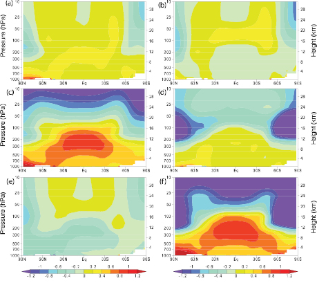
Figure 9.1. Zonal mean atmospheric temperature change from 1890 to 1999 (°C per century) as simulated by the PCM model from (a) solar forcing, (b) volcanoes, (c) well-mixed greenhouse gases, (d) tropospheric and stratospheric ozone changes, (e) direct sulphate aerosol forcing and (f) the sum of all forcings. Plot is from 1,000 hPa to 10 hPa (shown on left scale) and from 0 km to 30 km (shown on right). See Appendix 9.C for additional information. Based on Santer et al. 2003a [PoC, JoC, MoS, SRC] ).
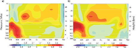
Figure 9.2. The zonal mean equilibrium temperature change (°C) between a present day minus a pre-industrial simulation by the CSIRO atmospheric model coupled to a mixed-layer ocean model from (a) direct forcing from fossil fuel black carbon and organic matter (BC+OM) and (b) the sum of fossil fuel BC+OM and biomass burning. Plot is from 1,000 hPa to 10 hPa (shown on left scale) and from 0 km to 30 km (shown on right). Note the difference in colour scale from Figure 9.1. See Supplementary Material, Appendix 9.C for additional information. Based on Penner et al. 2007 [NPR, SRC, 2007] ).
Greenhouse gas forcing is expected to produce warming in the troposphere, cooling in the stratosphere, and, for transient simulations, somewhat more warming near the surface in the NH due to its larger land fraction, which has a shorter surface response time to the warming than do ocean regions( Figure 9.1 c). The spatial pattern of the transient surface temperature response to greenhouse gas forcing also typically exhibits a land-sea pattern of stronger warming over land, for the same reason (e.g., Cubasch et al., 2001 [NPR, MoS, ARC] ). Sulphate aerosol forcing results in cooling throughout most of the globe, with greater cooling in the NH due to its higher aerosol loading( Figure 9.1 e; see Chapter2 ), thereby partially offsetting the greater NH greenhouse-gas induced warming. The combined effect of tropospheric and stratospheric ozone forcing( Figure 9.1 d) is expected to warm the troposphere, due to increases in tropospheric ozone, and cool the stratosphere, particularly at high latitudes where stratospheric ozone loss has been greatest. Greenhouse gas forcing is also expected to change the hydrological cycle worldwide, leading to disproportionately greater increases in heavy precipitation( Chapter 10 and Section 9.5.4 ), while aerosol forcing can influence rainfall regionally( Section 9.5.4 ).
The simulated responses to natural forcing are distinct from those due to the anthropogenic forcings described above. Solar forcing results in a general warming of the atmosphere( Figure 9.1 a) with a pattern of surface warming that is similar to that expected from greenhouse gas warming, but in contrast to the response to greenhouse warming, the simulated solar-forced warming extends throughout the atmosphere (see, e.g., Cubasch et al., 1997 [JoC, MoS, ARC] ). A number of independent analyses have identified tropospheric changes that appear to be associated with the solar cycle ( van Loon and Shea, 2000 [JoC, ARC] ; Gleisner and Thejll, 2003 [JoC] ; Haigh, 2003 [JoC, ARC] ; White et al., 2003 [JoC, ARC] ; Coughlin and Tung, 2004 [JoC] ;( Labitzke, 2004; ) Crooks and Gray, 2005 [JoC, SRC] ), suggesting an overall warmer and moister troposphere during solar maximum. The peak-to-trough amplitude of the response to the solar cycle globally is estimated to be approximately 0.1°C near the surface. Such variations over the 11-year solar cycle make it is necessary to use several decades of data in detection and attribution studies. The solar cycle also affects atmospheric ozone concentrations with possible impacts on temperatures and winds in the stratosphere, and has been hypothesised to influence clouds through cosmic rays( Section 2.7.1.3 ). Note that there is substantial uncertainty in the identification of climate response to solar cycle variations because the satellite period is short relative to the solar cycle length, and because the response is difficult to separate from internal climate variations and the response to volcanic eruptions ( Gray et al., 2005 [NPR, ARC] ).
Volcanic sulphur dioxide (SO2)emissions ejected into the stratosphere form sulphate aerosols and lead to a forcing that causes a surface and tropospheric cooling and a stratospheric warming that peak several months after a volcanic eruption and last for several years. Volcanic forcing also likely leads to a response in the atmospheric circulation in boreal winter (discussed below) and a reduction in land precipitation ( Robock and Liu, 1994 [JoC, MoS] ; Broccoli et al., 2003 [JoC, MoS, ARC] ; Gillett et al., 2004b [JoC, SRC] ). The response to volcanic forcing causes a net cooling over the 20th century because of variations in the frequency and intensity of volcanic eruptions. This results in stronger volcanic forcing towards the end of the 20th century than early in the 20th century. In the PCM, this increase results in a small warming in the lower stratosphere and near the surface at high latitudes, with cooling elsewhere( Figure 9.1 b).
The net effect of all forcings combined is a pattern of NH temperature change near the surface that is dominated by the positive forcings (primarily greenhouse gases), and cooling in the stratosphere that results predominantly from greenhouse gas and stratospheric ozone forcing( Figure 9.1 f). Results obtained with the CSIRO model( Figure 9.2 )suggest that black carbon, organic matter and biomass aerosols would slightly enhance the NH warming shown in Figure 9.1 f. On the other hand, indirect aerosol forcing from fossil fuel aerosols may be larger than the direct effects that are represented in the CSIRO and PCM models, in which case the NH warming could be somewhat diminished. Also, while land use change may cause substantial forcing regionally and seasonally, its forcing and response are expected to have only a small impact at large spatial scales (Sections 9.3.3.3 and 7.2.2 ;Figures 2.20 and 2.23 ).
The spatial signature of a climate model’s response is seldom very similar to that of the forcing, due in part to the strength of the feedbacks relative to the initial forcing. This comes about because climate system feedbacks vary spatially and because the atmospheric and ocean circulation cause a redistribution of energy over the globe. For example, sea ice albedo feedbacks tend to enhance the high-latitude response of both a positive forcing, such as that of CO2,and a negative forcing such as that of sulphate aerosol (e.g., Mitchell et al., 2001 [NPR] ; Rotstayn and Penner, 2001 [JoC, MoS, SRC] ). Cloud feedbacks can affect both the spatial signature of the response to a given forcing and the sign of the change in temperature relative to the sign of the radiative forcing( Section 8.6 ). Heating by black carbon, for example, can decrease cloudiness ( Ackerman et al., 2000 [JoC] ). If the black carbon is near the surface, it may increase surface temperatures, while at higher altitudes it may reduce surface temperatures ( Hansen et al., 1997 [JoC, MoS, ARC] ; Penner et al., 2003 [JoC, SRC] ). Feedbacks can also lead to differences in the response of different models to a given forcing agent, since the spatial response of a climate model to forcing depends on its representation of these feedbacks and processes. Additional factors that affect the spatial pattern of response include differences in thermal inertia between land and sea areas, and the lifetimes of the various forcing agents. Shorter-lived agents, such as aerosols, tend to have a more distinct spatial pattern of forcing, and can therefore be expected to have some locally distinct response features.
The pattern of response to a radiative forcing can also be altered quite substantially if the atmospheric circulation is affected by the forcing. Modelling studies and data comparisons suggest that volcanic aerosols (e.g., Kirchner et al., 1999 [JoC, MoS] ; Shindell et al., 1999 [PoC, JoC, MoS, ARC] ; Yang and Schlesinger, 2001 [JoC] ; Stenchikov et al., 2006 [JoC, MoS, ARC] ) and greenhouse gas changes (e.g., Fyfe et al., 1999 [JoC, ARC] ; Shindell et al., 1999 [PoC, JoC, MoS, ARC] ; Rauthe et al., 2004 [JoC, MoS] ) can alter the North Atlantic Oscillation (NAO) or the Northern Annular Mode (NAM). For example, volcanic eruptions, with the exception of high-latitude eruptions, are often followed by a positive phase of the NAM or NAO (e.g., Stenchikov et al., 2006 [JoC, MoS, ARC] ) leading to Eurasian winter warming that may reduce the overall cooling effect of volcanic eruptions on annual averages, particularly over Eurasia ( Perlwitz and Graf, 2001 [JoC] ; Stenchikov et al., 2002 [JoC, ARC] ; Shindell et al., 2003 [PoC, JoC, MoS, ARC] ; Stenchikov et al., 2004 [JoC, ARC] ; Oman et al., 2005 [JoC] ; Rind et al., 2005a [JoC, SRC] ; Miller et al., 2006 [PoC, JoC, MoS, ARC] ; Stenchikov et al., 2006 [JoC, MoS, ARC] ). In contrast, NAM or NAO responses to solar forcing vary between studies, some indicating a response, perhaps with dependence of the response on season or other conditions, and some finding no changes ( Shindell et al., 2001a [PoC, JoC, MoS, SRC] ,b; Ruzmaikin and Feynman, 2002 [JoC] ; Tourpali et al., 2003 [JoC, MoS] ; Egorova et al., 2004 [JoC, MoS] ; Palmer et al., 2004 [MoS, SRC] ; Stendel et al., 2006 [JoC, MoS, ARC] ; see also review in Gray et al., 2005 [NPR, ARC] ).
In addition to the spatial pattern, the temporal evolution of the different forcings( Figure 2.23 )generally helps to distinguish between the responses to different forcings. For example, Santer et al. 1996b [PoC, JoC, SRC] ,c) point out that a temporal pattern in the hemispheric temperature contrast would be expected in the second half of the 20th century with the SH warming more than the NH for the first two decades of this period and the NH subsequently warming more than the SH, as a result of changes in the relative strengths of the greenhouse gas and aerosol forcings. However, it should be noted that the integrating effect of the oceans ( Hasselmann, 1976 [JoC, MoS] ) results in climate responses that are more similar in time between different forcings than the forcings are to each other, and that there are substantial uncertainties in the evolution of the hemispheric temperature contrasts associated with sulphate aerosol forcing.
9.2.2.2 Aerosol Scattering and Cloud Feedback in Models and Observations
One line of observational evidence that reflective aerosol forcing has been changing over time comes from satellite observations of changes in top-of-atmosphere outgoing shortwave radiation flux. Increases in the outgoing shortwave radiation flux can be caused by increases in reflecting aerosols, increases in clouds or a change in the vertical distribution of clouds and water vapour, or increases in surface albedo. Increases in aerosols and clouds can cause decreases in surface radiation fluxes and decreases in surface warming. There has been continuing interest in this possibility ( Gilgen et al., 1998 [JoC, MoS, ARC] ;( Stanhill and Cohen, 2001; ) Liepert, 2002 [JoC, ARC] ). Sometimes called ‘global dimming’, this phenomena has reversed since about 1990 ( Pinker et al., 2005 [JoC] ; Wielicki et al., 2005 [JoC, SRC] ; Wild et al., 2005 [JoC, ARC] ; Section 3.4.3 ), but over the entire period from 1984 to 2001, surface solar radiation has increased by about 0.16 Wm–2 yr–1 on average ( Pinker et al., 2005 [JoC] ). Figure 9.3 shows the top-of-atmosphere outgoing shortwave radiation flux anomalies from the MMD at PCMDI, compared to that measured by the Earth Radiation Budget Satellite (ERBS; Wong et al., 2006 [JoC, SRC] ) and inferred from International Satellite Cloud Climatology Project (ISCCP) flux data (FD) ( Zhang et al., 2004 [JoC, MoS] ). The downward trend in outgoing solar radiation is consistent with the long-term upward trend in surface radiation found by Pinker et al. 2005 [JoC] ). The effect of the eruption of Mt. Pinatubo in 1991 results in an increase in the outgoing shortwave radiation flux (and a corresponding dimming at the surface) and its effect has been included in most (but not all) models in the MMD. The ISCCP flux anomaly for the Mt. Pinatubo signal is almost 2 Wm–2 larger than that for ERBS, possibly due to the aliasing of the stratospheric aerosol signal into the ISCCP cloud properties. Overall, the trends from the ISCCP FD (–0.18 with 95% confidence limits of ±0.11 Wm–2 yr–1)and the ERBS data (–0.13 ± 0.08 Wm–2 yr–1)from 1984 to 1999 are not significantly different from each other at the 5% significance level, and are in even better agreement if only tropical latitudes are considered ( Wong et al., 2006 [JoC, SRC] ). These observations suggest an overall decrease in aerosols and/or clouds, while estimates of changes in cloudiness are uncertain (see Section 3.4.3 ). The model-predicted trends are also negative over this time period, but are smaller in most models than in the ERBS observations (which are considered more accurate than the ISCCP FD). Wielicki et al. 2002 [JoC, SRC] ) explain the observed downward trend by decreases in cloudiness, which are not well represented in the models on these decadal time scales ( Chen et al., 2002 [JoC] ; Wielicki et al., 2002 [JoC, SRC] ).
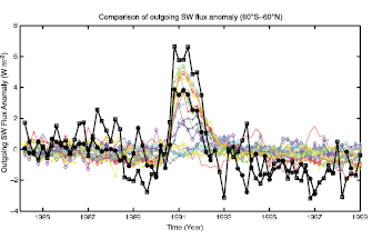
Figure 9.3. Comparison of outgoing shortwave radiation flux anomalies (in Wm–2,calculated relative to the entire time period) from several models in the MMD archive at PCMDI (coloured curves) with ERBS satellite data (black with stars; Wong et al., 2006 [JoC, SRC] ) and with the ISCCP flux data set (black with squares; Zhang et al., 2004 [JoC, MoS] ). Models shown are CCSM3, CGCM3.1(T47), CGCM3.1(T63), CNRM-CM3, CSIRO-MK3.0, FGOALS-g1.0, GFDL-CM2.0, GFDL-CM2.1, GISS-AOM, GISS-EH, GISS-ER, INM-CM3.0, IPSL-CM4, and MRI-CGCM2.3.2 (see Table 8.1 for model details). The comparison is restricted to 60°S to 60°N because the ERBS data are considered more accurate in this region. Note that not all models included the volcanic forcing from Mt. Pinatubo ( 1991 – 1993 ) and so do not predict the observed increase in outgoing solar radiation. See Supplementary Material, Appendix 9.C for additional information.
9.2.2.3 Uncertainty in the Spatial Pattern of Response
Most detection methods identify the magnitude of the space-time patterns of response to forcing (sometimes called ‘fingerprints’) that provide the best fit to the observations. The fingerprints are typically estimated from ensembles of climate model simulations forced with reconstructions of past forcing. Using different forcing reconstructions and climate models in such studies provides some indication of forcing and model uncertainty. However, few studies have examined how uncertainties in the spatial pattern of forcing explicitly contribute to uncertainties in the spatial pattern of the response. For short-lived components, uncertainties in the spatial pattern of forcing are related to uncertainties in emissions patterns, uncertainties in the transport within the climate model or chemical transport model and, especially for aerosols, uncertainties in the representation of relative humidities or clouds. These uncertainties affect the spatial pattern of the forcing. For example, the ratio of the SH to NH indirect aerosol forcing associated with the total aerosol forcing ranges from –0.12 to 0.63 (best guess 0.29) in different studies, and that between ocean and land forcing ranges from 0.03 to 1.85 (see Figure 7.21 ;Rotstayn and Penner, 2001 [JoC, MoS, SRC] ; Chuang et al., 2002 [JoC, MoS] ; Kristjansson, 2002 [NPR, JoC] ; Lohmann and Lesins, 2002 [JoC, ARC] ; Menon et al., 2002a [JoC, MoS, ARC] ; Rotstayn and Liu, 2003 [JoC, SRC] ; Lohmann and Feichter, 2005 [ARC] ).
There are also large uncertainties in the magnitude of low-frequency changes in forcing associated with changes in total solar radiation as well as its spectral variation, particularly on time scales longer than the 11-year cycle. Previous estimates of change in total solar radiation have used sunspot numbers to calculate these slow changes in solar irradiance over the last few centuries, but these earlier estimates are not necessarily supported by current understanding and the estimated magnitude of low-frequency changes has been substantially reduced since the TAR ( Lean et al., 2002 [JoC, MoS, ARC] ; Foukal et al., 2004 [PoC, JoC, ARC] , 2006; Sections 6.6.3.1 and 2.7.1.2 ). In addition, the magnitude of radiative forcing associated with major volcanic eruptions is uncertain and differs between reconstructions ( Sato et al., 1993 [JoC, ARC] ; Andronova et al., 1999 [JoC, MoS, SRC] ; Ammann et al., 2003 [PoC, JoC, MoS, SRC] ), although the timing of the eruptions is well documented.
9.2.2.4 Uncertainty in the Temporal Pattern of Response
Climate model studies have also not systematically explored the effect of uncertainties in the temporal evolution of forcings. These uncertainties depend mainly on the uncertainty in the spatio-temporal expression of emissions, and, for some forcings, fundamental understanding of the possible change over time.
The increasing forcing by greenhouse gases is relatively well known. In addition, the global temporal history of SO2 emissions, which have a larger overall forcing than the other short-lived aerosol components, is quite well constrained. Seven different reconstructions of the temporal history of global anthropogenic sulphur emissions up to 1990 have a relative standard deviation of less than 20% between 1890 and 1990, with better agreement in more recent years. This robust temporal history increases confidence in results from detection and attribution studies that attempt to separate the effects of sulphate aerosol and greenhouse gas forcing( Section 9.4.1 ).
In contrast, there are large uncertainties related to the anthropogenic emissions of other short-lived compounds and their effects on forcing. For example, estimates of historical emissions from fossil fuel combustion do not account for changes in emission factors (the ratio of the emitted gas or aerosol to the fuel burned) of short-lived species associated with concerns over urban air pollution (e.g., van Aardenne et al., 2001 [JoC] ). Changes in these emission factors would have slowed the emissions of nitrogen oxides as well as carbon monoxide after about 1970 and slowed the accompanying increase in tropospheric ozone compared to that represented by a single emission factor for fossil fuel use. In addition, changes in the height of SO2 emissions associated with the implementation of tall stacks would have changed the lifetime of sulphate aerosols and the relationship between emissions and effects. Another example relates to the emissions of black carbon associated with the burning of fossil fuels. The spatial and temporal emissions of black carbon by continent reconstructed by Ito and Penner 2005 [JoC, SRC] ) are significantly different from those reconstructed using the methodology of Novakov et al. 2003 [JoC] ). For example, the emissions in Asia grow significantly faster in the inventory based on Novakov et al. 2003 [JoC] ) compared to those based on Ito and Penner 2005 [JoC, SRC] ). In addition, before 1988 the growth in emissions in Eastern Europe using the Ito and Penner 2005 [JoC, SRC] ) inventory is faster than the growth based on the methodology of Novakov et al. 2003 [JoC] ). Such spatial and temporal uncertainties will contribute to both spatial and temporal uncertainties in the net forcing and to spatial and temporal uncertainties in the distribution of forcing and response.
9.2.3 Implications for Understanding 20th-Century Climate Change
Any assessment of observed climate change that compares simulated and observed responses will be affected by errors and uncertainties in the forcings prescribed in a climate model and its corresponding responses. As noted above, detection studies scale the response patterns to different forcings to obtain the best match to observations. Thus, errors in the magnitude of the forcing or in the magnitude of the model response to a forcing (which is approximately, although not exactly, a function of climate sensitivity), should not affect detection results provided that the large-scale space-time pattern of the response is correct. Attribution studies evaluate the consistency between the model-simulated amplitude of response and that inferred from observations. In the case of uncertain forcings, scaling factors provide information about the strength of the forcing (and response) needed to reproduce the observations, or about the possibility that the simulated pattern or strength of response is incorrect. However, for a model simulation to be considered consistent with the observations given forcing uncertainty, the forcing used in the model should remain consistent with the uncertainty bounds from forward model estimates of forcing.
Detection and attribution approaches that try to distinguish the response to several external forcings simultaneously may be affected by similarities in the pattern of response to different forcings and by uncertainties in forcing and response. Similarities between the responses to different forcings, particularly in the spatial patterns of response, make it more difficult to distinguish between responses to different external forcings, but also imply that the response patterns will be relatively insensitive to modest errors in the magnitude and distribution of the forcing. Differences between the temporal histories of different kinds of forcing (e.g., greenhouse gas versus sulphate aerosol) ameliorate the problem of the similarity between the spatial patterns of response considerably. For example, the spatial response of surface temperature to solar forcing resembles that due to anthropogenic greenhouse gas forcing ( Weatherall and Manabe, 1975 [JoC, MoS] ; Nesme-Ribes et al., 1993 [JoC] ; Cubasch et al., 1997 [JoC, MoS, ARC] ; Rind et al., 2004 [JoC, MoS, SRC] ; Zorita et al., 2005 [JoC, SRC] ). Distinct features of the vertical structure of the responses in the atmosphere to different types of forcing further help to distinguish between the different sources of forcing. Studies that interpret observed climate in subsequent sections use such strategies, and the overall assessment in this chapter uses results from a range of climate variables and observations.
Many detection studies attempt to identify in observations both temporal and spatial aspects of the temperature response to a given set of forcings because the combined space-time responses tend to be more distinct than either the space-only or the time-only patterns of response. Because the emissions and burdens of different forcing agents change with time, the net forcing and its rate of change vary with time. Although explicit accounting for uncertainties in the net forcing is not available (see discussion in Sections 9.2.2.3 and 9.2.2.4 ), models often employ different implementations of external forcing. Detection and attribution studies using such simulations suggest that results are not very sensitive to moderate forcing uncertainties. A further problem arises due to spurious temporal correlations between the responses to different forcings that arise from sampling variability. For example, spurious correlation between the climate responses to solar and volcanic forcing over parts of the 20th century ( North and Stevens, 1998 [JoC] ) can lead to misidentification of one as the other, as in Douglass and Clader 2002 [JoC] ).
The spatial pattern of the temperature response to aerosol forcing is quite distinct from the spatial response pattern to CO2 in some models and diagnostics ( Hegerl et al., 1997 [JoC, SRC] ), but less so in others ( Reader and Boer, 1998 [JoC] ; Tett et al., 1999 [JoC, SRC] ; Hegerl et al., 2000 [JoC, MoS, SRC] ; Harvey, 2004 [JoC] ). If it is not possible to distinguish the spatial pattern of greenhouse warming from that of fossil-fuel related aerosol cooling, the observed warming over the last century could be explained by large greenhouse warming balanced by large aerosol cooling or alternatively by small greenhouse warming with very little or no aerosol cooling. Nevertheless, estimates of the amplitude of the response to greenhouse forcing in the 20th century from detection studies are quite similar, even though the simulated responses to aerosol forcing are model dependent ( Gillett et al., 2002a [JoC, SRC] ; Hegerl and Allen, 2002 [JoC, MoS, SRC] ). Considering three different climate models, Stott et al. 2006c [JoC, MoS, SRC] ) conclude that an important constraint on the possible range of responses to aerosol forcing is the temporal evolution of the global mean and hemispheric temperature contrast as was suggested by Santer et al. 1996a [NPR, PoC, SRC] ; see also Section 9.4.1.5 ).
9.2.4 Summary
The uncertainty in the magnitude and spatial pattern of forcing differs considerably between forcings. For example, well-mixed greenhouse gas forcing is relatively well constrained and spatially homogeneous. In contrast, uncertainties are large for many non-greenhouse gas forcings. Inverse model studies, which use methods closely related to those used in climate change detection research, indicate that the magnitude of the total net aerosol forcing has a likely range of –1.7 to –0.1 Wm–2.As summarised in Chapter2 ,forward calculations of aerosol radiative forcing, which do not depend on knowledge of observed climate change or the ability of climate models to simulate the transient response to forcings, provide results (–2.2 to –0.5 Wm–2;5 to 95%) that are quite consistent with inverse estimates; the uncertainty ranges from inverse and forward calculations are different due to the use of different information. The large uncertainty in total aerosol forcing makes it more difficult to accurately infer the climate sensitivity from observations( Section 9.6 ). It also increases uncertainties in results that attribute cause to observed climate change( Section 9.4.1.4 ), and is in part responsible for differences in probabilistic projections of future climate change( Chapter 10 ). Forcings from black carbon, fossil fuel organic matter and biomass burning aerosols, which have not been considered in most detection studies performed to date, are likely small but with large uncertainties relative to the magnitudes of the forcings.
Uncertainties also differ between natural forcings and sometimes between different time scales for the same forcing. For example, while the 11-year solar forcing cycle is well documented, lower-frequency variations in solar forcing are highly uncertain. Furthermore, the physics of the response to solar forcing and some feedbacks are still poorly understood. In contrast, the timing and duration of forcing due to aerosols ejected into the stratosphere by large volcanic eruptions is well known during the instrumental period, although the magnitude of that forcing is uncertain.
Differences in the temporal evolution and sometimes the spatial pattern of climate response to external forcing make it possible, with limitations, to separate the response to these forcings in observations, such as the responses to greenhouse gas and sulphate aerosol forcing. In contrast, the climate response and temporal evolution of other anthropogenic forcings is more uncertain, making the simulation of the climate response and its detection in observations more difficult. The temporal evolution, and to some extent the spatial and vertical pattern, of the climate response to natural forcings is also quite different from that of anthropogenic forcing. This makes it possible to separate the climate response to solar and volcanic forcing from the response to anthropogenic forcing despite the uncertainty in the history of solar forcing noted above.
9.3 Understanding Pre-Industrial Climate Change
9.3.1 Why Consider Pre-Industrial Climate Change?
The Earth system has experienced large-scale climate changes in the past( Chapter6 )that hold important lessons for the understanding of present and future climate change. These changes resulted from natural external forcings that, in some instances, triggered strong feedbacks as in the case of the LGM (see Chapter6 ). Past periods offer the potential to provide information not available from the instrumental record, which is affected by anthropogenic as well as natural external forcings and is too short to fully understand climate variability and major climate system feedbacks on inter-decadal and longer time scales. Indirect indicators (‘proxy data’ such as tree ring width and density) must be used to infer climate variations( Chapter6 )prior to the instrumental era( Chapter3 ). A complete description of these data and of their uncertainties can be found in Chapter6 .
The discussion here is restricted to several periods in the past for which modelling and observational evidence can be compared to test understanding of the climate response to external forcings. One such period is the last millennium, which places the recent instrumental record in a broader context (e.g., Mitchell et al., 2001 [NPR] ). The analysis of the past 1 kyr focuses mainly on the climate response to natural forcings (changes in solar radiation and volcanism) and on the role of anthropogenic forcing during the most recent part of the record. Two time periods analysed in the Paleoclimate Modelling Intercomparison Project (PMIP, Joussaume and Taylor, 1995 [NPR, ARC] ; PMIP2, Harrison et al., 2002 [JoC, MoS, SRC] ) are also considered, the mid-Holocene (6 ka) and the LGM (21 ka). Both periods had a substantially different climate compared to the present, and there is relatively good information from data synthesis and model simulation experiments ( Braconnot et al., 2004 [NPR, MoS, SRC] ; Cane et al., 2006 [JoC, MoS] ). An increased number of simulations using EMICs or Atmosphere-Ocean General Circulation Models (AOGCMs) that are the same as, or related to, the models used in simulations of the climates of the 20th and 21st centuries are available for these periods.
9.3.2 What Can be Learned from the Last Glacial Maximum and the Mid-Holocene?
Relatively high-quality global terrestrial climate reconstructions exist for the LGM and the mid-Holocene and as part of the Global Palaeovegetation Mapping (BIOME 6000) project ( (Prentice and Webb, 1998; ) ( Prentice and Jolly, 2000 ) ). The Climate: Long-range Investigation, Mapping and Prediction ( CLIMAP, 1981 [NPR] ) reconstruction of LGM sea surface temperatures has also been improved( Chapter6 ). The LGM climate was colder and drier than at present as is indicated by the extensive tundra and steppe vegetation that existed during this period. Most LGM proxy data suggest that the tropical oceans were colder by about 2°C than at present, and that the frontal zones in the SH and NH were shifted equatorward ( Kucera et al., 2005 [JoC] ), even though large differences are found between temperature estimates from the different proxies in the North Atlantic.
Several new AOGCM simulations of the LGM have been produced since the TAR. These simulations show a global cooling of approximately 3.5°C to 5.2°C when LGM greenhouse gas and ice sheet boundary conditions are specified( Chapter6 ), which is within the range (–1.8°C to –6.5°C) of PMIP results from simpler models that were discussed in the TAR ( McAvaney et al., 2001 [NPR, MoS, ARC] ). Only one simulation exhibits a very strong response with a cooling of approximately 10°C ( Kim et al., 2002 [JoC, MoS, ARC] ). All of these simulations exhibit a strongly damped hydrological cycle relative to that of the modern climate, with less evaporation over the oceans and continental-scale drying over land. Changes in greenhouse gas concentrations may account for about half of the simulated tropical cooling ( Shin et al., 2003 [JoC, MoS] ), and for the production of colder and saltier water found at depth in the Southern Ocean ( Liu et al., 2005 [JoC, MoS] ). Most LGM simulations with coupled models shift the deep-water formation in the North Atlantic southward, but large differences exist between models in the intensity of the Atlantic meridional overturning circulation. Including vegetation changes appears to improve the realism of LGM simulations ( Wyputta and McAvaney, 2001 [JoC, MoS, ARC] ). Furthermore, including the physiological effect of the atmospheric CO2 concentration on vegetation has a non-negligible impact ( Levis et al., 1999 [JoC] ) and is necessary to properly represent changes in global forest ( Harrison and Prentice, 2003 [MoS] ) and terrestrial carbon storage (e.g., Kaplan et al., 2002 [JoC, MoS] ; Joos et al., 2004 [PoC, JoC, MoS, SRC] ; see also Chapter6 ). To summarise, despite large uncertainties, LGM simulations capture the broad features found in palaeoclimate data, and better agreement is obtained with new coupled simulations using more recent models and more complete feedbacks from ocean, sea ice and land surface characteristics such as vegetation and soil moisture( Chapter6 ).
Closer to the present, during the mid-Holocene, one of the most noticeable indications of climate change is the northward extension of northern temperate forest ( Bigelow et al., 2003 [JoC] ), which reflects warmer summers than at present. In the tropics the more vegetated conditions inferred from pollen records in the now dry sub-Saharan regions indicate wetter conditions due to enhanced summer monsoons (see Braconnot et al., 2004 [NPR, MoS, SRC] for a review). Simulations of the mid-Holocene with AOGCMs (see Section 9.2.1.3 for forcing) produce an amplification of the mean seasonal cycle of temperature of approximately 0.5°C to 0.7°C. This range is slightly smaller than that obtained using atmosphere-only models in PMIP1 (~0.5°C to ~1.2°C) due to the thermal response of the ocean ( Braconnot et al., 2000 [JoC, SRC] ). Simulated changes in the ocean circulation have strong seasonal features with an amplification of the sea surface temperature (SST) seasonal cycle of 1°C to 2°C in most places within the tropics ( Zhao et al., 2005 [JoC, MoS] ), influencing the Indian and African monsoons. Over West Africa, AOGCM-simulated changes in annual mean precipitation are about 5 to 10% larger than for atmosphere-only simulations, and in better agreement with data reconstructions ( Braconnot et al., 2004 [NPR, MoS, SRC] ). Results for the Indian and Southwest Asian monsoon are less consistent between models.
As noted in the TAR ( McAvaney et al., 2001 [NPR, MoS, ARC] ), vegetation change during the mid-Holocene likely triggered changes in the hydrological cycle, explaining the wet conditions that prevailed in the Sahel region that were further enhanced by ocean feedbacks ( Ganopolski et al., 1998 [JoC, ARC] ; Braconnot et al., 1999 [JoC, SRC] ), although soil moisture may have counteracted some of these feedbacks ( Levis et al., 2004 [JoC, MoS, ARC] Wohlfahrt et al. 2004 [JoC, SRC] ) show that at middle and high latitudes the vegetation and ocean feedbacks enhanced the warming in spring and autumn by about 0.8°C. However, models have a tendency to overestimate the mid-continental drying in Eurasia, which is further amplified when vegetation feedbacks are included ( Wohlfahrt et al., 2004 [JoC, SRC] ).
Awide range of proxies containing information about ENSO variability during the mid-Holocene is now also available( Section 6.5.3 ). These data suggest that ENSO variability was weaker than today prior to approximately 5 kyr before present ( Moy et al., 2002 [JoC] and references therein; Tudhope and Collins, 2003 [JoC, MoS, ARC] ). Several studies have attempted to analyse these changes in interannual variability from model simulations. Even though some results are controversial, a consistent picture has emerged for the mid-Holocene, for which simulations produce reduced variability in precipitation over most ocean regions in the tropics ( Liu et al., 2000 [JoC, MoS] ; Braconnot et al., 2004 [NPR, MoS, SRC] ; Zhao et al., 2005 [JoC, MoS] ). Results obtained with the Cane-Zebiak model suggest that the Bjerknes 1969 [JoC] ) feedback mechanism may be a key element of the ENSO response in that model. The increased mid-Holocene solar heating in boreal summer leads to more warming in the western than in the eastern Pacific, which strengthens the trade winds and inhibits the development of ENSO ( Clement et al., 2000 [JoC, SRC] , 2004 ). Atmosphere-Ocean General Circulation Models also tend to simulate less intense ENSO events, in qualitative agreement with data, although there are large differences in magnitude and proposed mechanisms, and inconsistent responses of the associated teleconnections ( Otto-Bliesner, 1999 [JoC, SRC] ; Liu et al., 2000 [JoC, MoS] ; Kitoh and Murakami, 2002 [JoC, MoS, ARC] ; Otto-Bliesner et al., 2003 [JoC, MoS, SRC] ).
9.3.3 What Can be Learned from the Past 1,000 Years?
External forcing relative to the present is generally small for the last millennium when compared to that for the mid-Holocene and LGM. Nonetheless, there is evidence that climatic responses to forcing, together with natural internal variability of the climate system, produced several well-defined climatic events, such as the cool conditions during the 17th century or relatively warm periods early in the millennium.
9.3.3.1 Evidence of External Influence on the Climate Over the Past 1,000 Years
Asubstantial number of proxy reconstructions of annual or decadal NH mean surface temperature are now available (see Figure 6.11 ,and the reviews by Jones et al., 2001 [PoC, JoC, ARC] and Jones and Mann, 2004 [PoC, JoC, ARC] ). Several new reconstructions have been published, some of which suggest larger variations over the last millennium than assessed in the TAR, but uncertainty remains in the magnitude of inter-decadal to inter-centennial variability. This uncertainty arises because different studies rely on different proxy data or use different reconstruction methods( Section 6.6.1 ). Nonetheless, NH mean temperatures in the second half of the 20th century were likely warmer than in any other 50-year period in the last 1.3 kyr( Chapter6 ), and very likely warmer than any such period in the last 500 years. Temperatures subsequently decreased, and then rose rapidly during the most recent 100 years. This long-term tendency is punctuated by substantial shorter-term variability( Figure 6.10 ). For example, cooler conditions with temperatures 0.5°C to 1°C below the 20th-century mean value are found in the 17th and early 18th centuries.
Anumber of simulations of the last millennium( Figure 6.13 )have been performed using a range of models, including some simulations with AOGCMs (e.g., Crowley, 2000 [PoC, JoC] ; Goosse and Renssen, 2001 [JoC, SRC] ; Bertrand et al., 2002 [JoC, ARC] ; Bauer et al., 2003 [JoC, MoS, ARC] ; Gerber et al., 2003 [JoC, MoS] ; see also Gonzalez-Rouco et al., 2003 [JoC, MoS, SRC] ; Jones and Mann, 2004 [PoC, JoC, ARC] ; Zorita et al., 2004 [MoS, SRC] ; Weber, 2005 [MoS] ; Tett et al., 2007 [JoC, MoS, SRC, 2007] ). These simulations use different reconstructions of external forcing, particularly solar, volcanic and greenhouse gas forcing, and often include land use changes (e.g., Bertrand et al., 2002 [JoC, ARC] ; Stendel et al., 2006 [JoC, MoS, ARC] ; Tett et al., 2007 [JoC, MoS, SRC, 2007] ). While the use of different models and forcing reconstructions leads to differences, the simulated evolution of the NH annual mean surface temperature displays some common characteristics between models that are consistent with the broad features of the data (Figures 6.13 and 9.4 ). For example, all simulations show relatively cold conditions during the period around 1675 to 1715 in response to natural forcing, which is in qualitative agreement with the proxy reconstructions. In all simulations shown in Figure 6.13 ,the late 20th century is warmer than any other multi-decadal period during the last millennium. In addition, there is significant correlation between simulated and reconstructed variability (e.g., Yoshimori et al., 2005 [JoC, MoS, ARC] ). By comparing simulated and observed atmospheric CO2 concentration during the last 1 kyr, Gerber et al. 2003 [JoC, MoS] ) suggest that the amplitude of the temperature evolution simulated by simple climate models and EMICs is consistent with the observed evolution of CO2.Since reconstructions of external forcing are virtually independent from the reconstructions of past temperatures, this broad consistency increases confidence in the broad features of the reconstructions and the understanding of the role of external forcing in recent climate variability. The simulations also show that it is not possible to reproduce the large 20th-century warming without anthropogenic forcing regardless of which solar or volcanic forcing reconstruction is used ( Crowley, 2000 [PoC, JoC] ; Bertrand et al., 2002 [JoC, ARC] ; Bauer et al., 2003 [JoC, MoS, ARC] ; Hegerl et al., 2003 [JoC, SRC] , 2007 ), stressing the impact of human activity on the recent warming.
While there is broad qualitative agreement between simulated and reconstructed temperatures, it is difficult to fully assess model-simulated variability because of uncertainty in the magnitude of historical variations in the reconstructions and differences in the sensitivity to external forcing( Table 8.2 ). The role of internal variability has been found to be smaller than that of the forced variability for hemispheric temperature means at decadal or longer time scales ( Crowley, 2000 [PoC, JoC] ; Hegerl et al., 2003 [JoC, SRC] ; Goosse et al., 2004 [JoC, MoS, SRC] ; Weber et al., 2004 [PoC, JoC, MoS] ; Hegerl et al., 2007 [JoC, SRC, 2007] ; Tett et al., 2007 [JoC, MoS, SRC, 2007] ), and thus internal variability is a relatively small contributor to differences between different simulations of NH mean temperature. Other sources of uncertainty in simulations include model ocean initial conditions, which, for example, explain the warm conditions found in the Zorita et al. 2004 [MoS, SRC] ) simulation during the first part of the millennium ( Goosse et al., 2005 [JoC, MoS, SRC] ; Osborn et al., 2006 [Ambiguous] ).
9.3.3.2 Role of Volcanism and Solar Irradiance
Volcanic eruptions cause rapid decreases in hemispheric and global mean temperatures followed by gradual recovery over several years( Section 9.2.2.1 )in climate simulations driven by volcanic forcing( Figure 6.13 ;Crowley, 2000 [PoC, JoC] ; Bertrand et al., 2002 [JoC, ARC] ; Weber, 2005 [MoS] ; Yoshimori et al., 2005 [JoC, MoS, ARC] ; Tett et al., 2007 [JoC, MoS, SRC, 2007] ). These simulated changes appear to correspond to cool episodes in proxy reconstructions( Figure 6.13 ). This suggestive correspondence has been confirmed in comparisons between composites of temperatures following multiple volcanic eruptions in simulations and reconstructions ( Hegerl et al., 2003 [JoC, SRC] ; Weber, 2005 [MoS] ). In addition, changes in the frequency of large eruptions result in climate variability on decadal and possibly longer time scales ( Crowley, 2000 [PoC, JoC] ; Briffa et al., 2001 [PoC, JoC, ARC] ; Bertrand et al., 2002 [JoC, ARC] ; Bauer et al., 2003 [JoC, MoS, ARC] ; Weber, 2005 [MoS] Hegerl et al. 2003 [JoC, SRC] ; 2007 ), using a multi-regression approach based on Energy Balance Model (EBM) simulated fingerprints of solar, volcanic and greenhouse gas forcing (Appendix 9.A.1; see also Section 9.4.1.4 for the 20th century), simultaneously detect the responses to volcanic and greenhouse gas forcing in a number of proxy reconstructions of average NH mean annual and growing season temperatures( Figure 9.4 )with high significance. They find that a high percentage of decadal variance in the reconstructions used can be explained by external forcing (between 49 and 70% of decadal variance depending upon the reconstruction).
Figure 9.4. Contribution of external forcing to several high-variance reconstructions of NH temperature anomalies, ( Esper et al., 2002 [PoC, JoC, ARC] ; Briffa et al., 2001 [PoC, JoC, ARC] ; Hegerl et al., 2007 [JoC, SRC, 2007] , termed CH-blend and CH-blend long; and Moberg et al., 2005 [JoC] ). The top panel compares reconstructions to an EBM simulation (equilibrium climate sensitivity of 2.5°C) of NH 30°N to 90°N average temperature, forced with volcanic, solar and anthropogenic forcing. All timeseries are centered on the 1500 - 1925 average. Instrumental temperature data are shown by a green line (centered to agree with CH-blend average over the period 1880 - 1960 ). The displayed data are low-pass filtered (20-year cutoff) for clarity. The bottom panel shows the estimated contribution of the response to volcanic (blue lines with blue uncertainty shade), solar (green) and greenhouse gas (GHG) and aerosol forcing (red line with yellow shades, aerosol only in 20th century) to each reconstruction (all timeseries are centered over the analysis period). The estimates are based on multiple regression of the reconstructions on fingerprints for individual forcings. The contributions to different reconstructions are indicated by different line styles (Briffa et al.: solid, fat; Esper et al.: dotted; Moberg: dashed; CH-blend: solid, thin; with shaded 90% confidence limits around best estimates for each detectable signal). All reconstructions show a highly significant volcanic signal, and all but Moberg et al. (which ends in 1925 ) show a detectable greenhouse gas signal at the 5% significance level. The latter shows a detectable greenhouse gas signal with less significance. Only Moberg et al. contains a detectable solar signal (only shown for these data and CH-blend, where it is not detectable). All data are decadally averaged. The reconstructions represent slightly different regions and seasons: Esper et al. 2002 [PoC, JoC, ARC] ) is calibrated to 30°N to 90°N land temperature, CH-blend and CH-blend long ( Hegerl et al., 2007 [JoC, SRC, 2007] ) to 30°N to 90°N mean temperature and Moberg et al. 2005 [JoC] ) to 0° to 90°N temperature. From Hegerl et al. 2007 [JoC, SRC, 2007] ).
There is more uncertainty regarding the influence of solar forcing. In addition to substantial uncertainty in the timing and amplitude of solar variations on time scales of several decades to centuries, which has increased since the TAR although the estimate of solar forcing has been revised downwards (Sections 9.2.1.3 and 2.7.1 ), uncertainty also arises because the spatial response of surface temperature to solar forcing resembles that due to greenhouse gas forcing( Section 9.2.3 ). Analyses that make use of differences in the temporal evolution of solar and volcanic forcings are better able to distinguish between the two( Section 9.2.3 ;see also Section 9.4.1.5 for the 20th century). In such an analysis, solar forcing can only be detected and distinguished from the effect of volcanic and greenhouse gas forcing over some periods in some reconstructions ( Hegerl et al., 2003 [JoC, SRC] , 2007 ), although the effect of solar forcing has been detected over parts of the 20th century in some time-space analyses( Section 9.4.1.5 )and there are similarities between regressions of solar forcing on model simulations and several proxy reconstructions ( Weber, 2005 [MoS] ; see also Waple, 2002 [PoC, JoC, MoS] ). A model simulation ( Shindell et al., 2003 [PoC, JoC, MoS, ARC] ) suggests that solar forcing may play a substantial role in regional anomalies due to dynamical feedbacks. These uncertainties in the contribution of different forcings to climatic events during the last millennium reflect substantial uncertainty in knowledge about past solar and volcanic forcing, as well as differences in the way these effects are taken into account in model simulations.
Overall, modelling and detection and attribution studies confirm a role of volcanic, greenhouse gas and probably solar forcing in explaining the broad temperature evolution of the last millennium, although the role of solar forcing has recently been questioned ( Foukal et al., 2006 [PoC, JoC, ARC] ). The variability that remains in proxy reconstructions after estimates of the responses to external forcing have been removed is broadly consistent with AOGCM-simulated internal variability (e.g., Hegerl et al., 2003 [JoC, SRC] , 2007 ), providing a useful check on AOGCMs even though uncertainties are large. Such studies also help to explain episodes during the climate of the last millennium. For example, several modelling studies suggest that volcanic activity has a dominant role in explaining the cold conditions that prevailed from 1675 to 1715 ( Andronova et al., 2007 [NPR, SRC, 2007] ; Yoshimori et al., 2005 [JoC, MoS, ARC] ). In contrast, Rind et al. 2004 [JoC, MoS, SRC] ) estimate from model simulations that the cooling relative to today was primarily associated with reduced greenhouse gas forcing, with a substantial contribution from solar forcing.
There is also some evidence from proxy data that the response to external forcing may influence modes of climate variability. For example, Cobb et al. 2003 [JoC] ), using fossil corals, attempt to extend the ENSO record back through the last millennium. They find that ENSO events may have been as frequent and intense during the mid-17th century as during the instrumental period, with events possibly rivalling the strong 1997 – 1998 event. On the other hand, there are periods during the 12th and 14th centuries when there may have been significantly less ENSO variability, a period during which there were also cooler conditions in the northeast Pacific ( MacDonald and Case, 2005 [JoC] ) and evidence of droughts in central North America ( Cook et al., 2004 [PoC, JoC, ARC] Cobb et al. 2003 [JoC] ) find that fluctuations in reconstructed ENSO variability do not appear to be correlated in an obvious way with mean state changes in the tropical Pacific or global mean climate, while Adams et al. 2003 [PoC, JoC, MoS, SRC] ) find statistical evidence for an El Niño-like anomaly during the first few years following explosive tropical volcanic eruptions. The Cane-Zebiak model simulates changes similar to those in the Cobb et al. 2003 [JoC] ) data when volcanism and solar forcing are accounted for, supporting the link with volcanic forcing over the past millennium ( Mann et al., 2005 [PoC, JoC, MoS, SRC] ). However, additional studies with different models are needed to fully assess this relationship, since previous work was less conclusive ( Robock, 2000 [JoC] ).
Extratropical variability also appears to respond to volcanic forcing. During the winter following a large volcanic eruption, the zonal circulation may be more intense, causing a relative warming over the continents during the cold season that could partly offset the direct cooling due to the volcanic aerosols (Sections 9.2.2.1 and 8.4.1 ;Robock, 2000 [JoC] ; Shindell et al., 2003 [PoC, JoC, MoS, ARC] ). A tendency towards the negative NAO state during periods of reduced solar input is found in some reconstructions of this pattern for the NH ( Shindell et al., 2001b [JoC, MoS] ; Luterbacher et al., 2002 [ARC] , 2004; Stendel et al., 2006 [JoC, MoS, ARC] ), possibly implying a solar forcing role in some long-term regional changes, such as the cooling over the NH continents around 1700 ( Shindell et al., 2001b [JoC, MoS] ; Section 9.2.2 ). Indications of changes in ENSO variability during the low solar irradiance period of the 17th to early 18th centuries are controversial (e.g., D’Arrigo et al., 2005 [JoC] ).
9.3.3.3 Other Forcings and Sources of Uncertainties
In addition to forcing uncertainties discussed above, a number of other uncertainties affect the understanding of pre-industrial climate change. For example, land cover change may have influenced the pre-industrial climate ( Bertrand et al., 2002 [JoC, ARC] ; Bauer et al., 2003 [JoC, MoS, ARC] ), leading to a regional cooling of 1°C to 2°C in winter and spring over the major agricultural regions of North America and Eurasia in some model simulations, when pre-agriculture vegetation was replaced by present-day vegetation ( Betts, 2001 [MoS, SRC] ). The largest anthropogenic land cover changes involve deforestation( Chapter2 ). The greatest proportion of deforestation has occurred in the temperate regions of the NH ( Ramankutty and Foley, 1999 [JoC, MoS, ARC] ; Goldewijk, 2001 [JoC, MoS] ). Europe had cleared about 80% of its agricultural area by 1860, but over half of the forest removal in North America took place after 1860 ( Betts, 2001 [MoS, SRC] ), mainly in the late 19th century ( Stendel et al., 2006 [JoC, MoS, ARC] ). During the past two decades, the CO2 flux caused by land use changes has been dominated by tropical deforestation( Section 7.3.2.1.2 ). Climate model simulations suggest that the effect of land use change was likely small at hemispheric and global scales, estimated variously as –0.02°C relative to natural pre-agricultural vegetation ( Betts, 2001 [MoS, SRC] ), less than –0.1°C since 1700 ( Stendel et al., 2006 [JoC, MoS, ARC] ) and about –0.05°C over the 20th century and too small to be detected statistically in observed trends ( Matthews et al., 2004 [JoC, ARC] ). However, the latter authors did find a larger cooling effect since 1700 of between –0.06°C and –0.22°C when they explored the sensitivity to different representations of land cover change.
Oceanic processes and ocean-atmosphere interaction may also have played a role in the climate evolution during the last millennium ( Delworth and Knutson, 2000 [JoC, MoS, SRC] ; Weber et al., 2004 [PoC, JoC, MoS] ; van der Schrier and Barkmeijer, 2005 [JoC] ). Climate models generally simulate a weak to moderate increase in the intensity of the oceanic meridional overturning circulation in response to a decrease in solar irradiance ( Cubasch et al., 1997 [JoC, MoS, ARC] ; Goosse and Renssen, 2004 [JoC, MoS, SRC] ; Weber et al., 2004 [PoC, JoC, MoS] ). A delayed response to natural forcing due to the storage and transport of heat anomalies by the deep ocean has been proposed to explain the warm Southern Ocean around the 14th to 15th centuries ( Goosse et al., 2004 [JoC, MoS, SRC] ).
9.3.4 Summary
Considerable progress has been made since the TAR in understanding the response of the climate system to external forcings. Periods like the mid-Holocene and the LGM are now used as benchmarks for climate models that are used to simulate future climate( Chapter6 ). While considerable uncertainties remain in the climate reconstructions for these periods, and in the boundary conditions used to force climate models, comparisons between simulated and reconstructed conditions in the LGM and mid-Holocene demonstrate that models capture the broad features of changes in the temperature and precipitation patterns. These studies have also increased understanding of the roles of ocean and vegetation feedbacks in determining the response to solar and greenhouse gas forcing. Moreover, although proxy data on palaeoclimatic interannual to multi-decadal variability during these periods remain very uncertain, there is an increased appreciation that external forcing may, in the past, have affected climatic variability such as that associated with ENSO.
The understanding of climate variability and change, and its causes during the past 1 kyr, has also improved since the TAR ( IPCC, 2001 [NPR] ). There is consensus across all millennial reconstructions on the timing of major climatic events, although their magnitude remains somewhat uncertain. Nonetheless, the collection of reconstructions from palaeodata, which is larger and more closely scrutinised than that available for the TAR, indicates that it is likely that NH average temperatures during the second half of the 20th century were warmer than any other 50-year period during the past 1.3 kyr( Chapter6 ). While uncertainties remain in temperature and forcing reconstructions, and in the models used to estimate the responses to external forcings, the available detection studies, modelling and other evidence support the conclusion that volcanic and possibly solar forcings have very likely affected NH mean temperature over the past millennium and that external influences explain a substantial fraction of inter-decadal temperature variability in the past. The available evidence also indicates that natural forcing may have influenced the climatic conditions of individual periods, such as the cooler conditions around 1700 . The climate response to greenhouse gas increases can be detected in a range of proxy reconstructions by the end of the records.
When driven with estimates of external forcing for the last millennium, AOGCMs simulate changes in hemispheric mean temperature that are in broad agreement with proxy reconstructions (given their uncertainties), increasing confidence in the forcing reconstructions, proxy climate reconstructions and models. In addition, the residual variability in the proxy climate reconstructions that is not explained by forcing is broadly consistent with AOGCM-simulated internal variability. Overall, the information on temperature change over the last millennium is broadly consistent with the understanding of climate change in the instrumental era.
9.4 Understanding of Air Temperature Change During the Industrial Era
9.4.1 Global-Scale Surface Temperature Change
9.4.1.1 Observed Changes
Six additional years of observations since the TAR( Chapter3 )show that temperatures are continuing to warm near the surface of the planet. The annual global mean temperature for every year since the TAR has been among the 10 warmest years since the beginning of the instrumental record. The global mean temperature averaged over land and ocean surfaces warmed by 0.76°C ± 0.19°C between the first 50 years of the instrumental record ( 1850 – 1899 ) and the last 5 years ( 2001 – 2005 )( Chapter3 ;with a linear warming trend of 0.74°C ± 0.18°C over the last 100 years ( 1906 – 2005 )). The rate of warming over the last 50 years is almost double that over the last 100 years (0.13°C ± 0.03°C vs 0.07°C ± 0.02°C per decade; Chapter3 ). The larger number of proxy reconstructions from palaeodata than were available for the TAR indicate that it is very likely that average NH temperatures during the second half of the 20th century were warmer than any other 50-year period in the last 500 years and it is likely that this was the warmest period in the past 1.3 kyr( Chapter6 ). Global mean temperature has not increased smoothly since 1900 as would be expected if it were influenced only by forcing from increasing greenhouse gas concentrations (i.e., if natural variability and other forcings did not have a role; see Section 9.2.1 ; Chapter2 ). A rise in near-surface temperatures also occurred over several decades during the first half of the 20th century, followed by a period of more than three decades when temperatures showed no pronounced trend( Figure 3.6 ). Since the mid- 1970 s, land regions have warmed at a faster rate than oceans in both hemispheres( Figure 3.8 )and warming over the SH was smaller than that over the NH during this period( Figure 3.6 ), while warming rates during the early 20th century were similar over land and ocean.
9.4.1.2 Simulations of the 20th Century
There are now a greater number of climate simulations from AOGCMs for the period of the global surface instrumental record than were available for the TAR, including a greater variety of forcings in a greater variety of combinations. These simulations used models with different climate sensitivities, rates of ocean heat uptake and magnitudes and types of forcings (Supplementary Material, Table S9.1). Figure 9.5 shows that simulations that incorporate anthropogenic forcings, including increasing greenhouse gas concentrations and the effects of aerosols, and that also incorporate natural external forcings provide a consistent explanation of the observed temperature record, whereas simulations that include only natural forcings do not simulate the warming observed over the last three decades. A variety of different forcings is used in these simulations. For example, some anthropogenically forced simulations include both the direct and indirect effects of sulphate aerosols whereas others include just the direct effect, and the aerosol forcing that is calculated within models differs due to differences in the representation of physics. Similarly, the effects of tropospheric and stratospheric ozone changes are included in some simulations but not others, and a few simulations include the effects of carbonaceous aerosols and land use changes, while the naturally forced simulations include different representations of changing solar and volcanic forcing. Despite this additional uncertainty, there is a clear separation in Figure 9.5 between the simulations with anthropogenic forcings and those without.
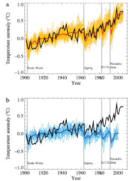
Figure 9.5. Comparison between global mean surface temperature anomalies (°C) from observations (black) and AOGCM simulations forced with (a) both anthropogenic and natural forcings and (b) natural forcings only. All data are shown as global mean temperature anomalies relative to the period 1901 to 1950, as observed (black, Hadley Centre/Climatic Research Unit gridded surface temperature data set (HadCRUT3); Brohan et al., 2006 [JoC, MoS] ) and, in (a) as obtained from 58 simulations produced by 14 models with both anthropogenic and natural forcings. The multi-model ensemble mean is shown as a thick red curve and individual simulations are shown as thin yellow curves. Vertical grey lines indicate the timing of major volcanic events. Those simulations that ended before 2005 were extended to 2005 by using the first few years of the IPCC Special Report on Emission Scenarios (SRES) A1B scenario simulations that continued from the respective 20th-century simulations, where available. The simulated global mean temperature anomalies in (b) are from 19 simulations produced by five models with natural forcings only. The multi-model ensemble mean is shown as a thick blue curve and individual simulations are shown as thin blue curves. Simulations are selected that do not exhibit excessive drift in their control simulations (no more than 0.2°C per century). Each simulation was sampled so that coverage corresponds to that of the observations. Further details of the models included and the methodology for producing this figure are given in the Supplementary Material, Appendix 9.C .After Stott et al. 2006b [JoC, MoS, SRC] ).
Global mean and hemispheric-scale temperatures on multi-decadal time scales are largely controlled by external forcings ( Stott et al., 2000 [JoC, MoS, SRC] ). This external control is demonstrated by ensembles of model simulations with identical forcings (whether anthropogenic or natural) whose members exhibit very similar simulations of global mean temperature on multi-decadal time scales (e.g., Stott et al., 2000 [JoC, MoS, SRC] ; Broccoli et al., 2003 [JoC, MoS, ARC] ; Meehl et al., 2004 [JoC, MoS, ARC] ). Larger interannual variations are seen in the observations than in the ensemble mean model simulation of the 20th century because the ensemble averaging process filters out much of the natural internal interannual variability that is simulated by the models. The interannual variability in the individual simulations that is evident in Figure 9.5 suggests that current models generally simulate large-scale natural internal variability quite well, and also capture the cooling associated with volcanic eruptions on shorter time scales. Section 9.4.1.3 assesses the variability of near surface temperature observations and simulations.
The fact that climate models are only able to reproduce observed global mean temperature changes over the 20th century when they include anthropogenic forcings, and that they fail to do so when they exclude anthropogenic forcings, is evidence for the influence of humans on global climate. Further evidence is provided by spatial patterns of temperature change. Figure 9.6 compares observed near-surface temperature trends over the globe (top row) with those simulated by climate models when they include anthropogenic and natural forcing (second row) and the same trends simulated by climate models when only natural forcings are included (third row). The observed trend over the entire 20th century( Figure 9.6 ,top left panel) shows warming almost everywhere with the exception of the southeastern USA, northern North Atlantic, and isolated grid boxes in Africa and South America (see also Figure 3.9 ). Such a pattern of warming is not associated with known modes of internal climate variability. For example, while El Niño or El Niño-like decadal variability results in unusually warm annual temperatures, the spatial pattern associated with such a warming is more structured, with cooling in the North Pacific and South Pacific (see, e.g., Zhang et al., 1997 [JoC] ). In contrast, the trends in climate model simulations that include anthropogenic and natural forcing( Figure 9.6 ,second row) show a pattern of spatially near-uniform warming similar to that observed. There is much greater similarity between the general evolution of the warming in observations and that simulated by models when anthropogenic and natural forcings are included than when only natural forcing is included( Figure 9.6 ,third row). Figure 9.6 (fourth row) shows that climate models are only able to reproduce the observed patterns of zonal mean near-surface temperature trends over the 1901 to 2005 and 1979 to 2005 periods when they include anthropogenic forcings and fail to do so when they exclude anthropogenic forcings. Although there is less warming at low latitudes than at high northern latitudes, there is also less internal variability at low latitudes, which results in a greater separation of the climate simulations with and without anthropogenic forcings.
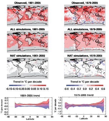
Figure 9.6. Trends in observed and simulated temperature changes (°C) over the 1901 to 2005 (left column) and 1979 to 2005 (right column) periods. First row: trends in observed temperature changes (Hadley Centre/Climatic Research Unit gridded surface temperature data set (HadCRUT3), Brohan et al., 2006 [JoC, MoS] ). Second row: average trends in 58 historical simulations from 14 climate models including both anthropogenic and natural forcings. Third row: average trends in 19 historical simulations from five climate models including natural forcings only. Grey shading in top three rows indicates regions where there are insufficient observed data to calculate a trend for that grid box (see Supplementary Material, Appendix 9.C for further details of data exclusion criteria). Fourth row: average trends for each latitude; observed trends are indicated by solid black curves. Red shading indicates the middle 90% range of trend estimates from the 58 simulations including both anthropogenic and natural forcings (estimated as the range between 4th and 55th of the 58 ranked simulations); blue shading indicates the middle 90% range of trend estimates from the 19 simulations with natural forcings only (estimated as the range between 2nd and 18th of the 19 ranked simulations); for comparison, the dotted black curve in the right-hand plot shows the observed 1901 to 2005 trend. Note that scales are different between columns. The ‘ALL’ simulations were extended to 2005 by adding their IPCC Special Report on Emission Scenarios (SRES) A1B continuation runs where available. Where not available, and in the case of the ‘NAT’ simulations, the mean for the 1996 to 2005 decade was estimated using model output from 1996 to the end of the available runs. In all plots, each climate simulation was sampled so that coverage corresponds to that of the observations. Further details of the models included and the methodology for producing this figure are given in the Supplementary Material, Appendix 9.C .
Climate simulations are consistent in showing that the global mean warming observed since 1970 can only be reproduced when models are forced with combinations of external forcings that include anthropogenic forcings( Figure 9.5 ). This conclusion holds despite a variety of different anthropogenic forcings and processes being included in these models (e.g., Tett et al., 2002 [JoC, MoS, SRC] ; Broccoli et al., 2003 [JoC, MoS, ARC] ; Meehl et al., 2004 [JoC, MoS, ARC] ; Knutson et al., 2006 [JoC, MoS, ARC] ). In all cases, the response to forcing from well-mixed greenhouse gases dominates the anthropogenic warming in the model. No climate model using natural forcings alone has reproduced the observed global warming trend in the second half of the 20th century. Therefore, modelling studies suggest that late 20th-century warming is much more likely to be anthropogenic than natural in origin, a finding which is confirmed by studies relying on formal detection and attribution methods( Section 9.4.1.4 ).
Modelling studies are also in moderately good agreement with observations during the first half of the 20th century when both anthropogenic and natural forcings are considered, although assessments of which forcings are important differ, with some studies finding that solar forcing is more important ( Meehl et al., 2004 [JoC, MoS, ARC] ) while other studies find that volcanic forcing ( Broccoli et al., 2003 [JoC, MoS, ARC] ) or internal variability ( Delworth and Knutson, 2000 [JoC, MoS, SRC] ) could be more important. Differences between simulations including greenhouse gas forcing only and those that also include the cooling effects of sulphate aerosols (e.g., Tett et al., 2002 [JoC, MoS, SRC] ) indicate that the cooling effects of sulphate aerosols may account for some of the lack of observational warming between 1950 and 1970, despite increasing greenhouse gas concentrations, as was proposed by Schwartz 1993 [ARC] ). In contrast, Nagashima et al. 2006 [JoC] ) find that carbonaceous aerosols are required for the MIROC model (see Table 8.1 for a description) to provide a statistically consistent representation of observed changes in near-surface temperature in the middle part of the 20th century. The mid-century cooling that the model simulates in some regions is also observed, and is caused in the model by regional negative surface forcing from organic and black carbon associated with biomass burning. Variations in the Atlantic Multi-decadal Oscillation (see Section 3.6.6 for a more detailed discussion) could account for some of the evolution of global and hemispheric mean temperatures during the instrumental period ( Schlesinger and Ramankutty, 1994 [JoC, ARC] ; Andronova and Schlesinger, 2000 [JoC, SRC] ; Delworth and Mann, 2000 [PoC, JoC, MoS, SRC] Knight et al. 2005 [JoC] ) estimate that variations in the Atlantic Multi-decadal Oscillation could account for up to 0.2°C peak-to-trough variability in NH mean decadal temperatures.
9.4.1.3 Variability of Temperature from Observations and Models
Year-to-year variability of global mean temperatures simulated by the most recent models compares reasonably well with that of observations, as can be seen by comparing observed and modelled variations in Figure 9.5 a. A more quantitative evaluation of modelled variability can be carried out by comparing the power spectra of observed and modelled global mean temperatures. Figure 9.7 compares the power spectrum of observations with the power spectra of transient simulations of the instrumental period. This avoids the need to compare variability estimated from long control runs of models with observed variability, which is difficult because observations are likely to contain a response to external forcings that cannot be reliably removed by subtracting a simple linear trend. The simulations considered contain both anthropogenic and natural forcings, and include most 20th Century Climate in Coupled Models (20C3M) simulations in the MMD at PCMDI. Figure 9.7 shows that the models have variance at global scales that is consistent with the observed variance at the 5% significance level on the decadal to inter-decadal time scales important for detection and attribution. Figure 9.8 shows that this is also generally the case at continental scales, although model uncertainty is larger at smaller scales( Section 9.4.2.2 ).
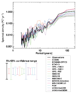
Figure 9.7. Comparison of variability as a function of time scale of annual global mean temperatures (°C2 yr–1)from the observed record (Hadley Centre/Climatic Research Unit gridded surface temperature data set (HadCRUT3), Brohan et al., 2006 [JoC, MoS] ) and from AOGCM simulations including both anthropogenic and natural forcings. All power spectra are estimated using a Tukey-Hanning filter of width 97 years. The model spectra displayed are the averages of the individual spectra estimated from individual ensemble members. The same 58 simulations and 14 models are used as in Figure 9.5a. All models simulate variability on decadal time scales and longer that is consistent with observations at the 10% significance level. Further details of the method of calculating the spectra are given in the Supplementary Material, Appendix 9.C .
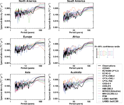
Figure 9.8. As Figure 9.7, except for continental mean temperature. Spectra are calculated in the same manner as Figure 9.7. See the Supplementary Material, Appendix 9.C for a description of the regions and for details of the method used. Models simulate variability on decadal time scales and longer that is consistent with observations in all cases except two models over South America, five models over Asia and two models over Australia (at the 10% significance level).
Detection and attribution studies routinely assess if the residual variability unexplained by forcing is consistent with the estimate of internal variability (e.g., Allen and Tett, 1999 [JoC, MoS, SRC] ; Tett et al., 1999 [JoC, SRC] ; Stott et al., 2001 [JoC, SRC] ; Zwiers and Zhang, 2003 [JoC, SRC] ). Furthermore, there is no evidence that the variability in palaeoclimatic reconstructions that is not explained by forcing is stronger than that in models, and simulations of the last 1 kyr show similar variability to reconstructions( Section 9.3.3.2 ). Chapter8 discusses the simulation of major modes of variability and the extent to which they are simulated by models (including on decadal to inter-decadal time scales).
9.4.1.4 The Influence of Greenhouse Gas and Total Anthropogenic Forcing on Global Surface Temperature
Since the TAR, a large number of studies based on the longer observational record, improved models and stronger signal-to-noise ratio have increased confidence in the detection of an anthropogenic signal in the instrumental record (see, e.g., the recent review by IDAG, 2005 [JoC] ). Many more detection and attribution studies are now available than were available for the TAR, and these have used more recent climate data than previous studies and a much greater variety of climate simulations with more sophisticated treatments of a greater number of both anthropogenic and natural forcings.
Fingerprint studies that use climate change signals estimated from an array of climate models indicate that detection of an anthropogenic contribution to the observed warming is a result that is robust to a wide range of model uncertainty, forcing uncertainties and analysis techniques ( Hegerl et al., 2001 [JoC, SRC] ; Gillett et al., 2002c [NPR, JoC, MoS, SRC] ; Tett et al., 2002 [JoC, MoS, SRC] ; Zwiers and Zhang, 2003 [JoC, SRC] ; IDAG, 2005 [JoC] ; Stone and Allen, 2005b [JoC, MoS, SRC] ; Stone et al., 2007a [JoC, MoS, SRC, 2007] ,b; Stott et al., 2006b [JoC, MoS, SRC] ,c; Zhang et al., 2006 [JoC, MoS, SRC] ). These studies account for the possibility that the agreement between simulated and observed global mean temperature changes could be fortuitous as a result of, for example, balancing too great (or too small) a model sensitivity with a too large (or too small) negative aerosol forcing ( Schwartz, 2004 [MoS, ARC] ; Hansen et al., 2005 [JoC, ARC] ) or a too small (or too large) warming due to solar changes. Multi-signal detection and attribution analyses do not rely on such agreement because they seek to explain the observed temperature changes in terms of the responses to individual forcings, using model-derived patterns of response and a noise-reducing metric (Appendix 9.A) but determining their amplitudes from observations. As discussed in Section 9.2.2.1 ,these approaches make use of differences in the temporal and spatial responses to forcings to separate their effect in observations.
Since the TAR, there has also been an increased emphasis on quantifying the greenhouse gas contribution to observed warming, and distinguishing this contribution from other factors, both anthropogenic, such as the cooling effects of aerosols, and natural, such as from volcanic eruptions and changes in solar radiation.
Acomparison of results using four different models( Figure 9.9 )shows that there is a robust identification of a significant greenhouse warming contribution to observed warming that is likely greater than the observed warming over the last 50 years with a significant net cooling from other anthropogenic forcings over that period, dominated by aerosols. Stott et al. 2006c [JoC, MoS, SRC] ) compare results over the 20th century obtained using the UKMO-HadCM3, PCM (see Table 8.1 for model descriptions) and Geophysical Fluid Dynamics Laboratory (GFDL) R30 models. They find consistent estimates for the greenhouse gas attributable warming over the century, expressed as the difference between temperatures in the last and first decades of the century, of 0.6°C to 1.3°C (5 to 95%) offset by cooling from other anthropogenic factors associated mainly with cooling from aerosols of 0.1°C to 0.7°C and a small net contribution from natural factors over the century of –0.1°C to 0.1°C( Figure 9.9 b). Scaling factors for the model response to three forcings are shown in Figure 9.9 a. A similar analysis for the MIROC3.2 model (see Table 8.1 for a description) finds a somewhat larger warming contribution from greenhouse gases of 1.2°C to 1.5°C offset by a cooling of 0.6°C to 0.8°C from other anthropogenic factors and a very small net natural contribution( Figure 9.9 b). In all cases, the fifth percentile of the warming attributable to greenhouse gases is greater than the observed warming over the last 50 years of the 20th century( Figure 9.9 c).
The detection and estimation of a greenhouse gas signal is also robust to accounting more fully for model uncertainty. An analysis that combines results from three climate models and thereby incorporates uncertainty in the response of these three models (by including an estimate of the inter-model covariance structure in the regression method; Huntingford et al., 2006 [JoC, MoS, SRC] ), supports the results from each of the models individually that it is likely that greenhouse gases would have caused more warming than was observed over the 1950 to 1999 period( Figure 9.9 ,results labelled ‘EIV’). These results are consistent with the results of an earlier analysis, which calculated the mean response patterns from five models and included a simpler estimate of model uncertainty (obtained by a simple rescaling of the variability estimated from a long control run, thereby assuming that inter-model uncertainty has the same covariance structure as internal variability; Gillett et al., 2002c [NPR, JoC, MoS, SRC] ). Both the results of Gillett et al. 2002c [NPR, JoC, MoS, SRC] and Huntingford et al. 2006 [JoC, MoS, SRC] ) indicate that inter-model differences do not greatly increase detection and attribution uncertainties and that averaging fingerprints improves detection results.
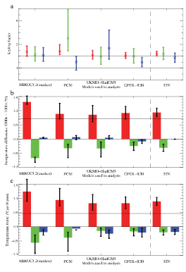
Figure 9.9. Estimated contribution from greenhouse gas (red), other anthropogenic (green) and natural (blue) components to observed global mean surface temperature changes, based on ‘optimal’ detection analyses (Appendix 9.A). (a) 5 to 95% uncertainty limits on scaling factors (dimensionless) based on an analysis over the 20th century, (b) the estimated contribution of forced changes to temperature changes over the 20th century, expressed as the difference between 1990 to 1999 mean temperature and 1900 to 1909 mean temperature (°C) and (c) estimated contribution to temperature trends over 1950 to 1999 (°C per 50 years). The horizontal black lines in (b) and (c) show the observed temperature changes from the Hadley Centre/Climatic Research Unit gridded surface temperature data set (HadCRUT2v; Parker et al., 2004 [ARC] ). The results of full space-time optimal detection analyses ( Nozawa et al., 2005 [JoC, SRC] ; Stott et al., 2006c [JoC, MoS, SRC] ) using a total least squares algorithm ( Allen and Stott, 2003 [JoC, MoS, SRC] ) from ensembles of simulations containing each set of forcings separately are shown for four models, MIROC3.2(medres), PCM, UKMO-HadCM3 and GFDL-R30. Also shown, labelled ‘EIV’, is an optimal detection analysis using the combined spatio-temporal patterns of response from three models (PCM, UKMO-HadCM3 and GFDL-R30) for each of the three forcings separately, thus incorporating inter-model uncertainty ( Huntingford et al., 2006 [JoC, MoS, SRC] ).
Arobust anthropogenic signal is also found in a wide range of climate models that do not have the full range of simulations required to directly estimate the responses to individual forcings required for the full multi-signal detection and attribution analyses ( Stone et al., 2007a [JoC, MoS, SRC, 2007] ,b). In these cases, an estimate of the model’s pattern of response to each individual forcing can be diagnosed by fitting a series of EBMs, one for each forcing, to the mean coupled model response to all the forcings to diagnose the time-dependent response in the global mean for each individual forcing. The magnitude of these time-only signals can then be inferred from observations using detection methods ( Stone et al., 2007a [JoC, MoS, SRC, 2007] ,b). When applied to 13 different climate models that had transient simulations of 1901 to 2005 temperature change, Stone et al. 2007a [JoC, MoS, SRC, 2007] ) find a robust detection across the models of greenhouse gas warming over this period, although uncertainties in attributable temperature changes due to the different forcings are larger than when considering spatio-temporal patterns. By tuning an EBM to the observations, and using an AOGCM solely to estimate internal variability, Stone and Allen 2005b [JoC, MoS, SRC] ) detect the effects of greenhouse gases and tropospheric sulphate aerosols in the observed 1900 to 2004 record, but not the effects of volcanic and solar forcing.
The detection of an anthropogenic signal is also robust to using different methods. For example, Bayesian detection analyses (Appendix 9.A.2) robustly detect anthropogenic influence on near-surface temperature changes ( Smith et al., 2003 [PoC, JoC, SRC] ; Schnur and Hasselmann, 2005 [JoC] ; Min and Hense, 2006a [JoC, MoS] ,b). In these studies, Bayes Factors (ratios of posterior to prior odds) are used to assess evidence supporting competing hypotheses ( (Kass and Raftery, 1995; ) see Appendix 9.A.2). A Bayesian analysis of seven climate models (Schnur and Hasselman, 2005 [NotFound] ) and Bayesian analyses of MMD 20C3M simulations ( Min and Hense, 2006a [JoC, MoS] ,b) find decisive evidence for the influence of anthropogenic forcings. Lee et al. 2005 [JoC, SRC] ), using an approach suggested by Berliner et al. 2000 [JoC, ARC] ), evaluate the evidence for the presence of the combined greenhouse gas and sulphate aerosol (GS) signal, estimated from CGCM1 and CGCM2( Table 8.1 ;McAvaney et al., 2001 [NPR, MoS, ARC] ), in observations for several five-decade windows, beginning with 1900 to 1949 and ending with 1950 to 1999 . Very strong evidence was found in support of detection of the forced response during both halves of the 20th century regardless of the choice of prior distribution. However, evidence for attribution in that approach is based on the extent to which observed data narrow the prior uncertainty on the size of the anthropogenic signal. That evidence was not found to be very strong, although Lee et al. 2005 [JoC, SRC] ) estimate that strong evidence for attribution as defined in their approach may emerge within the next two decades as the anthropogenic signal strengthens.
In a further study, Lee et al. 2006 [JoC, MoS, SRC] ) assess whether anthropogenic forcing has enhanced the predictability of decadal global-scale temperature changes; a forcing-related enhancement in predictability would give a further indication of its role in the evolution of the 20th-century climate. Using an ensemble of simulations of the 20th century with GS forcing, they use Bayesian tools similar to those of Lee et al. 2005 [JoC, SRC] ) to produce, for each decade beginning with 1930 to 1939, a forecast of the probability of above-normal temperatures where ‘normal’ is defined as the mean temperature of the preceding three decades. These hindcasts become skilful during the last two decades of the 20th century as indicated both by their Brier skill scores, a standard measure of the skill of probabilistic forecasts, and by the confidence bounds on hindcasts of global mean temperature anomalies( Figure 9.10 ). This indicates that greenhouse gas forcing contributes to predictability of decadal temperature changes during the latter part of the 20th century.
Another type of analysis is a Granger causality analysis of the lagged covariance structure of observed hemispheric temperatures ( Kaufmann and Stern, 2002 [JoC] ), which also provides evidence for an anthropogenic signal, although such evidence may not be conclusive on its own without additional information from climate models ( (Triacca, 2001 ) ). Consistently, a neural network model is unable to reconstruct the observed global temperature record from 1860 to 2000 if anthropogenic forcings are not taken into account ( Pasini et al., 2006 [MoS] ). Further, an assessment of recent climate change relative to the long-term persistence of NH mean temperature as diagnosed from a range of reconstructed temperature records ( Rybski et al., 2006 [JoC] ) suggests that the recent warming cannot be explained solely in terms of natural factors, regardless of the reconstruction used. Similarly, Fomby and Vogelsang 2002 [JoC] ), using a test of trend that accounts for the effects of serial correlation, find that the increase in global mean temperature over the 20th century is statistically significant even if it is assumed that natural climate variability has strong serial correlation.
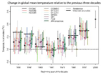
Figure 9.10. Observed and hindcast decadal mean surface temperature anomalies (°C) expressed, for each decade, relative to the preceding three decades. Observed anomalies are represented by horizontal black lines. Hindcast decadal anomalies and their uncertainties (5 to 95% confidence bounds) are displayed as vertical bars. Hindcasts are based on a Bayesian detection analysis using the estimated response to historical external forcing. Hindcasts made with CGCM2, HadCM2 (see Table 8.1 of the TAR) and HadCM3 (see Table 8.1 ,this report) use the estimated response to anthropogenic forcing only (left hand column of legend) while those made with selected MMD 20C3M models used anthropogenic and natural forcings (centre column of legend; see Table 8.1 for model descriptions). Hindcasts made with the ensemble mean of the selected 20C3M models are indicated by the thick green line. A hindcast based on persisting anomalies from the previous decade is also shown. The hindcasts agree well with observations from the 1950 s onward. Hindcasts for the decades of the 1930 s and 1940 s are sensitive to the details of the hindcast procedure. A forecast for the decadal global mean anomaly for the decade 2000 to 2009, relative to the 1970 to 1999 climatology, based on simulations performed with the Canadian Centre for Climate Modelling and Analysis Coupled Global Climate Model (CGCM2) is also displayed. From Lee et al. 2006 [JoC, MoS, SRC] ).
9.4.1.5 The Influence of Other Anthropogenic and Natural Forcings
Asignificant cooling due to other anthropogenic factors, dominated by aerosols, is a robust feature of a wide range of detection analyses. These analyses indicate that it is likely that greenhouse gases alone would have caused more than the observed warming over the last 50 years of the 20th century, with some warming offset by cooling from natural and other anthropogenic factors, notably aerosols, which have a very short residence time in the atmosphere relative to that of well-mixed greenhouse gases ( Schwartz, 1993 [ARC] ). A key factor in identifying the aerosol fingerprint, and therefore the amount of aerosol cooling counteracting greenhouse warming, is the change through time of the hemispheric temperature contrast, which is affected by the different evolution of aerosol forcing in the two hemispheres as well as the greater thermal inertia of the larger ocean area in the SH ( Santer et al., 1996b [PoC, JoC, SRC] ,c; Hegerl et al., 2001 [JoC, SRC] ; Stott et al., 2006c [JoC, MoS, SRC] ). Regional and seasonal aspects of the temperature response may help to distinguish further the response to greenhouse gas increases from the response to aerosols (e.g., Ramanathan et al., 2005 [JoC, ARC] ; Nagashima et al., 2006 [JoC] ).
Results on the importance and contribution from anthropogenic forcings other than greenhouse gases vary more between different approaches. For example, Bayesian analyses differ in the strength of evidence they find for an aerosol effect. Schnur and Hasselman 2005 [NotFound] ), for example, fail to find decisive evidence for the influence of aerosols. They postulate that this could be due to taking account of modelling uncertainty in the response to aerosols. However, two other studies using frequentist methods that also include modelling uncertainty find a clear detection of sulphate aerosols, suggesting that the use of multiple models helps to reduce uncertainties and improves detection of a sulphate aerosol effect ( Gillett et al., 2002c [NPR, JoC, MoS, SRC] ; Huntingford et al., 2006 [JoC, MoS, SRC] ). Similarly, a Bayesian study of hemispheric mean temperatures from 1900 to 1996 finds decisive evidence for an aerosol cooling effect ( Smith et al., 2003 [PoC, JoC, SRC] ). Differences in the separate detection of sulphate aerosol influences in multi-signal approaches can also reflect differences in the diagnostics applied (e.g., the space-time analysis of Tett et al. 1999 [JoC, SRC] ) versus the space-only analysis of Hegerl et al. 1997 [JoC, SRC] , 2000 )) as was shown by Gillett et al. 2002a [JoC, SRC] ).
Recent estimates( Figure 9.9 )indicate a relatively small combined effect of natural forcings on the global mean temperature evolution of the second half of the 20th century, with a small net cooling from the combined effects of solar and volcanic forcings. Coupled models simulate much less warming over the 20th century in response to solar forcing alone than to greenhouse gas forcing ( Cubasch et al., 1997 [JoC, MoS, ARC] ; Broccoli et al., 2003 [JoC, MoS, ARC] ; Meehl et al., 2004 [JoC, MoS, ARC] ), independent of which solar forcing reconstruction is used( Chapter2 ). Several studies have attempted to estimate the individual contributions from solar and volcanic forcings separately, thus allowing for the possibility of enhancement of the solar response in observations due to processes not represented in models. Optimal detection studies that attempt to separate the responses to solar and other forcings in observations can also account for gross errors in the overall magnitude of past solar forcing, which remains uncertain( Chapter2 ), by scaling the space-time patterns of response( Section 9.2.2.1 ). Using such a method, Tett et al. 1999 [JoC, SRC] ) estimate that the net anthropogenic warming in the second half of the 20th century was much greater than any possible solar warming, even when using the solar forcing reconstruction by Hoyt and Schatten 1993 [JoC] ), which indicates larger solar forcing and a different evolution over time than more recent reconstructions( Section 2.7.1 ). However, Stott et al. 2003b [JoC, MoS, SRC] ), using the same solar reconstruction but a different model, are not able to completely rule out the possibility that solar forcing might have caused more warming than greenhouse gas forcing over the 20th century due to difficulties in distinguishing between the patterns of response to solar and greenhouse forcing. This was not the case when using the response to solar forcing based on the alternative reconstruction of Lean et al. 1995 [PoC, JoC, ARC] ), in which case they find a very small likelihood (less than 1%, as opposed to approximately 10%) that solar warming could be greater than greenhouse warming since 1950 . Note that recent solar forcing reconstructions show a substantially decreased magnitude of low-frequency variations in solar forcing( Section 2.7.1 )compared to Lean et al. 1995 [PoC, JoC, ARC] ) and particularly Hoyt and Schatten 1993 [JoC] ).
The conclusion that greenhouse warming dominates over solar warming is supported further by a detection and attribution analysis using 13 models from the MMD at PCMDI ( Stone et al., 2007a [JoC, MoS, SRC, 2007] ) and an analysis of the National Center for Atmospheric Research (NCAR) Community Climate System Model (CCSM1.4; Stone et al., 2007b [JoC, SRC, 2007] ). In both these analyses, the response to solar forcing in the model was inferred by fitting a series of EBMs to the mean coupled model response to the combined effects of anthropogenic and natural forcings. In addition, a combined analysis of the response at the surface and through the depth of the atmosphere using HadCM3 and the solar reconstruction of Lean et al. 1995 [PoC, JoC, ARC] ) concluded that the near-surface temperature response to solar forcing over 1960 to 1999 is much smaller than the response to greenhouse gases ( Jones et al., 2003 [JoC, SRC] ). This conclusion is also supported by the vertical pattern of climate change, which is more consistent with the response to greenhouse gas than to solar forcing( Figure 9.1 ). Further evidence against a dominant solar role arises from older analyses targeted at detecting the solar response (e.g., North and Stevens, 1998 [JoC] ). Based on these detection results, which allow for possible amplification of the solar influence by processes not represented in climate models, we conclude that it is very likely that greenhouse gases caused more global warming over the last 50 years than changes in solar irradiance.
Detection and attribution as well as modelling studies indicate more uncertainty regarding the causes of early 20th-century warming than the recent warming. A number of studies detect a significant natural contribution to early 20th-century warming ( Tett et al., 2002 [JoC, MoS, SRC] ; Stott et al., 2003b [JoC, MoS, SRC] ; Nozawa et al., 2005 [JoC, SRC] ; Shiogama et al., 2006 [JoC] ). Some studies find a greater role for solar forcing than other forcings before 1950 ( Stott et al., 2003b [JoC, MoS, SRC] ), although one detection study finds a roughly equal role for solar and volcanic forcing ( Shiogama et al., 2006 [JoC] ), and others find that volcanic forcing ( Hegerl et al., 2003 [JoC, SRC] , 2007 ) or a substantial contribution from natural internal variability ( Tett et al., 2002 [JoC, MoS, SRC] ; Hegerl et al., 2007 [JoC, SRC, 2007] ) could be important. There could also be an early expression of greenhouse warming in the early 20th century ( Tett et al., 2002 [JoC, MoS, SRC] ; Hegerl et al., 2003 [JoC, SRC] , 2007 ).
9.4.1.6 Implications for Transient Climate Response
Quantification of the likely contributions of greenhouse gases and other forcing factors to past temperature change( Section 9.4.1.4 )in turn provides observational constraints on the transient climate response, which determines the rapidity and strength of a global temperature response to external forcing (see Glossary and Sections 9.6.2.3 and 8.6.2.1 for detailed definitions) and therefore helps to constrain likely future rates of warming. Scaling factors derived from detection analyses can be used to scale predictions of future change by assuming that the fractional error in model predictions of global mean temperature change is constant ( Allen et al., 2000 [JoC, MoS, SRC] , 2002; Allen and Stainforth, 2002 [JoC, MoS, SRC] ; Stott and Kettleborough, 2002 [JoC, MoS, SRC] ). This linear relationship between past and future fractional error in temperature change has been found to be sufficiently robust over a number of realistic forcing scenarios to introduce little additional uncertainty ( Kettleborough et al., 2007 [JoC, MoS, SRC, 2007] ). In this approach based on detection and attribution methods, which is compared with other approaches for producing probabilistic projections in Section 10.5.4.5 ,different scaling factors are applied to the greenhouse gases and to the response to other anthropogenic forcings (notably aerosols); these separate scaling factors are used to account for possible errors in the models and aerosol forcing. Uncertainties calculated in this way are likely to be more reliable than uncertainty ranges derived from simulations by coupled AOGCMs that happen to be available. Such ensembles could provide a misleading estimate of forecast uncertainty because they do not systematically explore modelling uncertainty ( Allen et al., 2002 [Ambiguous] ; Allen and Stainforth, 2002 [JoC, MoS, SRC] Stott et al. 2006c [JoC, MoS, SRC] ) compare observationally constrained predictions from three coupled climate models with a range of sensitivities and show that predictions made in this way are relatively insensitive to the particular choice of model used to produce them. The robustness to choice of model of such observationally constrained predictions was also demonstrated by Stone et al. 2007a [JoC, MoS, SRC, 2007] ) for the MMD ensemble. The observationally constrained transient climate response at the time of doubling of atmospheric CO2 following a 1% per year increase in CO2 was estimated by Stott et al. 2006c [JoC, MoS, SRC] ) to lie between 1.5°C and 2.8°C( Section 9.6.2 , Figure 9.21 ). Such approaches have also been used to provide observationally constrained predictions of global mean ( Stott and Kettleborough, 2002 [JoC, MoS, SRC] ; Stone et al., 2007a [JoC, MoS, SRC, 2007] ) and continental-scale temperatures ( Stott et al., 2006a [JoC, MoS, SRC] ) following the IPCC Special Report on Emission Scenarios (SRES) emissions scenarios, and these are discussed in Sections 10.5.4.5 and 11.10 .
Diurnal temperature range (DTR) has decreased over land by about 0.4°C over the last 50 years, with most of that change occurring prior to 1980 ( Section 3.2.2.1 ). This decreasing trend has been shown to be outside the range of natural internal variability estimated from models. Hansen et al. 1995 [ARC] ) demonstrate that tropospheric aerosols plus increases in continental cloud cover, possibly associated with aerosols, could account for the observed decrease in DTR. However, although models simulate a decrease in DTR when they include anthropogenic changes in greenhouse gases and aerosols, the observed decrease is larger than the model-simulated decrease ( Stone and Weaver, 2002 [JoC, MoS, SRC] , 2003; Braganza et al., 2004 [JoC] ). This discrepancy is associated with simulated increases in daily maximum temperature being larger than observed, and could be associated with simulated increases in cloud cover being smaller than observed ( Braganza et al., 2004 [JoC] ; see Section 3.4.3.1 for observations), a result supported by other analyses ( Dai et al., 1999 [PoC, JoC, ARC] ; Stone and Weaver, 2002 [JoC, MoS, SRC] , 2003 ).
9.4.1.7 Studies of Indices of Temperature Change
Another method for identifying fingerprints of climate change in the observational record is to use simple indices of surface air temperature patterns that reflect features of the anticipated response to anthropogenic forcing ( Karoly and Braganza, 2001 [JoC, SRC] ; Braganza et al., 2003 [JoC] ). By comparing modelled and observed changes in such indices, which include the global mean surface temperature, the land-ocean temperature contrast, the temperature contrast between the NH and SH, the mean magnitude of the annual cycle in temperature over land and the mean meridional temperature gradient in the NH mid-latitudes, Braganza et al. 2004 [JoC] ) estimate that anthropogenic forcing accounts for almost all of the warming observed between 1946 and 1995 whereas warming between 1896 and 1945 is explained by a combination of anthropogenic and natural forcing and internal variability. These results are consistent with the results from studies using space-time detection techniques( Section 9.4.1.4 ).
9.4.1.8 Remaining Uncertainties
Amuch larger range of forcing combinations and climate model simulations has been analysed in detection studies than was available for the TAR (Supplementary Material, Table S9.1). Detection and attribution analyses show robust evidence for an anthropogenic influence on climate. However, some forcings are still omitted by many models and uncertainties remain in the treatment of those forcings that are included by the majority of models.
Most studies omit two forcings that could have significant effects, particularly at regional scales, namely carbonaceous aerosols and land use changes. However, detection and attribution analyses based on climate simulations that include these forcings, (e.g., Stott et al., 2006b [JoC, MoS, SRC] ), continue to detect a significant anthropogenic influence in 20th-century temperature observations even though the near-surface patterns of response to black carbon aerosols and sulphate aerosols could be so similar at large spatial scales (although opposite in sign) that detection analyses may be unable to distinguish between them ( Jones et al., 2005 [JoC, SRC] ). Forcing from surface albedo changes due to land use change is expected to be negative globally (Sections 2.5.3 , 7.3.3 and 9.3.3.3 )although tropical deforestation could increase evaporation and warm the climate( Section 2.5.5 ), counteracting cooling from albedo change. However, the albedo-induced cooling effect is expected to be small and was not detected in observed trends in the study by Matthews et al. 2004 [JoC, ARC] ).
For those forcings that have been included in attribution analyses, uncertainties associated with the temporal and spatial pattern of the forcing and the modelled response can affect the results. Large uncertainties associated with estimates of past solar forcing( Section 2.7.1 )and omission of some chemical and dynamical response mechanisms ( Gray et al., 2005 [NPR, ARC] ) make it difficult to reliably estimate the contribution of solar forcing to warming over the 20th century. Nevertheless, as discussed above, results generally indicate that the contribution is small even if allowance is made for amplification of the response in observations, and simulations used in attribution analyses use several different estimates of solar forcing changes over the 20th century (Supplementary Material, Table S9.1). A number of different volcanic reconstructions are included in the modelling studies described in Section 9.4.1.2 (e.g., Sato et al., 1993 [JoC, ARC] ; Andronova et al., 1999 [JoC, MoS, SRC] ; Ammann et al., 2003 [PoC, JoC, MoS, SRC] ; Supplementary Material, Table S9.1). Some models include volcanic effects by simply perturbing the incoming shortwave radiation at the top of the atmosphere, while others simulate explicitly the radiative effects of the aerosols in the stratosphere. In addition, some models include the indirect effects of tropospheric sulphate aerosols on clouds (e.g., Tett et al., 2002 [JoC, MoS, SRC] ), whereas others consider only the direct radiative effect (e.g., Meehl et al., 2004 [JoC, MoS, ARC] ). In models that include indirect effects, different treatments of the indirect effect are used, including changing the albedo of clouds according to an off-line calculation (e.g., Tett et al., 2002 [JoC, MoS, SRC] ) and a fully interactive treatment of the effects of aerosols on clouds (e.g., Stott et al., 2006b [JoC, MoS, SRC] ). The overall level of consistency between attribution results derived from different models (as shown in Figure 9.9 ), and the ability of climate models to simulate large-scale temperature changes during the 20th century (Figures 9.5 and 9.6 ), indicate that such model differences are likely to have a relatively small impact on attribution results of large-scale temperature change at the surface.
There have also been methodological developments that have resulted in attribution analyses taking uncertainties more fully into account. Attribution analyses normally directly account for errors in the magnitude of the model’s pattern of response to different forcings by the inclusion of factors that scale the model responses up or down to best match observed climate changes. These scaling factors compensate for under- or overestimates of the amplitude of the model response to forcing that may result from factors such as errors in the model’s climate sensitivity, ocean heat uptake efficiency or errors in the imposed external forcing. Older analyses (e.g., Tett et al., 2002 [JoC, MoS, SRC] ) did not take account of uncertainty due to sampling signal estimates from finite-member ensembles. This can lead to a low bias, particularly for weak forcings, in the scaling factor estimates (Appendix 9.A.1; Allen and Stott, 2003 [JoC, MoS, SRC] ; Stott et al., 2003a [NPR, JoC, MoS, SRC] ). However, taking account of sampling uncertainty (as most more recent detection and attribution studies do, including those shown in Figure 9.9 )makes relatively little difference to estimates of attributable warming rates, particularly those due to greenhouse gases; the largest differences occur in estimates of upper bounds for small signals, such as the response to solar forcing ( Allen and Stott, 2003 [JoC, MoS, SRC] ; Stott et al., 2003a [NPR, JoC, MoS, SRC] ). Studies that compare results between models and analysis techniques (e.g., Hegerl et al., 2000 [JoC, MoS, SRC] ; Gillett et al., 2002a [JoC, SRC] ; Hegerl and Allen, 2002 [JoC, MoS, SRC] ), and more recently, that use multiple models to determine fingerprints of climate change ( Gillett et al., 2002c [NPR, JoC, MoS, SRC] ; Huntingford et al., 2006 [JoC, MoS, SRC] ; Stott et al., 2006c [JoC, MoS, SRC] ; Zhang et al., 2006 [JoC, MoS, SRC] ) find a robust detection of an anthropogenic signal in past temperature change.
Acommon aspect of detection analyses is that they assume the response in models to combinations of forcings to be additive. This was shown to be the case for near-surface temperatures in the PCM ( Meehl et al., 2004 [JoC, MoS, ARC] ), in the Hadley Centre Climate Model version 2 (HadCM2; Gillett et al., 2004c [JoC, MoS, SRC] ) and in the GFDL CM2.1 (see Table 8.1 )model ( Knutson et al., 2006 [JoC, MoS, ARC] ), although none of these studies considered the indirect effects of sulphate aerosols. Sexton et al. 2003 [PoC, JoC, MoS, SRC] ) did find some evidence for a nonlinear interaction between the effects of greenhouse gases and the indirect effect of sulphate aerosols in the atmosphere-only version of HadCM3 forced by observed SSTs; the additional effect of combining greenhouse gases and indirect aerosol effects together was much smaller than each term separately but was found to be comparable to the warming due to increasing tropospheric ozone. In addition, Meehl et al. 2003 [JoC, MoS, ARC] ) found that additivity does not hold so well for regional responses to solar and greenhouse forcing in the PCM. Linear additivity was found to hold in the PCM model for changes in tropopause height and synthetic satellite-borne Microwave Sounding Unit (MSU) temperatures ( Christy et al., 2000 [ARC] ; Mears et al., 2003 [JoC, ARC] ; Santer et al., 2003b [PoC, JoC, MoS, SRC] ).
Afurther source of uncertainty derives from the estimates of internal variability that are required for all detection analyses. These estimates are generally model-based because of difficulties in obtaining reliable internal variability estimates from the observational record on the spatial and temporal scales considered in detection studies. However, models would need to underestimate variability by factors of over two in their standard deviation to nullify detection of greenhouse gases in near-surface temperature data ( Tett et al., 2002 [JoC, MoS, SRC] ), which appears unlikely given the quality of agreement between models and observations at global and continental scales (Figures 9.7 and 9.8 )and agreement with inferences on temperature variability from NH temperature reconstructions of the last millennium. The detection of the effects of other forcings, including aerosols, is likely to be more sensitive (e.g., an increase of 40% in the estimate of internal variability is enough to nullify detection of aerosol and natural forcings in HadCM3; Tett et al., 2002 [JoC, MoS, SRC] )
Few detection studies have explicitly considered the influence of observational uncertainty on near-surface temperature changes. However, Hegerl et al. 2001 [JoC, SRC] ) show that inclusion of observational sampling uncertainty has relatively little effect on detection results and that random instrumental error has even less effect. Systematic instrumental errors, such as changes in measurement practices or urbanisation, could be more important, especially earlier in the record( Chapter3 ), although these errors are calculated to be relatively small at large spatial scales. Urbanisation effects appear to have negligible effects on continental and hemispheric average temperatures( Chapter3 ). Observational uncertainties are likely to be more important for surface temperature changes averaged over small regions( Section 9.4.2 )and for analyses of free atmosphere temperature changes( Section 9.4.4 ).
9.4.2 Continental and Sub-continental Surface Temperature Change
9.4.2.1 Observed Changes
Over the 1901 to 2005 period there has been warming over most of the Earth’s surface with the exception of an area south of Greenland and parts of North and South America( Figure 3.9 and Section 3.2.2.7 ,see also Figure 9.6 ). Warming has been strongest over the continental interiors of Asia and north-western North America and some mid-latitude ocean regions of the SH as well as south-eastern Brazil. Since 1979, almost all land areas with observational data coverage show warming( Figure 9.6 ). Warming is smaller in the SH than in the NH, with cooling over parts of the mid-latitude oceans. There have been widespread decreases in continental DTR since the 1950 s which coincide with increases in cloud amounts( Section 3.4.3.1 ).
9.4.2.3 Studies Based on Indices of Temperature Change and Temperature-Precipitation Relationships
Studies based on indices of temperature change support the robust detection of human influence on continental-scale land areas. Observed trends in indices of North American continental-scale temperature change, (including the regional mean, the mean land-ocean temperature contrast and the annual cycle) were found by Karoly et al. 2003 [Ambiguous] ) to be generally consistent with simulated trends under historical forcing from greenhouse gases and sulphate aerosols during the second half of the 20th century. In contrast, they find only a small likelihood of agreement with trends driven by natural forcing only during this period. An analysis of changes in Australian mean, daily maximum and daily minimum temperatures and diurnal temperature range using six coupled climate models showed that it is likely that there has been a significant contribution to observed warming in Australia from increasing greenhouse gases and sulphate aerosols ( Karoly and Braganza, 2005a [JoC, SRC] ). An anomalous warming has been found over all Australia ( Nicholls, 2003 [NPR, JoC, SRC] ) and in New South Wales ( Nicholls et al., 2005 [SRC] ) since the early 1970 s, associated with a changed relationship between annual mean maximum temperature and rainfall. Whereas interannual rainfall and temperature variations in this region are strongly inversely correlated, in recent decades temperatures have tended to be higher for a given rainfall than in previous decades. By removing the rainfall-related component of Australian temperature variations, thereby enhancing the signal-to-noise ratio, Karoly and Braganza 2005b [SRC] ) detect an anthropogenic warming signal in south-eastern Australia, although their results are affected by some uncertainty associated with their removal of rainfall-related temperature variability. A similar technique applied to the Sudan and Sahel region improved the agreement between model simulations and observations of temperature change over the last 60 years in this region ( Douville, 2006 [JoC] ) and could improve the detectability of regional temperature signals over other regions where precipitation is likely to affect the surface energy budget ( Trenberth and Shea, 2005 [PoC, JoC, ARC] ).
Observed changes in temperature extremes are consistent with the observed warming of the climate ( Alexander et al., 2006 [JoC, ARC] ) and are summarised in Section 3.8.2.1 .There has been a widespread reduction in the number of frost days in mid-latitude regions in recent decades, an increase in the number of warm extremes, particularly warm nights, and a reduction in the number of cold extremes, particularly cold nights. A number of regional studies all show patterns of changes in extremes consistent with a general warming, although the observed changes in the tails of the temperature distributions are generally not consistent with a simple shift of the entire distribution alone.
9.4.3 Surface Temperature Extremes
9.4.3.2 Global Assessments
Evidence for observed changes in short-duration extremes generally depends on the region considered and the analysis method ( IPCC, 2001 [NPR] ). Global analyses have been restricted by the limited availability of quality-controlled and homogenised daily station data. Indices of temperature extremes have been calculated from station data, including some indices from regions where daily station data are not released ( (Frich et al., 2002; ) Klein Tank and Können, 2003 [JoC] ; Alexander et al., 2006 [JoC, ARC] Kiktev et al. 2003 [PoC, JoC, MoS, SRC] ) analyse a subset of such indices by using fingerprints from atmospheric model simulations driven by prescribed SSTs. They find significant decreases in the number of frost days and increases in the number of very warm nights over much of the NH. Comparisons of observed and modelled trend estimates show that inclusion of anthropogenic effects in the model integrations improves the simulation of these changing temperature extremes, indicating that human influences are probably an important contributor to changes in the number of frost days and warm nights. Tebaldi et al. 2006 [JoC, MoS, ARC] ) find that changes simulated by eight MMD models agreed well with observed trends in heat waves, warm nights and frost days over the last four decades.
Christidis et al. 2005 [JoC] ) analyse a new gridded data set of daily temperature data ( Caesar et al., 2006 [JoC, ARC] ) using the indices shown by Hegerl et al. 2004 [JoC, SRC] ) to have a potential for attribution, namely the average temperature of the most extreme 1, 5, 10 and 30 days of the year. Christidis et al. 2005 [JoC] ) detect robust anthropogenic changes in indices of extremely warm nights using signals estimated with the HadCM3 model, although with some indications that the model overestimates the observed warming of warm nights. They also detect human influence on cold days and nights, but in this case the model underestimates the observed changes, significantly so in the case of the coldest day of the year. Anthropogenic influence was not detected in observed changes in extremely warm days.
9.4.3.3 Attributable Changes in the Risk of Extremes
Many important impacts of climate change may manifest themselves through a change in the frequency or likelihood of occurrence of extreme events. While individual extreme events cannot be attributed to external influences, a change in the probability of such events might be attributable to external influences ( Palmer, 1999 [MoS, ARC] ; Palmer and Räisänen, 2002 [JoC, ARC] ). One study estimates that anthropogenic forcings have significantly increased the risk of extremely warm summer conditions over southern Europe, as was observed during the 2003 European heat wave. Stott et al. 2004 [JoC, SRC] ) apply a methodology for making quantitative statements about change in the likelihood of such specific types of climatic events ( Allen, 2003 [JoC, SRC] ; Stone and Allen, 2005a [JoC, SRC] ), by expressing the contribution of external forcing to the risk of an event exceeding a specific magnitude. If P1 is the probability of a climatic event (such as a heat wave) occurring in the presence of anthropogenic forcing of the climate system, and P0 is the probability of it occurring if anthropogenic forcing had not been present, then the fraction of the current risk that is attributable to past greenhouse gas emissions (fraction of attributable risk; FAR) is given by FAR = 1 – P0 / P1 ( Allen, 2003 [JoC, SRC] Stott et al. 2004 [JoC, SRC] ) apply the FAR concept to mean summer temperatures of a large part of continental Europe and the Mediterranean. Using a detection and attribution analysis, they determine that regional summer mean temperature has likely increased due to anthropogenic forcing, and that the observed change is inconsistent with natural forcing. They then use the HadCM3 model to estimate the FAR associated with a particular extreme threshold of regional summer mean temperature that was exceeded in 2003, but in no other year since the beginning of the record in 1851 Stott et al. 2004 [JoC, SRC] ) estimate that it is very likely that human influence has more than doubled the risk of the regional summer mean temperature exceeding this threshold( Figure 9.13 ).
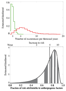
Figure 9.13. Change in risk of mean European summer temperatures exceeding a threshold of 1.6°C above 1961 to 1990 mean temperatures, a threshold that was exceeded in 2003 but in no other year since the start of the instrumental record in 1851 . (Top) Frequency histograms of the estimated likelihood of the risk (probability) of exceeding a 1.6°C threshold (relative to the 1961 – 1990 mean) in the 1990 s in the presence (red curve) and absence (green curve) of anthropogenic change, expressed as an occurrence rate. (Bottom) Fraction of attributable risk (FAR). The vertical line indicates the ‘best estimate’ FAR, the mean risk attributable to anthropogenic factors averaged over the distribution. The alternation between grey and white bands indicates the deciles of the estimated FAR distribution. The shift from the green to the red distribution in (a) implies a FAR distribution with mean 0.75, corresponding to a four-fold increase in the risk of such an event (b). From Stott et al. 2004 [JoC, SRC] ).
This study considered only continental mean seasonally averaged temperatures. Consideration of shorter-term and smaller-scale heat waves will require higher resolution modelling and will need to take complexities such as land surface processes into account ( Schär and Jendritzky, 2004 [JoC, ARC] ). Also, Stott et al. 2004 [JoC, SRC] ) assume no change in internal variability in the region they consider (which was the case in HadCM3 21st-century climate projections for summer mean temperatures in the region they consider), thereby ascribing the increase in risk only to an increase in mean temperatures (i.e., as shown in Box TS.5, Figure 1, which illustrates how a shift in the mean of a distribution can cause a large increase in the frequency of extremes). However, there is some evidence for a weak increase in European temperature variability in summer (and a decrease in winter) for the period 1961 to 2004 ( Scherrer et al., 2005 [JoC, ARC] ), which could contribute to an increase in the likelihood of extremes. Schär et al. 2004 [JoC, ARC] ) show that the central European heat wave of 2003 could also be consistent with model-predicted increases in temperature variability due to soil moisture and vegetation feedbacks. In addition, multi-decadal scale variability, associated with basin-scale changes in the Atlantic Ocean related to the Meridional Overturning Circulation (MOC) could have contributed to changes in European summer temperatures ( Sutton and Hodson, 2005 [JoC, MoS] ), although Klein Tank et al. 2005 [JoC] ) show evidence that patterns of change in European temperature variance in spring and summer are not consistent with patterns of change in temperature variance expected from natural variability. Meteorological aspects of the summer 2003 European heat wave are discussed in Box 3.6 .
9.4.4 Free Atmosphere Temperature
9.4.4.1 Observed Changes
Observed free atmosphere temperature changes are discussed in Section 3.4.1 and Karl et al. 2006 [NPR, PoC, ARC] ) provide a comprehensive review. Radiosonde-based observations (with near global coverage since 1958 ) and satellite-based temperature measurements (beginning in late 1978 ) show warming trends in the troposphere and cooling trends in the stratosphere. All data sets show that the global mean and tropical troposphere has warmed from 1958 to the present, with the warming trend in the troposphere slightly greater than at the surface. Since 1979, it is likely that there is slightly greater warming in the troposphere than at the surface, although uncertainties remain in observed tropospheric warming trends and whether these are greater or less than the surface trend. The range (due to different data sets) of the global mean tropospheric temperature trend since 1979 is 0.12°C to 0.19°C per decade based on satellite-based estimates( Chapter3 )compared to a range of 0.16°C to 0.18°C per decade for the global surface warming. While all data sets show that the stratosphere has cooled considerably from 1958 and from 1979 to present, there are large differences in the linear trends estimated from different data sets. However, a linear trend is a poor fit to the data in the stratosphere and the tropics at all levels( Section 3.4.1 ). The uncertainties in the observational records are discussed in detail in Section 3.4.1 and by Karl et al. 2006 [NPR, PoC, ARC] ). Uncertainties remain in homogenised radiosonde data sets which could result in a spurious inference of net cooling in the tropical troposphere. Differences between temperature trends measured from different versions of tropospheric satellite data result primarily from differences in how data from different satellites are merged.
9.4.4.2 Changes in Tropopause Height
The height of the lapse rate tropopause (the boundary between the stratosphere and the troposphere) is sensitive to bulk changes in the thermal structure of the stratosphere and the troposphere, and may also be affected by changes in surface temperature gradients ( Schneider, 2004 [JoC] ). Analyses of radiosonde data have documented increases in tropopause height over the past 3 to 4 decades ( Highwood et al., 2000 [JoC, ARC] ; Seidel et al., 2001 [JoC, ARC] ). Similar increases have been inferred from three different reanalysis products, the European Centre for Medium Range Weather Forecasts (ECMWF) 15- and 40-year reanalyses (ERA-15 and ERA-40) and the NCAR- National Center for Environmental Prediction (NCEP) reanalysis ( Kalnay et al., 1996 [JoC] ; Gibson et al., 1997 [NPR, MoS] ; Simmons and Gibson, 2000 [NPR, MoS, ARC] ; Kistler et al., 2001 [JoC] ), and from model simulations with combined anthropogenic and natural forcing ( Santer et al., 2003a [PoC, JoC, MoS, SRC] ,b, 2004; see Figure 9.14 ). In both models and reanalyses, changes in tropopause height over the satellite and radiosonde eras are smallest in the tropics and largest over Antarctica ( Santer et al., 2003a [PoC, JoC, MoS, SRC] ,b, 2004 ). Model simulations with individual forcings indicate that the major drivers of the model tropopause height increases are ozone-induced stratospheric cooling and the tropospheric warming caused by greenhouse gas increases ( Santer et al., 2003a [PoC, JoC, MoS, SRC] ). However, earlier model studies have found that it is difficult to alter tropopause height through stratospheric ozone changes alone ( Thuburn and Craig, 2000 [JoC] Santer et al. 2003c [PoC, JoC, SRC] ) found that the model-simulated response to combined anthropogenic and natural forcing is robustly detectable in different reanalysis products, and that solar and volcanic forcing alone could not explain the tropopause height increases( Figure 9.14 ). Climate data from reanalyses, especially the ‘first generation’ reanalysis analysed by Santer et al. 2003a [PoC, JoC, MoS, SRC] ), are subject to some deficiencies, notably inhomogeneities related to changes over time in the availability and quality of input data, and are subject to a number of specific technical choices in the reanalysis scheme (see Santer et al., 2004 [PoC, JoC, SRC] , for a discussion). Also, the NCEP reanalysis detection results could be due to compensating errors because of excessive stratospheric cooling in the reanalysis ( Santer et al., 2004 [PoC, JoC, SRC] ), since the stratosphere cools more relative to the troposphere in the NCEP reanalysis while models warm the troposphere. In contrast, the finding of a significant anthropogenic influence on tropopause height in the ‘second generation’ ERA-40 reanalysis is driven by similar large-scale changes in both models and the reanalysis. Detection results there are robust to removing global mean tropopause height increases.
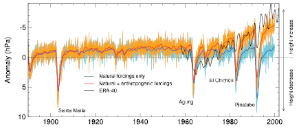
Figure 9.14. Comparison between reanalysis and climate-model simulated global monthly mean anomalies in tropopause height. Model results are from two different PCM( Table 8.1 )ensemble experiments using either natural forcings, or natural and anthropogenic forcings (ALL). There are four realisations of each experiment. Both the low-pass filtered ensemble mean and the unfiltered range between the highest and lowest values of the realisations are shown. All model anomalies are defined relative to climatological monthly means computed over 1890 to 1999 . Reanalysis-based tropopause height anomalies estimated from ERA-40 were filtered in the same way as model data. The ERA-40 record spans 1957 to 2002 and was forced to have the same mean as ALL over 1960 to 1999 . After Santer et al. 2003a [PoC, JoC, MoS, SRC] and Santer et al. 2004 [PoC, JoC, SRC] ).
9.4.4.3 Overall Atmospheric Temperature Change
Anthropogenic influence on free atmosphere temperatures has been detected in analyses of satellite data since 1979, although this finding has been found to be sensitive to which analysis of satellite data is used. Satellite-borne MSUs, beginning in 1978, estimate the temperature of thick layers of the atmosphere. The main layers represent the lower troposphere (T2LT), the mid-troposphere (T2) and the lower stratosphere (T4)( Section 3.4.1.2.1 Santer et al. 2003c [PoC, JoC, SRC] ) compare T2 and T4 temperature changes simulated by the PCM model including anthropogenic and natural forcings with the University of Alabama in Huntsville (UAH; Christy et al., 2000 [ARC] ) and Remote Sensing Systems (RSS; Mears and Wentz, 2005 [JoC, ARC] ) satellite data sets( Section 3.4.1.2.2 ). They find that the model fingerprint of the T4 response to combined anthropogenic and natural forcing is consistently detected in both satellite data sets, whereas the T2 response is detected only in the RSS data set. However, when the global mean changes are removed, the T2 fingerprint is detected in both data sets, suggesting a common spatial pattern of response overlain by a systematic global mean difference.
Anthropogenic influence on free atmosphere temperatures has been robustly detected in a number of different studies analysing various versions of the Hadley Centre Radiosonde Temperature (HadRT2) data set ( Parker et al., 1997 [JoC] ) by means of a variety of different diagnostics and fingerprints estimated with the HadCM2 and HadCM3 models ( Tett et al., 2002 [JoC, MoS, SRC] ; Thorne et al., 2002 [NPR, PoC, JoC, SRC] , 2003; Jones et al., 2003 [JoC, SRC] ). Whereas an analysis of spatial patterns of zonal mean free atmosphere temperature changes was unable to detect the response to natural forcings ( Tett et al., 2002 [JoC, MoS, SRC] ), an analysis of spatio-temporal patterns detected the influence of volcanic aerosols and (less convincingly) solar irradiance changes, in addition to detecting the effects of greenhouse gases and sulphate aerosols ( Jones et al., 2003 [JoC, SRC] ). In addition, Crooks 2004 [NPR, SRC] ) detects a solar signal in atmospheric temperature changes as seen in the HadRT2.1s radiosonde data set when a diagnostic chosen to extract the solar signal from other signals is used. The models used in these studies have poor vertical resolution in the stratosphere and they significantly underestimate stratospheric variability, thus possibly overestimating the significance of these detected signals ( Tett et al., 2002 [JoC, MoS, SRC] ). However, a sensitivity study ( Thorne et al., 2002 [NPR, PoC, JoC, SRC] ) showed that detection of human influence on free atmosphere temperature changes does not depend on the inclusion of stratospheric temperatures. An analysis of spatial patterns of temperature change, represented by large-scale area averages at the surface, in broad atmospheric layers and in lapse rates between layers, showed robust detection of an anthropogenic influence on climate when a range of uncertainties were explored relating to the choice of fingerprints and the radiosonde and model data sets ( Thorne et al., 2003 [PoC, JoC, SRC] ). However, Thorne et al. were not able to attribute recent observed tropospheric temperature changes to any particular combination of external forcing influences because the models analysed (HadCM2 and HadCM3) overestimate free atmosphere warming as estimated by the radiosonde data sets, an effect also seen by Douglass et al. 2004 [NPR, JoC, MoS] ) during the satellite era. However, there is evidence that radiosonde data during the satellite era are contaminated by spurious cooling trends ( Sherwood et al., 2005 [JoC, ARC] ; Randel and Wu, 2006 [JoC] ; Section 3.4.1 ), and since structural uncertainty arising from the choice of techniques used to analyse radiosonde data has not yet been quantified ( Thorne et al., 2005 [PoC, JoC, SRC] ), it is difficult to assess, based on these analyses alone, whether model-data discrepancies are due to model or observational deficiencies. However further information is provided by an analysis of modelled and observed tropospheric lapse rates, discussed in Section 9.4.4.4 .
Adifferent approach is to assess detectability of observed temperature changes through the depth of the atmosphere with AGCM simulations forced with observed SSTs, although the vertical profile of the atmospheric temperature change signal estimated in this way can be quite different from the same signal estimated by coupled models with the same external forcings ( Hansen et al., 2002 [JoC, MoS, ARC] ; Sun and Hansen, 2003 [JoC, MoS, ARC] ; Santer et al., 2005 [PoC, JoC, SRC] Sexton et al. 2001 [JoC, SRC] ) find that inclusion of anthropogenic effects improves the simulation of zonally averaged upper air temperature changes from the HadRTt1.2 data set such that an anthropogenic signal is detected at the 5% significance level in patterns of seasonal mean temperature change calculated as overlapping eight-year means over the 1976 to 1994 period and expressed as anomalies relative to the 1961 to 1975 base period. In addition, analysing patterns of annual mean temperature change for individual years shows that an anthropogenic signal is also detected on interannual time scales for a number of years towards the end of the analysis period.
9.4.4.4 Differential Temperature Trends
Subtracting temperature trends at the surface from those in the free atmosphere removes much of the common variability between these layers and tests whether the model-predicted trends in tropospheric lapse rate are consistent with those observed by radiosondes and satellites ( Karl et al., 2006 [NPR, PoC, ARC] ). Since 1979, globally averaged modelled trends in tropospheric lapse rates are consistent with those observed. However, this is not the case in the tropics, where most models have more warming aloft than at the surface while most observational estimates show more warming at the surface than in the troposphere ( Karl et al., 2006 [NPR, PoC, ARC] Karl et al. 2006 [NPR, PoC, ARC] ) carried out a systematic review of this issue. There is greater consistency between simulated and observed differential warming in the tropics in some satellite measurements of tropospheric temperature change, particularly when the effect of the cooling stratosphere on tropospheric retrievals is taken into account ( Karl et al., 2006 [NPR, PoC, ARC] ). External forcing other than greenhouse gas changes can also help to reconcile some of the differential warming, since both volcanic eruptions and stratospheric ozone depletion are expected to have cooled the troposphere more than the surface over the last several decades ( Santer et al., 2000 [PoC, JoC, SRC] , 2001; IPCC, 2001 [NPR] ; Free and Angell, 2002 [NPR, JoC, ARC] ; Karl et al., 2006 [NPR, PoC, ARC] ). There are, however, uncertainties in quantifying the differential cooling caused by these forcings, both in models and observations, arising from uncertainties in the forcings and model response to the forcings. Differential effects of natural modes of variability, such as ENSO and the NAM, on observed surface and tropospheric temperatures, which arise from differences in the amplitudes and spatial expression of these modes at the surface and in the troposphere, make only minor contributions to the overall differences in observed surface and tropospheric warming rates ( Santer et al., 2001 [PoC, JoC, MoS, SRC] ; Hegerl and Wallace, 2002 [JoC, SRC] ; Karl et al., 2006 [NPR, PoC, ARC] ).
Asystematic intercomparison between radiosonde-based (Radiosonde Atmospheric Temperature Products for Assessing Climate (RATPAC); Free et al., 2005 [JoC, ARC] , and Hadley Centre Atmospheric Temperature (HadAT), Thorne et al., 2005 [PoC, JoC, SRC] ) and satellite-based (RSS, UAH) observational estimates of tropical lapse rate trends with those simulated by 19 MMD models shows that on monthly and annual time scales, variations in temperature at the surface are amplified aloft in both models and observations by consistent amounts ( Santer et al., 2005 [PoC, JoC, SRC] ; Karl et al., 2006 [NPR, PoC, ARC] ). It is only on longer time scales that disagreement between modelled and observed lapse rates arises ( Hegerl and Wallace, 2002 [JoC, SRC] ), that is, on the time scales over which discrepancies would arise from inhomogeneities in the observational record. Only one observational data set (RSS) was found to be consistent with the models on both short and long time scales. While Vinnikov et al. 2006 [JoC] ) have not produced a lower-tropospheric retrieval, their estimate of the T2 temperature trend( Figure 3.18 )is consistent with model simulations ( Karl et al., 2006 [NPR, PoC, ARC] ). One possibility is that amplification effects are controlled by different physical mechanisms on short and long time scales, although a more probable explanation is that some observational records are contaminated by errors that affect their long-term trends( Section 3.4.1 ;Karl et al., 2006 [NPR, PoC, ARC] ).
9.4.5 Summary
Since the TAR, the evidence has strengthened that human influence has increased global temperatures near the surface of the Earth. Every year since the publication of the TAR has been in the top ten warmest years in the instrumental global record of near-surface temperatures. Many climate models are now available which simulate global mean temperature changes that are consistent with those observed over the last century when they include the most important forcings of the climate system. The fact that no coupled model simulation so far has reproduced global temperature changes over the 20th century without anthropogenic forcing is strong evidence for the influence of humans on global climate. This conclusion is robust to variations in model formulation and uncertainties in forcings as far as they have been explored in the large multi-model ensemble now available( Figure 9.5 ).
Many studies have detected a human influence on near-surface temperature changes, applying a variety of statistical techniques and using many different climate simulations. Comparison with observations shows that the models used in these studies appear to have an adequate representation of internal variability on the decadal to inter-decadal time scales important for detection( Figure 9.7 ). When evaluated in a Bayesian framework, very strong evidence is found for a human influence on global temperature change regardless of the choice of prior distribution.
Since the TAR, there has been an increased emphasis on partitioning the observed warming into contributions from greenhouse gas increases and other anthropogenic and natural factors. These studies lead to the conclusion that greenhouse gas forcing has very likely been the dominant cause of the observed global warming over the last 50 years, and account for the possibility that the agreement between simulated and observed temperature changes could be reproduced by different combinations of external forcing. This is because, in addition to detecting the presence of model-simulated spatio-temporal response patterns in observations, such analyses also require consistency between the model-simulated and observational amplitudes of these patterns.
Detection and attribution analyses indicate that over the past century there has likely been a cooling influence from aerosols and natural forcings counteracting some of the warming influence of the increasing concentrations of greenhouse gases( Figure 9.9 ). Spatial information is required in addition to temporal information to reliably detect the influence of aerosols and distinguish them from the influence of increased greenhouse gases. In particular, aerosols are expected to cause differential warming and cooling rates between the NH and SH that change with time depending on the evolution of the aerosol forcing, and this spatio-temporal fingerprint can help to constrain the possible range of cooling from aerosols over the century. Despite continuing uncertainties in aerosol forcing and the climate response, it is likely that greenhouse gases alone would have caused more warming than observed during the last 50 years, with some warming offset by cooling from aerosols and other natural and anthropogenic factors. The overall evidence from studies using instrumental surface temperature and free atmospheric temperature data, along with evidence from analysis of temperature over the last few hundred years( Section 9.3.3.2 ), indicates that it is very unlikely that the contribution from solar forcing to the warming of the last 50 years was larger than that from greenhouse gas forcing.
An important development since the TAR has been the detection of an anthropogenic signal in surface temperature changes since 1950 over continental and sub-continental scale land areas. The ability of models to simulate many aspects of the temperature evolution at these scales( Figure 9.12 )and the detection of significant anthropogenic effects on each of six continents provides stronger evidence of human influence on the global climate than was available to the TAR. Difficulties remain in attributing temperature changes at smaller than continental scales and over time scales of less than 50 years. Attribution at these scales has, with limited exceptions, not yet been established. Temperature changes associated with some modes of variability, which could be wholly or partly naturally caused, are poorly simulated by models in some regions and seasons and could be confounded with the expected temperature response to external forcings. Averaging over smaller regions reduces the natural variability less than averaging over large regions, making it more difficult to distinguish changes expected from external forcing. In addition, the small-scale details of external forcing and the response simulated by models are less credible than large-scale features. Overall, uncertainties in observed and model-simulated climate variability and change at smaller spatial scales make it difficult at present to estimate the contribution of anthropogenic forcing to temperature changes at scales smaller than continental and on time scales shorter than 50 years.
There is now some evidence that anthropogenic forcing has affected extreme temperatures. There has been a significant decrease in the frequency of frost days and an increase in the incidence of warm nights. A detection and attribution analysis has shown a significant human influence on patterns of changes in extremely warm nights and evidence for a human-induced warming of the coldest nights and days of the year. Many important impacts of climate change are likely to manifest themselves through an increase in the frequency of heat waves in some regions and a decrease in the frequency of extremely cold events in others. Based on a single study, and assuming a model-based estimate of temperature variability, past human influence may have more than doubled the risk of European mean summer temperatures as high as those recorded in 2003 ( Figure 9.13 ).
Since the TAR, further evidence has accumulated that there has been a significant anthropogenic influence on free atmosphere temperature since widespread measurements became available from radiosondes in the late 1950 s. The influence of greenhouse gases on tropospheric temperatures has been detected, as has the influence of stratospheric ozone depletion on stratospheric temperatures. The combination of a warming troposphere and a cooling stratosphere has likely led to an increase in the height of the tropopause and model-data comparisons show that greenhouse gases and stratospheric ozone changes are likely largely responsible( Figure 9.14 ).
Whereas, on monthly and annual time scales, variations of temperature in the tropics at the surface are amplified aloft in both the MMD simulations and observations by consistent amounts, on longer time scales, simulations of differential tropical warming rates between the surface and the free atmosphere are inconsistent with some observational records. One possible explanation for the discrepancies on multi-annual but not shorter time scales is that amplification effects are controlled by different physical mechanisms, but a more probable explanation is that some observational records are contaminated by errors that affect their long-term trends.
9.5 Understanding of Change in Other Variables during the Industrial Era
The objective of this section is to assess large-scale climate change in variables other than air temperature, including changes in ocean climate, atmospheric circulation, precipitation, the cryosphere and sea level. This section draws heavily on Chapters 3 , 4 , 5 and 8 .Where possible, it attempts to identify links between changes in different variables, such as those that associate some aspects of SST change with precipitation change. It also discusses the role of external forcing, drawing where possible on formal detection studies.
9.5.1 Ocean Climate Change
9.5.1.1 Ocean Heat Content Changes
Since the TAR, evidence of climate change has accumulated within the ocean, both at regional and global scales( Chapter5 ). The overall heat content in the World Ocean is estimated to have increased by 14.2 × 10²² J during the period 1961 to 2003 ( Section 5.2.2 ). This overall increase has been superimposed on strong interannual and inter-decadal variations. The fact that the entire ocean, which is by far the system’s largest heat reservoir ( Levitus et al., 2005 [JoC, ARC] ; see also Figure 5.4 )gained heat during the latter half of the 20th century is consistent with a net positive radiative forcing of the climate system. Late 20th-century ocean heat content changes were at least one order of magnitude larger than the increase in energy content of any other component of the Earth’s ocean-atmosphere-cryosphere system( Figure 5.4 ;Levitus et al., 2005 [JoC, ARC] ).
All analyses indicate a large anthropogenic component of the positive trend in global ocean heat content. Levitus et al. 2001 [JoC, ARC] and Gregory et al 2004 [JoC, MoS, SRC] ) analyse simulations from the GFDL R30 and HadCM3 models respectively and show that climate simulations agree best with observed changes when the models include anthropogenic forcings from increasing greenhouse gas concentrations and sulphate aerosols. Gent and Danabasoglu 2004 [JoC, MoS, ARC] ) show that the observed trend cannot be explained by natural internal variability as simulated by a long control run of the Community Climate System Model (CCSM2). Barnett et al. 2001 [JoC, SRC] and Reichert et al. 2002b [JoC, MoS] ) use detection analyses similar to those described in Section 9.4 to detect model-simulated ocean climate change signals in the observed spatio-temporal patterns of ocean heat content across the ocean basins.
Barnett et al. 2005 [JoC] ) extend previous detection and attribution analyses of ocean heat content changes to a basin by basin analysis of the temporal evolution of temperature changes in the upper 700 m of the ocean (see also Pierce et al., 2006 [JoC, MoS, SRC] ). They report that whereas the observed change is not consistent with internal variability and the response to natural external forcing as simulated by two climate models (PCM and HadCM3), the simulated ocean warming due to anthropogenic factors (including well-mixed greenhouse gases and sulphate aerosols) is consistent with the observed changes and reproduces many of the different responses seen in the individual ocean basins( Figure 9.15 ), indicating a human-induced warming of the world’s oceans with a complex vertical and geographical structure that is simulated quite well by the two AOGCMs. Barnett et al. 2005 [JoC] ) find that the earlier conclusions of Barnett et al. 2001 [JoC, SRC] ) were not affected by the Levitus et al. 2005 [JoC, ARC] ) revisions to the Levitus et al. 2000 [JoC, ARC] ) ocean heat content data.
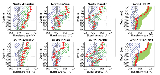
Figure 9.15. Strength of observed and model-simulated warming signal by depth for the World Ocean and for each ocean basin individually (in oC, see Barnett et al., 2005 [JoC] and Pierce et al., 2006 [JoC, MoS, SRC] for calculation of signal strength). For ocean basins, the signal is estimated from PCM( Table 8.1 )while for the World Ocean it is estimated from both PCM and HadCM3( Table 8.1 ). Red dots represent the projection of the observed temperature changes onto the normalised model-based pattern of warming. They show substantial basin-to-basin differences in how the oceans have warmed over the past 40 years, although all oceans have experienced net warming over that interval. The red bars represent the ±2 standard deviation limits associated with sampling uncertainty. The blue crosshatched swaths represent the 90% confidence limits of the natural internal variability strength. The green crosshatched swaths represent the range of the anthropogenically forced signal estimates from different realisations of identically forced simulations with the PCM model for each ocean basin (the smaller dots within the green swaths are the individual realisations) and the green shaded regions represent the range of anthropogenically forced signal estimates from different realisations of identically forced simulations with the PCM and HadCM3 models for the World Ocean (note that PCM and HadCM3 use different representations of anthropogenic forcing). The ensemble-averaged strength of the warming signal in four PCM simulations with solar and volcanic forcing is also shown (grey triangles). From Barnett et al. 2005 [JoC] and Pierce et al. 2006 [JoC, MoS, SRC] ).
In contrast, changes in solar forcing can potentially explain only a small fraction of the observationally based estimates of the increase in ocean heat content ( Crowley et al., 2003 [PoC, JoC, MoS] ), and the cooling influence of natural (volcanic) and anthropogenic aerosols would have slowed ocean warming over the last half century. Delworth et al. 2005 [JoC, MoS, SRC] ) find a delay of several decades and a reduction in the magnitude of the warming of approximately two-thirds in simulations with the GFDL-CM2 model that included these forcings compared to the response to increasing greenhouse gases alone, consistent with results based on an upwelling diffusion EBM ( Crowley et al., 2003 [PoC, JoC, MoS] ). Reductions in ocean heat content are found following volcanic eruptions in climate simulations ( Church et al., 2005 [JoC, ARC] ), including a persistent centennial time-scale signal of ocean cooling at depth following the eruption of Krakatoa ( Gleckler et al., 2006 [JoC, ARC] ).
Although the heat uptake in the ocean cannot be explained without invoking anthropogenic forcing, there is some evidence that the models have overestimated how rapidly heat has penetrated below the ocean’s mixed layer ( Forest et al., 2006 [JoC, MoS, ARC] ; see also Figure 9.15 ). In simulations that include natural forcings in addition to anthropogenic forcings, eight coupled climate models simulate heat uptake of 0.26 ± 0.06 Wm–2 (±1 standard deviation) for 1961 to 2003, whereas observations of ocean temperature changes indicate a heat uptake of 0.21 ± 0.04 Wm–2 ( Section 5.2.2.1 ). These could be consistent within their uncertainties but might indicate a tendency of climate models to overestimate ocean heat uptake.
In addition, the interannual to decadal variability seen in Levitus et al. 2000 [JoC, ARC] , 2005 )( Section 5.2.2 )is underestimated by models; Gregory et al. 2004 [JoC, MoS, SRC] ) show significant differences between observed and modelled interannual deviations from a linear trend in five-year running means of world ocean heat content above 3,000 m for 1957 to 1994 . While some studies note the potential importance of the choice of infilling method in poorly sampled regions ( Gregory et al., 2004 [JoC, MoS, SRC] ; AchutaRao et al., 2006 [JoC, MoS, ARC] ), the consistency of the differently processed data from the Levitus et al. 2005 [JoC, ARC] Ishii et al. 2006 [MoS, ARC] and Willis et al. 2004 [JoC, ARC] ) analyses adds confidence to their use for analysing trends in climate change studies( Chapter5 Gregory et al. 2004 [JoC, MoS, SRC] ) show that agreement between models and observations is better in the well-observed upper ocean (above 300 m) in the NH and that there is large sensitivity to the method of infilling the observational data set outside this well-observed region. They find a strong maximum in variability in the Levitus data set at around 500 m depth that is not seen in HadCM3 simulations, a possible indication of model deficiency or an artefact in the Levitus data. AchutaRao et al. 2006 [JoC, MoS, ARC] ) also find that observational estimates of temperature variability over much of the oceans may be substantially affected by sparse observational coverage and the method of infilling.
9.5.1.2 Water Mass Properties
Interior water masses, which are directly ventilated at the ocean surface, act to integrate highly variable surface changes in heat and freshwater, and could therefore provide indicators of global change ( Stark et al., 2006 [JoC, SRC] ). Some studies have attempted to investigate changes in three-dimensional water mass properties( Section 5.3 ). Sub-Antarctic Mode Water (SAMW) and the subtropical gyres have warmed in the Indian and Pacific basins since the 1960 s, waters at high latitudes have freshened in the upper 500 m and salinity has increased in some of the subtropical gyres. These changes are consistent with an increase in meridional moisture flux over the oceans over the last 50 years leading to increased precipitation at high latitudes( Section 5.2.3 ;Wong et al., 1999 [JoC, ARC] ) and a reduction in the difference between precipitation and evaporation at mid-latitudes( Section 5.6 ). This suggests that the ocean might integrate rainfall changes to produce detectable salinity changes. Boyer et al. 2005 [JoC, ARC] ) estimated linear trends in salinity for the global ocean from 1955 to 1998 that indicate salinification in the Antarctic Polar Frontal Zone around 40°S and in the subtropical North Atlantic, and freshening in the sub-polar Atlantic (Figures 5.5 and 5.7 ). However, variations in other terms (e.g., ocean freshwater transport) may be contributing substantially to the observed salinity changes and have not been quantified.
An observed freshening of SAMW in the South Indian Ocean between the 1960 s and 1990 s has been shown to be consistent with anthropogenically forced simulations from HadCM3 ( Banks et al., 2000 [JoC] ) but care should be taken in interpreting sparse hydrographic data, since apparent trends could reflect natural variability or the aliased effect of changing observational coverage. Although SAMW was fresher along isopycnals in 1987 than in the 1960 s, in 2002 the salinity was again near the 1960 s values ( Bindoff and McDougall, 2000 [ARC] ; Bryden et al., 2003 [JoC, ARC] ). An analysis of an ocean model forced by observed atmospheric fluxes and SSTs indicates that this is likely associated with natural variability ( Murray et al., 2007 [NPR, JoC, MoS, ARC, 2007] ), a result supported by an analysis of 20th-century simulations with HadCM3 which shows that it is not possible to reject the null hypothesis that the observed differences are due to internal variability ( Stark et al., 2006 [JoC, SRC] ), although this model does project a long-term freshening trend in the 21st century due to the large-scale response to surface heating and hydrological changes ( Banks et al., 2000 [JoC] ).
9.5.1.3 Changes in the Meridional Overturning Circulation
It is possible that anthropogenic and natural forcing may have influenced the MOC in the Atlantic (see also Box 5.1 ). One possible oceanic consequence of climate change is a slowing down or even halting of the MOC. An estimate of the overturning circulation and associated heat transport based on a trans-Atlantic section along latitude 25°N indicates that the Atlantic MOC has slowed by about 30% over five samples taken between 1957 and 2004 ( Bryden et al., 2005 [JoC] ), although given the infrequent sampling and considerable variability it is not clear whether the trend estimate is robust( Box 5.1 ). Freshening of North East Atlantic Deep Water has been observed ( Dickson et al., 2002 [JoC] ; Curry et al., 2003 [JoC, ARC] ; Figure 5.6 )and has been interpreted as being consistent with an enhanced difference between precipitation and evaporation at high latitudes and a possible slowing down of the MOC. Wu et al. 2004 [NPR, JoC, SRC] ) show that the observed freshening trend is well reproduced by an ensemble of HadCM3 simulations that includes both anthropogenic and natural forcings, but this freshening coincides with a strengthening rather than a weakening trend in the MOC. Therefore, this analysis is not consistent with an interpretation of the observed freshening trends in the North Atlantic as an early signal of a slowdown of the thermohaline circulation. Dickson et al. 2002 [JoC] ) propose a possible role for the Arctic in driving the observed freshening of the subpolar North Atlantic. Wu et al. 2005 [JoC, SRC] ) show that observed increases in arctic river flow ( Peterson et al., 2002 [JoC] ) are well simulated by HadCM3 including anthropogenic and natural forcings and propose that this increase is anthropogenic, since it is not seen in HadCM3 simulations including just natural forcing factors. However, the relationship between this increased source of freshwater and freshening in the Labrador Sea is not clear in the HadCM3 simulations, since Wu et al. 2007 [NPR, MoS, SRC, 2007] ) find that recent freshening in the Labrador Sea is simulated by the model when it is driven by natural rather than anthropogenic forcings. Importantly, freshening is also associated with decadal and multi-decadal variability, with links to the NAO( Box 5.1 )and the AMO( Box 5.1 ;Vellinga and Wu, 2004 [JoC] ; Knight et al., 2005 [JoC] ).
9.5.2 Sea Level
Aprecondition for attributing changes in sea level rise to anthropogenic forcing is that model-based estimates of historical global mean sea level rise should be consistent with observational estimates. Although AOGCM simulations of global mean surface air temperature trends are generally consistent with observations( Section 9.4.1 , Figure 9.5 ), consistency with surface air temperature alone does not guarantee a realistic simulation of thermal expansion, as there may be compensating errors among climate sensitivity, ocean heat uptake and radiative forcing (see, e.g., Raper et al., 2002 [JoC, SRC] , see also Section 9.6 ). Model simulations also offer the possibility of attributing past sea level changes to particular forcing factors. The observational budget for sea level( Section 5.5.6 )assesses the periods 1961 to 2003 and 1993 to 2003 . Table 9.2 evaluates the same terms from 20C3M simulations in the MMD at PCMDI, although most 20C3M simulations end earlier (between 1999 and 2002 ), so the comparison is not quite exact.
Table 9.2. Components of the rate of global mean sea level rise (mm yr–1)from models and observations. All ranges are 5 to 95% confidence intervals. The observational components and the observed rate of sea level rise (‘Obs’ column) are repeated from Section 5.5.6 and Table 5.3. The ‘ALL’ column is computed (following the methods of Gregory and Huybrechts, 2006 [JoC, MoS, SRC] and Section 10.6.3.1 )from eight 20C3M simulations that include both natural and anthropogenic forcings (models 3, 9, 11, 12, 14, 15, 19 and 21; see Table 8.1), and the ‘ALL/ANT’ column from 16 simulations: the eight ALL and eight others that have anthropogenic forcings only (models 4, 6, 7, 8, 13, 16, 20 and 22; see Table 8.1).
| 1961–2003 | 1993–2003 | |||||
|---|---|---|---|---|---|---|
| Obs | ALL | ALL/ANT | Obs | ALL | ALL/ANT | |
| Thermal expansion | 0.42 ± 0.12 | 0.5 ± 0.2 | 0.7 ± 0.4 | 1.60 ± 0.50 | 1.5 ± 0.7 | 1.2 ± 0.9 |
| Glaciers and ice caps | 0.50 ± 0.18 | 0.5 ± 0.2 | 0.5 ± 0.3 | 0.77 ± 0.22 | 0.7 ± 0.3 | 0.8 ± 0.3 |
| Ice sheets (observed) | 0.19 ± 0.43 | 0.41 ± 0.35 | ||||
| Sum of components | 1.1 ± 0.5 | 1.2 ± 0.5 | 1.4 ± 0.7 | 2.8 ± 0.7 | 2.6 ± 0.8 | 2.4 ± 1.0 |
| Observed rate of rise | 1.8 ± 0.5 | 3.1 ± 0.7 | ||||
Simulations including natural as well as anthropogenic forcings (the ‘ALL’ models in Table 9.2 )generally have smaller ocean heat uptake during the period 1961 to 2003 than those without volcanic forcing, since several large volcanic eruptions cooled the climate during this period ( Gleckler et al., 2006 [JoC, ARC] ). This leads to a better agreement of those simulations with thermal expansion estimates based on observed ocean warming( Section 5.5.3 )than for the complete set of model simulations (‘ALL/ANT’ in Table 9.2 ). For 1993 to 2003, the models that include natural forcings agree well with observations. Although this result is somewhat uncertain because the simulations end at various dates from 1999 onwards, it accords with results obtained by Church et al. 2005 [JoC, ARC] ) using the PCM and Gregory et al. 2006 [Ambiguous] ) using HadCM3, which suggest that 0.5 mm yr–1 of the trend in the last decade may result from warming as a recovery from the Mt. Pinatubo eruption of 1991 . Comparison of the results for 1961 to 2003 and 1993 to 2003 shows that volcanoes influence the ocean differently over shorter and longer periods. The rapid expansion of 1993 to 2003 was caused, in part, by rapid warming of the upper ocean following the cooling due to the Mt. Pinatubo eruption, whereas the multi-decadal response is affected by the much longer persistence in the deep ocean of cool anomalies caused by volcanic eruptions ( Delworth et al., 2005 [JoC, MoS, SRC] ; Gleckler et al., 2006 [JoC, ARC] ; Gregory et al., 2006 [Ambiguous] ).
Both observations and model results indicate that the global average mass balance of glaciers and ice caps depends linearly on global average temperature change, but observations of accelerated mass loss in recent years suggest a greater sensitivity than simulated by models. The global average temperature change simulated by AOGCMs gives a good match to the observational estimates of the contribution of glaciers and ice caps to sea level change in 1961 to 2003 and 1993 to 2003 ( Table 9.2 )with the assumptions that the global average mass balance sensitivity is 0.80 mm yr–1 °C–1 (sea level equivalent) and that the climate of 1900 to 1929 was 0.16°C warmer than the temperature required to maintain the steady state for glaciers (see discussion in Section 10.6.3.1 and Appendix 10.A).
Calculations of ice sheet surface mass balance changes due to climate change (following the methods of Gregory and Huybrechts, 2006 [JoC, MoS, SRC] and Section 10.6.3.1 )indicate small but uncertain contributions during 1993 to 2003 of 0.1 ± 0.1 mm yr–1 (5 to 95% range) from Greenland and –0.2 ± 0.4 mm yr–1 from Antarctica, the latter being negative because rising temperature in AOGCM simulations leads to greater snow accumulation (but negligible melting) at present. The observational estimates (Sections 4.6.2 and 5.5.6 )are 0.21 ± 0.07 mm yr–1 for Greenland and 0.21 ± 0.35 mm yr–1 for Antarctica. For both ice sheets, there is a significant contribution from recent accelerations in ice flow leading to greater discharge of ice into the sea, an effect that is not included in the models because its causes and mechanisms are not yet properly understood (see Sections 4.6.2 and 10.6.4 for discussion). Hence, the surface mass balance model underestimates the sea level contribution from ice sheet melting. Model-based and observational estimates may also differ because the model-based estimates are obtained using estimates of the correlation between global mean climate change and local climate change over the ice sheets in the 21st century under SRES scenarios. This relationship may not represent recent changes over the ice sheets.
Summing the modelled thermal expansion, global glacier and ice cap contributions and the observational estimates of the ice sheet contributions results in totals that lie below the observed rates of global mean sea level rise during 1961 to 2003 and 1993 to 2003 . As shown by Table 9.2 ,the terms are reasonably well reproduced by the models. Nevertheless, the discrepancy in the total, especially for 1961 to 2003, indicates the lack of a satisfactory explanation of sea level rise. This is also a difficulty for the observational budget (discussed in Section 5.5.6 ).
Adiscrepancy between model and observations could also be partly explained by the internally generated variability of the climate system, which control simulations suggest could give a standard deviation in the thermal expansion component of ~0.2 mm yr–1 in 10-year trends. This variability may be underestimated by models, since observations give a standard deviation in 10-year trends of 0.7 mm yr–1 in thermal expansion (see Sections 5.5.3 and Section 9.5.1.1 ;Gregory et al., 2006 [Ambiguous] ).
Since recent warming and thermal expansion are likely largely anthropogenic( Section 9.5.1.1 ), the model results suggest that the greater rate of rise in 1993 to 2003 than in 1961 to 2003 could have been caused by rising anthropogenic forcing. However, tide gauge estimates suggests larger variability than models in 10-year trends, and that rates as large as that observed during 1993 to 2003 occurred in previous decades( Section 5.5.2.4 ).
Overall, it is very likely that the response to anthropogenic forcing contributed to sea level rise during the latter half of the 20th century. Models including anthropogenic and natural forcing simulate the observed thermal expansion since 1961 reasonably well. Anthropogenic forcing dominates the surface temperature change simulated by models, and has likely contributed to the observed warming of the upper ocean and widespread glacier retreat. It is very unlikely that the warming during the past half century is due only to known natural causes. Lack of studies quantifying the contribution of anthropogenic forcing to ocean heat content increase and glacier melting, and the fact that the observational budget is not closed, make it difficult to estimate the anthropogenic contribution. Nevertheless, an expert assessment based on modelling and ocean heat content studies suggests that anthropogenic forcing has likely contributed at least one-quarter to one-half of the sea level rise during the second half of the 20th century (see also Woodworth et al., 2004 [NPR, SRC] ).
Anthropogenic forcing is also expected to produce an accelerating rate of sea level rise ( Woodworth et al., 2004 [NPR, SRC] ). On the other hand, natural forcings could have increased the rate of sea level rise in the early 20th century and decreased it later in the 20th century, thus producing a steadier rate of rise during the 20th century when combined with anthropogenic forcing ( Crowley et al., 2003 [PoC, JoC, MoS] ; Gregory et al., 2006 [Ambiguous] ). Observational evidence for acceleration during the 20th century is equivocal, but the rate of sea level rise was greater in the 20th than in the 19th century( Section 5.5.2.4 ). An onset of higher rates of rise in the early 19th century could have been caused by natural factors, in particular the recovery from the Tambora eruption of 1815 ( Crowley et al., 2003 [PoC, JoC, MoS] ; Gregory et al., 2006 [Ambiguous] ), with anthropogenic forcing becoming important later in the 19th century.
9.5.3 Atmospheric Circulation Changes
Natural low-frequency variability of the climate system is dominated by a small number of large-scale circulation patterns such as ENSO, the Pacific Decadal Oscillation (PDO), and the NAM and Southern Annular Mode (SAM)( Section 3.6 and Box 3.4 ). The impact of these modes on terrestrial climate on annual to decadal time scales can be profound, but the extent to which they can be excited or altered by external forcing remains uncertain. While some modes might be expected to change as a result of anthropogenic effects such as the enhanced greenhouse effect, there is little apriori expectation about the direction or magnitude of such changes.
9.5.3.1 El Niño-Southern Oscillation/Pacific Decadal Oscillation
The El Niño-Southern Oscillation is the leading mode of variability in the tropical Pacific, and it has impacts on climate around the globe( Section 3.6.2 ). There have been multi-decadal oscillations in the ENSO index (conventionally defined as a mean SST anomaly in the eastern equatorial Pacific) throughout the 20th century, with more intense El Niño events since the late 1970 s, which may reflect in part a mean warming of the eastern equatorial Pacific ( Mendelssohn et al., 2005 [JoC] ). Model projections of future climate change generally show a mean state shift towards more El-Niño-like conditions, with enhanced warming in the eastern tropical Pacific and a weakened Walker Circulation( Section 10.3.5.3 ); there is some evidence that such a weakening has been observed over the past 140 years ( Vecchi et al., 2006 [JoC, MoS] ). While some simulations of the response to anthropogenic influence have shown an increase in ENSO variability in response to greenhouse gas increases ( Timmermann, 1999 [Ambiguous] ; Timmermann et al., 1999 [Ambiguous] ; Collins, 2000b [JoC, ARC] ), others have shown no change (e.g., Collins, 2000a [JoC, MoS, ARC] ) or a decrease in variability ( Knutson et al., 1997 [JoC, MoS, ARC] ). A recent survey of the simulated response to atmospheric CO2 doubling in 15 MMD AOGCMs ( Merryfield, 2006 [JoC, MoS] ) finds that three of the models exhibited significant increases in ENSO variability, five exhibited significant decreases and seven exhibited no significant change. Thus, as yet there is no detectable change in ENSO variability in the observations, and no consistent picture of how it might be expected to change in response to anthropogenic forcing( Section 10.3.5.3 ).
Decadal variability in the North Pacific is characterised by variations in the strength of the Aleutian Low coupled to changes in North Pacific SST (Sections 3.6.3 and 8.4.2 ). The leading mode of decadal variability in the North Pacific is usually referred to as the PDO, and has a spatial structure in the atmosphere and upper North Pacific Ocean similar to the pattern that is associated with ENSO. One recent study showed a consistent tendency towards the positive phase of the PDO in observations and simulations with the MIROC model that included anthropogenic forcing ( Shiogama et al., 2005 [JoC, MoS, SRC] ), although differences between the observed and simulated PDO patterns, and the lack of additional studies, limit confidence in these findings.
9.5.3.2 North Atlantic Oscillation/Northern Annular Mode
The NAM is an approximately zonally symmetric mode of variability in the NH ( Thompson and Wallace, 1998 [JoC] ), and the NAO ( Hurrell, 1996 [JoC, ARC] ) may be viewed as its Atlantic counterpart( Section 3.6.4 ). The NAM index exhibited a pronounced trend towards its positive phase between the 1960 s and the 1990 s, corresponding to a decrease in surface pressure over the Arctic and an increase over the subtropical North Atlantic (see Section 3.6.4 ;see also Hurrell, 1996 [JoC, ARC] ; Thompson et al., 2000 [Ambiguous] ; Gillett et al., 2003a [NPR, PoC, SRC] ). Several studies have shown this trend to be inconsistent with simulated internal variability ( Osborn et al., 1999 [PoC, JoC, MoS, ARC] ; Gillett et al., 2000 [JoC, SRC] , 2002b; Osborn, 2004 [PoC, JoC, MoS, ARC] ; Gillett, 2005 [JoC, SRC] ). Although the NAM index has decreased somewhat since its peak in the mid- 1990 s, the trend calculated over recent decades remains significant at the 5% significance level compared to simulated internal variability in most models ( Osborn, 2004 [PoC, JoC, MoS, ARC] ; Gillett, 2005 [JoC, SRC] ), although one study found that the NAO index trend was marginally consistent with internal variability in one model ( Selten et al., 2004 [JoC, MoS] ).
Most climate models simulate some increase in the NAM index in response to increased concentrations of greenhouse gases ( Fyfe et al., 1999 [JoC, ARC] ; Paeth et al., 1999 [JoC] ; Shindell et al., 1999 [PoC, JoC, MoS, ARC] ; Gillett et al., 2003a [NPR, PoC, SRC] ,b; Osborn, 2004 [PoC, JoC, MoS, ARC] ; Rauthe et al., 2004 [JoC, MoS] ), although the simulated trend is generally smaller than that observed ( Gillett et al., 2002b [NPR, JoC, SRC] , 2003b; Osborn, 2004 [PoC, JoC, MoS, ARC] ; Gillett, 2005 [JoC, SRC] ; and see Figure 9.16 ). Simulated sea level pressure changes are generally found to project more strongly onto the hemispheric NAM index than onto a two-station NAO index ( Gillett et al., 2002b [NPR, JoC, SRC] ; Osborn, 2004 [PoC, JoC, MoS, ARC] ; Rauthe et al., 2004 [JoC, MoS] ). Some studies have postulated an influence of ozone depletion ( Volodin and Galin, 1999 [JoC, ARC] ; Shindell et al., 2001a [PoC, JoC, MoS, SRC] ), changes in solar irradiance ( Shindell et al., 2001a [PoC, JoC, MoS, SRC] ) and volcanic eruptions ( Kirchner et al., 1999 [JoC, MoS] ; Shindell et al., 2001a [PoC, JoC, MoS, SRC] ; Stenchikov et al., 2006 [JoC, MoS, ARC] ) on the NAM. Stenchikov et al. 2006 [JoC, MoS, ARC] ) examine changes in sea level pressure following nine volcanic eruptions in the MMD 20C3M ensemble of 20th-century simulations, and find that the models simulated a positive NAM response to the volcanoes, albeit one that was smaller than that observed. Nevertheless, ozone, solar and volcanic forcing changes are generally not found to have made a large contribution to the observed NAM trend over recent decades ( Shindell et al., 2001a [PoC, JoC, MoS, SRC] ; Gillett et al., 2003a [NPR, PoC, SRC] ). Simulations incorporating all the major anthropogenic and natural forcings from the MMD 20C3M ensemble generally showed some increase in the NAM over the latter part of the 20th century ( Gillett, 2005 [JoC, SRC] ; Miller et al., 2006 [PoC, JoC, MoS, ARC] ; and see Figure 9.16 ), although the simulated trend is in all cases smaller than that observed, indicating inconsistency between simulated and observed trends at the 5% significance level ( Gillett, 2005 [JoC, SRC] ).
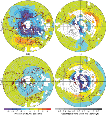
Figure 9.16. Comparison between observed (top) and model-simulated (bottom) December to February sea-level pressure trends (hPa per 50 years) in the NH (left panels) and SH (right panels) based on decadal means for the period 1955 to 2005 . Observed trends are based on the Hadley Centre Mean Sea Level Pressure data set (HadSLP2r, an infilled observational data set; Allan and Ansell, 2006 [JoC, ARC] ). Model-simulated trends are the mean simulated response to greenhouse gas, sulphate aerosol, stratospheric ozone, volcanic aerosol and solar irradiance changes from eight coupled models (CCSM3, GFDL-CM2.0, GFDL-CM2.1, GISS-EH, GISS-ER, MIROC3.2(medres), PCM, UKMO-HadCM3; see Table 8.1 for model descriptions). Streamlines indicate the direction of the trends (ms–1 per 50 years) in the geostrophic wind velocity derived from the trends in sea level pressure, and the shading of the streamlines indicates the magnitude of the change, with darker streamlines corresponding to larger changes in geostrophic wind. White areas in all panels indicate regions with insufficient station-based measurements to constrain analysis. Further explanation of the construction of this figure is provided in the Supplementary Material, Appendix 9.C .Updated after Gillett et al. 2005 [JoC, SRC] ).
The mechanisms underlying NH circulation changes remain open to debate. Simulations in which observed SST changes, which may in part be externally forced, were prescribed either globally or in the tropics alone were able to capture around half of the recent trend towards the positive phase of the NAO ( Hoerling et al., 2005 [JoC] ; Hurrell et al., 2005 [JoC, ARC] ), suggesting that the trend may in part relate to SST changes, particularly over the Indian Ocean ( Hoerling et al., 2005 [JoC] ). Another simulation in which a realistic trend in stratospheric winds was prescribed was able to reproduce the observed trend in the NAO ( Scaife et al., 2005 [PoC, JoC, ARC] Rind et al. 2005a [JoC, SRC] ,b) find that both stratospheric changes and changes in SST can force changes in the NAM and NAO, with changes in SSTs being the dominant forcing mechanism.
Over the period 1968 to 1997, the trend in the NAM was associated with approximately 50% of the winter surface warming in Eurasia, due to increased advection of maritime air onto the continent, but only a small fraction (16%) of the NH extratropical annual mean warming trend ( Thompson et al., 2000 [Ambiguous] ; Section 3.6.4 and Figure 3.30 ). It was also associated with a decrease in winter precipitation over southern Europe and an increase over northern Europe, due the northward displacement of the storm track ( Thompson et al., 2000 [Ambiguous] ).
9.5.3.3 Southern Annular Mode
The SAM is more zonally symmetric than its NH counterpart ( Thompson and Wallace, 2000 [JoC] ; Section 3.6.5 ). It too has exhibited a pronounced upward trend over the past 30 years, corresponding to a decrease in surface pressure over the Antarctic and an increase over the southern mid-latitudes( Figure 9.16 ), although the mean SAM index since 2000 has been below the mean in the late 1990 s, but above the long term mean( Figure 3.32 ). An upward trend in the SAM has occurred in all seasons, but the largest trend has been observed during the southern summer ( Thompson et al., 2000 [Ambiguous] ; Marshall, 2003 [JoC, ARC] Marshall et al. 2004 [JoC, ARC] ) show that observed trends in the SAM are not consistent with simulated internal variability in HadCM3, suggesting an external cause. On the other hand, Jones and Widmann 2004 [JoC, ARC] ) develop a 95-year reconstruction of the summer SAM index based largely on mid-latitude pressure measurements, and find that their reconstructed SAM index was as high in the early 1960 s as in the late 1990 s. However, a more reliable reconstruction from 1958, using more Antarctic data and a different method, indicates that the summer SAM index was higher at the end of the 1990 s than at any other time in the observed record ( Marshall et al., 2004 [JoC, ARC] ).
Based on an analysis of the structure and seasonality of the observed trends in SH circulation, Thompson and Solomon 2002 [PoC, JoC, ARC] ) suggest that they have been largely induced by stratospheric ozone depletion. Several modelling studies simulate an upward trend in the SAM in response to stratospheric ozone depletion ( Sexton, 2001 [JoC, SRC] ; Gillett and Thompson, 2003 [JoC, MoS, SRC] ; Marshall et al., 2004 [JoC, ARC] ; Shindell and Schmidt, 2004 [PoC, JoC, ARC] ; Arblaster and Meehl, 2006 [JoC, MoS, ARC] ; Miller et al., 2006 [PoC, JoC, MoS, ARC] ), particularly in the southern summer. Stratospheric ozone depletion cools and strengthens the antarctic stratospheric vortex in spring, and observations and models indicate that this strengthening of the stratospheric westerlies can be communicated downwards into the troposphere ( Thompson and Solomon, 2002 [PoC, JoC, ARC] ; Gillett and Thompson, 2003 [JoC, MoS, SRC] ). While ozone depletion may be the dominant cause of the trends, other studies have indicated that greenhouse gas increases have also likely contributed ( Fyfe et al., 1999 [JoC, ARC] ; Kushner et al., 2001 [JoC, SRC] ; Stone et al., 2001 [JoC, MoS, SRC] ; Cai et al., 2003 [JoC, SRC] ; Marshall et al., 2004 [JoC, ARC] ; Shindell and Schmidt, 2004 [PoC, JoC, ARC] ; Stone and Fyfe, 2005 [JoC, SRC] ; Arblaster and Meehl, 2006 [JoC, MoS, ARC] ). During the southern summer, the trend in the SAM has been associated with the observed increase of about 3 ms–1 in the circumpolar westerly winds over the Southern Ocean. This circulation change is estimated to explain most of the summer surface cooling over the Antarctic Plateau, and about one-third to one-half of the warming of the Antarctic Peninsula ( Thompson and Solomon, 2002 [PoC, JoC, ARC] ; Carril et al., 2005 [JoC, MoS] ; Section 3.6.5 ), with the largest influence on the eastern side of the Peninsula ( Marshall et al., 2006 [JoC, ARC] ), although other factors are also likely to have contributed to this warming ( Vaughan et al., 2001 [JoC, ARC] ).
9.5.3.4 Sea Level Pressure Detection and Attribution
Global December to February sea level pressure changes observed over the past 50 years have been shown to be inconsistent with simulated internal variability ( Gillett et al., 2003b [JoC, SRC] , 2005 ), but are consistent with the simulated response to greenhouse gas, stratospheric ozone, sulphate aerosol, volcanic aerosol and solar irradiance changes based on 20C3M simulations by eight MMD coupled models ( Gillett et al., 2005 [JoC, SRC] ; Figure 9.16 ). This result is dominated by the SH, where the inclusion of stratospheric ozone depletion leads to consistency between simulated and observed sea level pressure changes. In the NH, simulated sea level pressure trends are much smaller than those observed ( Gillett, 2005 [JoC, SRC] ). Global mean sea level pressure changes associated with increases in atmospheric water vapour are small in comparison to the spatial variations in the observed change in sea level pressure, and are hard to detect because of large observational uncertainties ( Trenberth and Smith, 2005 [PoC, JoC, ARC] ).
The current understanding of climate change in the monsoon regions remains one of considerable uncertainty with respect to circulation and precipitation (Sections 3.7 , 8.4.10 and 10.3.5.2 ). The Asian monsoon circulation in the MMD models was found to decrease by 15% by the late 21st century under the SRES A1B scenario ( Tanaka et al., 2005 [MoS] ; Ueda et al., 2006 [JoC, MoS] ), but trends during the 20th century were not examined. Ramanathan et al. 2005 [JoC, ARC] ) simulate a pronounced weakening of the Asian monsoon circulation between 1985 and 2000 in response to black carbon aerosol increases. ( Chase et al. 2003 ) ) examine changes in several indices of four major tropical monsoonal circulations (Southeastern Asia, western Africa, eastern Africa and the Australia/Maritime Continent) for the period 1950 to 1998 . They find significantly diminished monsoonal circulation in each region, although this result is uncertain due to changes in the observing system affecting the NCEP reanalysis( Section 3.7 ). These results are consistent with simulations ( Ramanathan et al., 2005 [JoC, ARC] ; Tanaka et al., 2005 [MoS] ) of weakening monsoons due to anthropogenic factors, but further model and empirical studies are required to confirm this.
9.5.3.6 Tropical Cyclones
Several recent events, including the active North Atlantic hurricane seasons of 2004 and 2005, the unusual development of a cyclonic system in the subtropical South Atlantic that hit the coast of southern Brazil in March 2004 (e.g., Pezza and Simmonds, 2005 [JoC, ARC] ) and a hurricane close to the Iberian Peninsula in October 2005, have raised public and media interest in the possible effects of climate change on tropical cyclone activity. The TAR concluded that there was ‘no compelling evidence to indicate that the characteristics of tropical and extratropical storms have changed’, but that an increase in tropical peak wind intensities was likely to occur in some areas with an enhanced greenhouse effect (see also Box 3.5 and Trenberth, 2005 [PoC, JoC, ARC] ). The spatial resolution of most climate models limits their ability to realistically simulate tropical cyclones( Section 8.5.3 ), therefore, most studies of projected changes in hurricanes have either used time slice experiments with high-resolution atmosphere models and prescribed SSTs, or embedded hurricane models in lower-resolution General Circulation Models (GCMs)( Section 10.3.6.3 ). While results vary somewhat, these studies generally indicate a reduced frequency of tropical cyclones in response to enhanced greenhouse gas forcing, but an increase in the intensity of the most intense cyclones( Section 10.3.6.3 ). It has been suggested that the simulated frequency reduction may result from a decrease in radiative cooling associated with increased CO2 concentration ( Sugi and Yoshimura, 2004 [JoC, ARC] ; Yoshimura and Sugi, 2005 [ARC] ; Section 10.3.6.3 ; Box 3.5 ), while the enhanced atmospheric water vapour concentration under greenhouse warming increases available potential energy and thus cyclone intensity ( Trenberth, 2005 [PoC, JoC, ARC] ).
There continues to be little evidence of any trend in the observed total frequency of global tropical cyclones, at least up until the late 1990 s (e.g., Solow and Moore, 2002 [JoC] ; Elsner et al., 2004 [JoC, MoS] ; Pielke et al., 2005 [Ambiguous] ; Webster et al., 2005 [JoC] ). However, there is some evidence that tropical cyclone intensity may have increased. Globally, Webster et al. 2005 [JoC] ) find a strong increase in the number and proportion of the most intense tropical cyclones over the past 35 years. Emanuel 2005 [JoC] ) reports a marked increase since the mid- 1970 s in the Power Dissipation Index (PDI), an index of the destructiveness of tropical cyclones (essentially an integral, over the lifetime of the cyclone, of the cube of the maximum wind speed), in the western North Pacific and North Atlantic, reflecting the apparent increases in both the duration of cyclones and their peak intensity. Several studies have shown that tropical cyclone activity was also high in the 1950 to 1970 period in the North Atlantic ( Landsea, 2005 [JoC] ) and North Pacific ( Chan, 2006 [JoC] ), although recent values of the PDI may be higher than those recorded previously ( Emanuel, 2005 [JoC] ; Section 3.8.3 Emanuel 2005 [JoC] and Elsner et al. 2006 [JoC] ) report a strong correlation between the PDI and tropical Atlantic SSTs, although Chan and Liu 2004 [JoC] ) find no analogous relationship in the western North Pacific. While changes in Atlantic SSTs have been linked in part to the AMO, the recent warming appears to be mainly associated with increasing global temperatures( Section 3.8.3.2 ;Mann and Emanuel, 2006 [PoC, JoC] ; Trenberth and Shea, 2006 [PoC, JoC, ARC] ). Tropical cyclone development is also strongly influenced by vertical wind shear and static stability( Box 3.5 ). While increasing greenhouse gas concentrations have likely contributed to a warming of SSTs, effects on static stability and wind shear may have partly opposed this influence on tropical cyclone formation( Box 3.5 ). Thus, detection and attribution of observed changes in hurricane intensity or frequency due to external influences remains difficult because of deficiencies in theoretical understanding of tropical cyclones, their modelling and their long-term monitoring (e.g., Emanuel, 2005 [JoC] ; Landsea, 2005 [JoC] ; Pielke, 2005 [Ambiguous] ). These deficiencies preclude a stronger conclusion than an assessment that anthropogenic factors more likely than not have contributed to an increase in tropical cyclone intensity.
9.5.3.7 Extratropical Cyclones
Simulations of 21st-century climate change in the MMD 20C3M model ensemble generally exhibit a decrease in the total number of extratropical cyclones in both hemispheres, but an increase in the number of the most intense events ( Lambert and Fyfe, 2006 [JoC, MoS, ARC] ), although this behaviour is not reproduced by all models ( Bengtsson et al., 2006 [JoC, ARC] ; Section 10.3.6.4 ). Many 21st-century simulations also show a poleward shift in the storm tracks in both hemispheres ( Bengtsson et al., 2006 [JoC, ARC] ; Section 10.3.6.4 ). Recent observational studies of winter NH storms have found a poleward shift in storm tracks and increased storm intensity, but a decrease in total storm numbers, in the second half of the 20th century( Section 3.5.3 ). Analysis of observed wind and significant wave height suggests an increase in storm activity in the NH. In the SH, the storm track has also shifted poleward, with increases in the radius and depth of storms, but decreases in their frequency. These features appear to be associated with the observed trends in the SAM and NAM. Thus, simulated and observed changes in extratropical cyclones are broadly consistent, but an anthropogenic influence has not yet been detected, owing to large internal variability and problems due to changes in observing systems( Section 3.5.3 ).
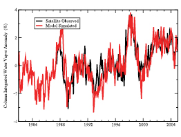
Figure 9.17. Global mean (ocean-only) anomalies relative to 1987 to 2000 in column-integrated water vapour (%) from simulations with the GFDL AM2-LM2 AGCM forced with observed SSTs (red), and satellite observations from SSM/I (black, Wentz and Schabel, 2000 [JoC] ). From Soden et al. 2005 [JoC, ARC] ).
9.5.4 Precipitation
9.5.4.1 Changes in Atmospheric Water Vapour
The amount of moisture in the atmosphere is expected to increase in a warming climate ( Trenberth et al., 2005 [PoC, JoC, ARC] ) because saturation vapour pressure increases with temperature according to the Clausius-Clapeyron equation. Satellite-borne Special Sensor Microwave/Imager (SSM/I) measurements of water vapour since 1988 are of higher quality than either radiosonde or reanalysis data ( Trenberth et al., 2005 [PoC, JoC, ARC] ) and show a statistically significant upward trend in precipitable (column-integrated) water of 1.2 ± 0.3 % per decade averaged over the global oceans( Section 3.4.2.1 Soden et al. 2005 [JoC, ARC] ) demonstrate that the observed changes, including the upward trend, are well simulated in the GFDL atmospheric model when observed SSTs are prescribed( Figure 9.17 ). The simulation and observations show common low-frequency variability, which is largely associated with ENSO. Soden et al. 2005 [JoC, ARC] ) also demonstrate that upper-tropospheric changes in water vapour are realistically simulated by the model. Observed warming over the global oceans is likely largely anthropogenic( Figure 9.12 ), suggesting that anthropogenic influence has contributed to the observed increase in atmospheric water vapour over the oceans.
9.5.4.2 Global Precipitation Changes
The increased atmospheric moisture content associated with warming might be expected to lead to increased global mean precipitation( Section 9.5.4.1 ). Global annual land mean precipitation showed a small, but uncertain, upward trend over the 20th century of approximately 1.1 mm per decade ( Section 3.3.2.1 and Table 3.4 ). However, the record is characterised by large inter-decadal variability, and global annual land mean precipitation shows a non-significant decrease since 1950 ( Figure 9.18 ;see also Table 3.4 ).
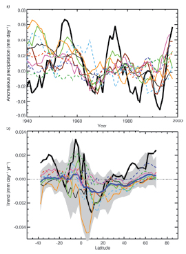
Figure 9.18. Simulated and observed anomalies (with respect to 1961 - 1990 ) in terrestrial mean precipitation (a), and zonal mean precipitation trends 1901 - 1998 (b). Observations (thick black line) are based on a gridded data set of terrestrial rain gauge measurements ( Hulme et al., 1998 [PoC, JoC, MoS, ARC] ). Model data are from 20th-century MMD integrations with anthropogenic, solar and volcanic forcing from the following coupled climate models (see Table 8.1 for model details): UKMO-HadCM3 (brown), CCSM3 (dark blue), GFDL-CM2.0 (pale green), GFDL-CM2.1 (pale blue), GISS-EH (red), GISS-ER (thin black), MIROC3.2(medres) (orange), MRI-CGCM2.3.2 (dark green) and PCM (pink). Coloured curves are ensemble means from individual models. In (a), a five-year running mean was applied to suppress other sources of natural variability, such as ENSO. In (b), the grey band indicates the range of trends simulated by individual ensemble members, and the thick dark blue line indicates the multi-model ensemble mean. External influence in observations on global terrestrial mean precipitation is detected with those precipitation simulations shown by continuous lines in the top panel. Adapted from Lambert et al. 2005 [JoC, MoS, SRC] ).
9.5.4.2.1 Detection of external influence on precipitation
Mitchell et al. 1987 [JoC, MoS] ) argue that global mean precipitation changes should be controlled primarily by the energy budget of the troposphere where the latent heat of condensation is balanced by radiative cooling. Warming the troposphere enhances the cooling rate, thereby increasing precipitation, but this may be partly offset by a decrease in the efficiency of radiative cooling due to an increase in atmospheric CO2 ( Allen and Ingram, 2002 [JoC, MoS, SRC] ; Yang et al., 2003 [JoC] ; Lambert et al., 2004 [JoC, SRC] ; Sugi and Yoshimura, 2004 [JoC, ARC] ). This suggests that global mean precipitation should respond more to changes in shortwave forcing than CO2 forcing, since shortwave forcings, such as volcanic aerosol, alter the temperature of the troposphere without affecting the efficiency of radiative cooling. This is consistent with a simulated decrease in precipitation following large volcanic eruptions ( Robock and Liu, 1994 [JoC, MoS] ; Broccoli et al., 2003 [JoC, MoS, ARC] ), and may explain why anthropogenic influence has not been detected in measurements of global land mean precipitation ( Ziegler et al., 2003 [JoC] ; Gillett et al., 2004b [JoC, SRC] ), although Lambert et al. 2004 [JoC, SRC] ) urge caution in applying the energy budget argument to land-only data. Greenhouse-gas induced increases in global precipitation may have also been offset by decreases due to anthropogenic aerosols ( Ramanathan et al., 2001 [JoC, ARC] ).
Several studies have demonstrated that simulated land mean precipitation in climate model integrations including both natural and anthropogenic forcings is significantly correlated with that observed ( Allen and Ingram, 2002 [JoC, MoS, SRC] ; Gillett et al., 2004b [JoC, SRC] ; Lambert et al., 2004 [JoC, SRC] ), thereby detecting external influence in observations of precipitation (see Section 8.3.1.2 for an evaluation of model-simulated precipitation). Lambert et al. 2005 [JoC, MoS, SRC] ) examine precipitation changes in simulations of nine MMD 20C3M models including anthropogenic and natural forcing( Figure 9.18 a), and find that the responses to combined anthropogenic and natural forcing simulated by five of the nine models are detectable in observed land mean precipitation( Figure 9.18 a). Lambert et al. 2004 [JoC, SRC] ) detect the response to shortwave forcing, but not longwave forcing, in land mean precipitation using HadCM3, and Gillett et al. 2004b [JoC, SRC] ) similarly detect the response to volcanic forcing using the PCM. Climate models appear to underestimate the variance of land mean precipitation compared to that observed ( Gillett et al., 2004b [JoC, SRC] ; Lambert et al., 2004 [JoC, SRC] , 2005 ), but it is unclear whether this discrepancy results from an underestimated response to shortwave forcing ( Gillett et al., 2004b [JoC, SRC] ), underestimated internal variability, errors in the observations, or a combination of these.
Greenhouse gas increases are also expected to cause enhanced horizontal transport of water vapour that is expected to lead to a drying of the subtropics and parts of the tropics ( Kumar et al., 2004 [JoC] ; Neelin et al., 2006 [JoC, MoS] ), and a further increase in precipitation in the equatorial region and at high latitudes ( Emori and Brown, 2005 [JoC, ARC] ; Held and Soden, 2006 [JoC, ARC] ). Simulations of 20th-century zonal mean land precipitation generally show an increase at high latitudes and near the equator, and a decrease in the subtropics of the NH ( Hulme et al., 1998 [PoC, JoC, MoS, ARC] ; Held and Soden, 2006 [JoC, ARC] ; Figure 9.18 b). Projections for the 21st century show a similar effect( Figure 10.12 ). This simulated drying of the northern subtropics and southward shift of the Inter-Tropical Convergence Zone may relate in part to the effects of sulphate aerosol ( Rotstayn and Lohmann, 2002 [JoC, SRC] ), although simulations without aerosol effects also show drying in the northern subtropics ( Hulme et al., 1998 [PoC, JoC, MoS, ARC] ). This pattern of zonal mean precipitation changes is broadly consistent with that observed over the 20th century( Figure 9.18 b; Hulme et al., 1998 [PoC, JoC, MoS, ARC] ; Allen and Ingram, 2002 [JoC, MoS, SRC] ; Rotstayn and Lohmann, 2002 [JoC, SRC] ), although the observed record is characterised by large inter-decadal variability( Figure 3.15 ). The agreement between the simulated and observed zonal mean precipitation trends is not sensitive to the inclusion of forcing by volcanic eruptions in the simulations, suggesting that anthropogenic influence may be evident in this diagnostic.
Changes in runoff have been observed in many parts of the world, with increases or decreases corresponding to changes in precipitation( Section 3.3.4 ). Climate models suggest that runoff will increase in regions where precipitation increases faster than evaporation, such as at high northern latitudes( Section 10.3.2.3 and Figure 10.12 ;see also Milly et al., 2005 [JoC] ; Wu et al., 2005 [JoC, SRC] Gedney et al. 2006 [JoC] ) attribute increased continental runoff in the latter decades of the 20th century in part to suppression of transpiration due to CO2-induced stomatal closure. They find that observed climate changes (including precipitation changes) alone are insufficient to explain the increased runoff, although their result is subject to considerable uncertainty in the runoff data. In addition, Qian et al. 2006 [PoC, JoC, MoS, ARC] ) simulate observed runoff changes in response to observed temperature and precipitation alone, and Milly et al. 2005 [JoC] ) demonstrate that 20th-century runoff trends simulated by the MMD models are significantly correlated with observed runoff trends. Wu et al. 2005 [JoC, SRC] ) demonstrate that observed increases in arctic river discharge are reproduced in coupled model simulations with anthropogenic forcing, but not in simulations with natural forcings only.
Mid-latitude summer drying is another anticipated response to greenhouse gas forcing( Section 10.3.6.1 ), and drying trends have been observed in the both the NH and SH since the 1950 s( Section 3.3.4 Burke et al. 2006 [JoC, MoS] ), using the HadCM3 model with all natural and anthropogenic external forcings and a global Palmer Drought Severity Index data set compiled from observations by Dai et al. 2004 [JoC, ARC] ), are able to formally detect the observed global trend towards increased drought in the second half of the 20th century, although the model trend is weaker than observed and the relative contributions of natural external forcings and anthropogenic forcings are not assessed. The model also simulates some aspects of the spatial pattern of observed drought trends, such as the trends across much of Africa and southern Asia, but not others, such as the trend to wetter conditions in Brazil and northwest Australia.
9.5.4.2.2 Changes in extreme precipitation
Allen and Ingram 2002 [JoC, MoS, SRC] ) suggest that while global annual mean precipitation is constrained by the energy budget of the troposphere, extreme precipitation is constrained by the atmospheric moisture content, as predicted by the Clausius-Clapeyron equation. For a given change in temperature, they therefore predict a larger change in extreme precipitation than in mean precipitation, which is consistent with the HadCM3 response. Consistent with these findings, Emori and Brown 2005 [JoC, ARC] ) discuss physical mechanisms governing changes in the dynamic and thermodynamic components of mean and extreme precipitation and conclude that changes related to the dynamic component (i.e., that due to circulation change) are secondary factors in explaining the greater percentage increase in extreme precipitation than in mean precipitation that is seen in models. Meehl et al. 2005 [JoC, MoS, ARC] ) demonstrate that tropical precipitation intensity increases are related to water vapour increases, while mid-latitude intensity increases are related to circulation changes that affect the distribution of increased water vapour.
Climatological data show that the most intense precipitation occurs in warm regions ( Easterling et al., 2000 [JoC, MoS, ARC] ) and diagnostic analyses have shown that even without any change in total precipitation, higher temperatures lead to a greater proportion of total precipitation in heavy and very heavy precipitation events ( Karl and Trenberth, 2003 [PoC, JoC, ARC] ). In addition, Groisman et al. 1999 [JoC, ARC] ) demonstrate empirically, and Katz 1999 [ARC] ) theoretically, that as total precipitation increases a greater proportion falls in heavy and very heavy events if the frequency remains constant. Similar characteristics are anticipated under global warming ( Cubasch et al., 2001 [NPR, MoS, ARC] ; Semenov and Bengtsson, 2002 [JoC, MoS] ; Trenberth et al., 2003 [PoC, JoC, ARC] Trenberth et al. 2005 [PoC, JoC, ARC] ) point out that since the amount of moisture in the atmosphere is likely to rise much faster as a consequence of rising temperatures than the total precipitation, this should lead to an increase in the intensity of storms, offset by decreases in duration or frequency of events.
Model results also suggest that future changes in precipitation extremes will likely be greater than changes in mean precipitation( Section 10.3.6.1 ;see Section 8.5.2 for an evaluation of model-simulated precipitation extremes). Simulated changes in globally averaged annual mean and extreme precipitation appear to be quite consistent between models. The greater and spatially more uniform increases in heavy precipitation as compared to mean precipitation may allow extreme precipitation change to be more robustly detectable ( Hegerl et al., 2004 [JoC, SRC] ).
Evidence for changes in observations of short-duration precipitation extremes varies with the region considered ( Alexander et al., 2006 [JoC, ARC] ) and the analysis method employed ( Folland et al., 2001 [NPR, PoC, ARC] ; Section 3.8.2.2 ). Significant increases in observed extreme precipitation have been reported over some parts of the world, for example over the USA, where the increase is similar to changes expected under greenhouse warming (e.g., Karl and Knight, 1998 [PoC, JoC, ARC] ; Semenov and Bengtsson, 2002 [JoC, MoS] ; Groisman et al., 2005 [JoC, ARC] ). However, a quantitative comparison between area-based extreme events simulated in models and station data remains difficult because of the different scales involved ( Osborn and Hulme, 1997 [PoC, JoC, MoS, ARC] ). A first attempt based on ( Frich et al. 2002 ) ) indices used fingerprints from atmospheric model simulations with prescribed SST ( Kiktev et al., 2003 [PoC, JoC, MoS, SRC] ) and found little similarity between patterns of simulated and observed rainfall extremes, in contrast to the qualitative similarity found in other studies ( Semenov and Bengtsson, 2002 [JoC, MoS] ; Groisman et al., 2005 [JoC, ARC] Tebaldi et al. 2006 [JoC, MoS, ARC] ) report that eight MMD 20C3M models show a general tendency towards a greater frequency of heavy precipitation events over the past four decades, most coherently at high latitudes of the NH, broadly consistent with observed changes ( Groisman et al., 2005 [JoC, ARC] ).
9.5.4.3 Regional Precipitation Changes
Observed trends in annual precipitation during the period 1901 to 2003 are shown in Figure 3.13 for regions in which data is available. Responses to external forcing in regional precipitation trends are expected to exhibit low signal-to-noise ratios and are likely to exhibit strong spatial variations because of the dependence of precipitation on atmospheric circulation and on geographic factors such as orography. There have been some suggestions, for specific regions, of a possible anthropogenic influence on precipitation, which are discussed below.
9.5.4.3.1 Sahel drought
Rainfall decreased substantially across the Sahel from the 1950 s until at least the late 1980 s ( Dai et al., 2004 [JoC, ARC] ; Figure 9.19 ,see also Figure 3.37 ). There has been a partial recovery since about 1990, although rainfall has not returned to levels typical of the period 1920 to 1965 Zeng 2003 [JoC] ) note that two main hypotheses have been proposed as a cause of the extended drought: overgrazing and conversion of woodland to agriculture increasing surface albedo and reducing moisture supply to the atmosphere, and large-scale atmospheric circulation changes related to decadal global SST changes that could be of anthropogenic or natural origin ( (Nicholson, 2001 ) ). Black carbon has also been suggested as a contributor ( Menon et al., 2002b [JoC, SRC] Taylor et al. 2002 [JoC] ) examine the impact of land use change with an atmospheric GCM forced only by estimates of Sahelian land use change since 1961 . They simulate a small decrease in Sahel rainfall (around 5% by 1996 ) and conclude that the impacts of recent land use changes are not large enough to have been the principal cause of the drought.
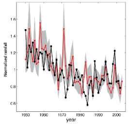
Figure 9.19. Observed (Climatic Research Unit TS 2.1; Mitchell and Jones, 2005 [JoC, ARC] ) Sahel July to September rainfall for each year (black), compared to an ensemble mean of 10 simulations of the atmospheric/land component of the GFDL-CM2.0 model (see Table 8.1 for model details) forced with observed SSTs (red). Both model and observations are normalized to unit mean over 1950 - 2000 . The grey band represents ±1 standard deviation of intra-ensemble variability. After Held et al. 2005 [JoC, MoS, ARC] ), based on results in Lu and Delworth 2005 [JoC, MoS, SRC] ).
Several recent studies have demonstrated that simulations with a range of atmospheric models using prescribed observed SSTs are able to reproduce observed decadal variations in Sahel rainfall ( Bader and Latif, 2003 [JoC, ARC] ; Giannini et al., 2003 [JoC, MoS] ; Rowell, 2003 [JoC] ; Haarsma et al., 2005 [JoC] ; Held et al., 2005 [JoC, MoS, ARC] ; Lu and Delworth, 2005 [JoC, MoS, SRC] ; see also Figure 9.19 ;Hoerling et al., 2006 [JoC, ARC] ), consistent with earlier findings ( Folland, 1986 [PoC, JoC, ARC] ; Rowell, 1996 [JoC] Hoerling et al. 2006 [JoC, ARC] ) show that AGCMs with observed SST changes typically underestimate the magnitude of the observed precipitation changes, although the models and observations are not inconsistent. These studies differ somewhat in terms of which ocean SSTs they find to be most important: Giannini et al. 2003 [JoC, MoS] and Bader and Latif 2003 [JoC, ARC] ) emphasize the role of tropical Indian Ocean warming, Hoerling et al. 2006 [JoC, ARC] ) attribute the drying trend to a progressive warming of the South Atlantic relative to the North Atlantic, and Rowell 2003 [JoC] ) finds that Mediterranean SSTs are an additional important contributor to decadal variations in Sahel rainfall. Based on a multi-model ensemble of coupled model simulations Hoerling et al. 2006 [JoC, ARC] ) conclude that the observed drying trend in the Sahel is not consistent with simulated internal variability alone.
Thus, recent research indicates that changes in SSTs are probably the dominant influence on rainfall in the Sahel, although land use changes possibly also contribute ( Taylor et al., 2002 [JoC] ). But what has caused the differential SST changes? Rotstayn and Lohmann 2002 [JoC, SRC] ) propose that spatially varying, anthropogenic sulphate aerosol forcing (both direct and indirect) can alter low-latitude atmospheric circulation leading to a decline in Sahel rainfall. They find a southward shift of tropical rainfall due to a hemispheric asymmetry in the SST response to changes in cloud albedo and lifetime in a climate simulation forced with recent anthropogenic changes in sulphate aerosol. Williams et al. 2001 [JoC] ) also find a southward shift of tropical rainfall as a response to the indirect effect of sulphate aerosol. These results suggest that sulphate aerosol changes may have led to reduced warming of the northern tropical oceans, which in turn led to the decrease in Sahel rainfall, possibly enhanced through land-atmosphere interaction, although a full attribution analysis has yet to be conducted. Held et al. 2005 [JoC, MoS, ARC] ) show that historical climate simulations with the both the GFDL-CM2.0 and CM2.1 models (see Table 8.1 for details) exhibit drying trends over the Sahel in the second half of the 20th century, which they ascribe to a combination of greenhouse gas and sulphate aerosol changes. The spatial pattern of the trends in simulated rainfall also shows some agreement with observations. However, Hoerling et al. 2006 [JoC, ARC] ) find that eight other coupled climate models with prescribed anthropogenic forcing do not simulate significant trends in Sahel rainfall over the 1950 to 1999 period.
9.5.4.3.2 Southwest Australian drought
Early winter (May–July) rainfall in the far southwest of Australia declined by about 15% in the mid- 1970 s ( IOCI, 2002 [NPR] ) and remained low subsequently. The rainfall decrease was accompanied by a change in large-scale atmospheric circulation in the surrounding region ( Timbal, 2004 [MoS] ). The circulation and precipitation changes are somewhat consistent with, but larger than, those simulated by climate models in response to greenhouse gas increases. The Indian Ocean Climate Initiative ( IOCI, 2005 [NPR] ) concludes that land cover change could not be the primary cause of the rainfall decrease because of the link between the rainfall decline and changes in large-scale atmospheric circulation, and re-affirms the conclusion of IOCI 2002 [NPR] ) that both natural variability and greenhouse forcing likely contributed. Timbal et al. 2005 [JoC, SRC] ) demonstrate that climate change signals downscaled from the PCM show some similarity to observed trends, although the significance of this finding is uncertain.
Some authors (e.g., Karoly, 2003 [Ambiguous] ) have suggested that the decrease in rainfall is related to anthropogenic changes in the SAM (see Section 9.5.3.3 ). However, the influence of changes in circulation on southwest Australian drought remains unclear as the largest SAM trend has occurred during the SH summer (December–March; Thompson et al., 2000 [Ambiguous] ; Marshall et al., 2004 [JoC, ARC] ), while the largest rainfall decrease has occurred in early winter (May–July).
9.5.4.3.3 Monsoon precipitation
Decreasing trends in precipitation over the Indonesian Maritime Continent, equatorial western and central Africa, Central America, Southeast Asia and eastern Australia have been observed over the period 1948 to 2003, while increasing trends were found over the USA and north-western Australia( Section 3.7 ). The TAR ( IPCC, 2001 [NPR] , pp. 568) concluded that an increase in Southeast Asian summer monsoon precipitation is simulated in response to greenhouse gas increases in climate models, but that this effect is reduced by an increase in sulphate aerosols, which tend to decrease monsoon precipitation. Since then, additional modelling studies have come to conflicting conclusions regarding changes in monsoon precipitation ( (Lal and Singh, 2001; ) Douville et al., 2002 [JoC] ; Maynard et al., 2002 [JoC] ; May, 2004; Wardle and Smith, 2004 [JoC, MoS] ; see also Section 9.5.3.5 Ramanathan et al. 2005 [JoC, ARC] ) were able to simulate realistic changes in Indian monsoon rainfall, particularly a decrease that occurred between 1950 and 1970, by including the effects of black carbon aerosol. In both the observations and model, these changes were associated with a decreased SST gradient over the Indian Ocean and an increase in tropospheric stability, and they were not reproduced in simulations with greenhouse gas and sulphate aerosol changes only.
9.5.5 Cryosphere Changes
9.5.5.1 Sea Ice
Widespread warming would, in the absence of other countervailing effects, lead to declines in sea ice, snow, and glacier and ice sheet extent and thickness. The annual mean area of arctic sea ice cover has decreased in recent decades, with stronger declines in summer than in winter, and some thinning( Section 4.4 Gregory et al. 2002b [JoC, MoS, SRC] ) show that a four-member ensemble of HadCM3 integrations with all major anthropogenic and natural forcing factors simulates a decline in arctic sea ice extent of about 2.5% per decade over the period 1970 to 1999, which is close to the observed decline of 2.7% per decade over the satellite period 1978 to 2004 . This decline is inconsistent with simulated internal climate variability and the response to natural forcings alone ( Vinnikov et al., 1999 [JoC] ; Gregory et al., 2002b [JoC, MoS, SRC] ; Johannssen et al., 2004 [JoC, MoS] ), indicating that anthropogenic forcing has likely contributed to the trend in NH sea ice extent. Models such as those described by Rothrock et al. 2003 [JoC, MoS, ARC] ) and references therein are able to reproduce the observed interannual variations in ice thickness, at least when averaged over fairly large regions. Simulations of historical arctic ice thickness or volume ( Goeberle and Gerdes, 2003 [JoC, ARC] ; Rothrock et al., 2003 [JoC, MoS, ARC] ) show a marked reduction in ice thickness starting in the late 1980 s, but disagree somewhat with respect to trends and/or variations earlier in the century. Although some of the dramatic change inferred may be a consequence of a spatial redistribution of ice volume over time (e.g., Holloway and Sou, 2002 [JoC] ), thermodynamic changes are also believed to be important. Low-frequency atmospheric variability (such as interannual changes in circulation connected to the NAM) appears to be important in flushing ice out of the Arctic Basin, thus increasing the amount of summer open water and enhancing thermodynamic thinning through the ice-albedo feedback (e.g., Lindsay and Zhang, 2005 [JoC] ). Large-scale modes of variability affect both wind driving and heat transport in the atmosphere, and therefore contribute to interannual variations in ice formation, growth and melt (e.g., Rigor et al., 2002 [JoC, ARC] ; Dumas et al., 2003 [JoC, MoS, ARC] ). Thus, the decline in arctic sea ice extent and its thinning appears to be largely, but not wholly, due to greenhouse gas forcing.
Unlike in the Arctic, a strong decline in sea ice extent has not been observed in the Antarctic during the period of satellite observations( Section 4.4.2.2 Fichefet et al. 2003 [JoC, MoS, SRC] ) conducted a simulation of Antarctic ice thickness using observationally based atmospheric forcing covering the period 1958 to 1999 . They note pronounced decadal variability, with area average ice thickness varying by ±0.1 m (compared to a mean thickness of roughly 0.9 m), but no long-term trend. However, Gregory et al. 2002b [JoC, MoS, SRC] ) find a decline in antarctic sea ice extent in their model, contrary to observations. They suggest that the lack of consistency between the observed and modelled changes in sea ice extent might reflect an unrealistic simulation of regional warming around Antarctica, rather than a deficiency in the ice model. Holland and Raphael 2006 [JoC, MoS, ARC] ) examine sea ice variability in six MMD 20C3M simulations that include stratospheric ozone depletion. They conclude that the observed weak increase in antarctic sea ice extent is not inconsistent with simulated internal variability, with some simulations reproducing the observed trend over 1979 to 2000, although the models exhibit larger interannual variability in sea ice extent than satellite observations.
9.5.5.2 Snow and Frozen Ground
Snow cover in the NH, as measured from satellites, has declined substantially in the past 30 years, particularly from early spring through summer( Section 4.2 ). Trends in snow depth and cover can be driven by precipitation or temperature trends. The trends in recent decades have generally been driven by warming at lower and middle elevations. Evidence for this includes: (a) interannual variations in NH April snow-covered area are strongly correlated (r = –0.68) with April 40°N to 60°N temperature; (b) interannual variations in snow (water equivalent, depth or duration) are strongly correlated with temperature at lower- and middle-elevation sites in North America ( Mote et al., 2005 [JoC, ARC] ), Switzerland ( Scherrer et al., 2004 [JoC, ARC] ) and Australia ( Nicholls, 2005 [SRC] ); (c) trends in snow water equivalent or snow depth show strong dependence on elevation or equivalently mean winter temperature, both in western North America and Switzerland (with stronger decreases at lower, warmer elevations where a warming is more likely to affect snowfall and snowmelt); and (d) the trends in North America, Switzerland and Australia have been shown to be well explained by warming and cannot be explained by changes in precipitation. In some very cold places, increases in snow depth have been observed and have been linked to higher precipitation.
Widespread permafrost warming and degradation appear to be the result of increased summer air temperatures and changes in the depth and duration of snow cover( Section 4.7.2 ). The thickness of seasonally frozen ground has decreased in response to winter warming and increases in snow depth( Section 4.7.3 ).
9.5.5.3 Glaciers, Ice Sheets and Ice Shelves
During the 20th century, glaciers generally lost mass with the strongest retreats in the 1930 s and 1940 s and after 1990 ( Section 4.5 ). The widespread shrinkage appears to imply widespread warming as the probable cause ( Oerlemans, 2005 [JoC, ARC] ), although in the tropics changes in atmospheric moisture might be contributing( Section 4.5.3 ). Over the last half century, both global mean winter accumulation and summer melting have increased steadily ( Ohmura, 2004 [NPR, ARC] ; Dyurgerov and Meier, 2005 [NPR, ARC] ;( Greene, 2005 ) ), and at least in the NH, winter accumulation and summer melting correlate positively with hemispheric air temperature ( (Greene, 2005 ) ); the negative correlation of net balance with temperature indicates the primary role of temperature in forcing the respective glacier fluctuations.
There have been a few studies for glaciers in specific regions examining likely causes of trends. Mass balances for glaciers in western North America are strongly correlated with global mean winter (October–April) temperatures and the decline in glacier mass balance has paralleled the increase in temperature since 1968 ( Meier et al., 2003 [JoC, ARC] Reichert et al. 2002a [JoC, ARC] ) forced a glacier mass balance model for the Nigardsbreen and Rhône glaciers with downscaled data from an AOGCM control simulation and conclude that the rate of glacier advance during the ‘Little Ice Age’ could be explained by internal climate variability for both glaciers, but that the recent retreat cannot, implying that the recent retreat of both glaciers is probably due to externally forced climate change. As well, the thinning and acceleration of some polar glaciers (e.g., Thomas et al., 2004 [JoC, ARC] ) appear to be the result of ice sheet calving driven by oceanic and atmospheric warming( Section 4.6.3.4 ).
Taken together, the ice sheets of Greenland and Antarctica are shrinking. Slight thickening in inland Greenland is more than compensated for by thinning near the coast( Section 4.6.2.2 ). Warming is expected to increase low-altitude melting and high-altitude precipitation in Greenland; altimetry data suggest that the former effect is dominant. However, because some portions of ice sheets respond only slowly to climate changes, past forcing may be influencing ongoing changes, complicating attribution of recent trends( Section 4.6.3.2 ).
9.5.6 Summary
In the TAR, quantitative evidence for human influence on climate was based almost exclusively on atmospheric and surface temperature. Since then, anthropogenic influence has also been identified in a range of other climate variables, such as ocean heat content, atmospheric pressure and sea ice extent, thereby contributing further evidence of an anthropogenic influence on climate, and improving confidence in climate models.
Observed changes in ocean heat content have now been shown to be inconsistent with simulated natural climate variability, but consistent with a combination of natural and anthropogenic influences both on a global scale, and in individual ocean basins. Models suggest a substantial anthropogenic contribution to sea level rise, but underestimate the actual rise observed. While some studies suggest that an anthropogenic increase in high-latitude rainfall may have contributed to a freshening of the Arctic Ocean and North Atlantic deep water, these results are still uncertain.
There is no evidence that 20th-century ENSO behaviour is distinguishable from natural variability. By contrast, there has been a detectable human influence on global sea level pressure. Both the NAM and SAM have shown significant trends. Models reproduce the sign but not magnitude of the NAM trend, and models including both greenhouse gas and ozone simulate a realistic trend in the SAM. Anthropogenic influence on either tropical or extratropical cyclones has not been detected, although the apparent increased frequency of intense tropical cyclones, and its relationship to ocean warming, is suggestive of an anthropogenic influence.
Simulations and observations of total atmospheric water vapour averaged over oceans agree closely when the simulations are constrained by observed SSTs, suggesting that anthropogenic influence has contributed to an increase in total atmospheric water vapour. However, global mean precipitation is controlled not by the availability of water vapour, but by a balance between the latent heat of condensation and radiative cooling in the troposphere. This may explain why human influence has not been detected in global precipitation, while the influence of volcanic aerosols has been detected. However, observed changes in the latitudinal distribution of land precipitation are suggestive of a possible human influence as is the observed increased incidence of drought as measured by the Palmer Drought Severity Index. Observational evidence indicates that the frequency of the heaviest rainfall events has likely increased within many land regions in general agreement with model simulations that indicate that rainfall in the heaviest events is likely to increase in line with atmospheric water vapour concentration. Many AGCMs capture the observed decrease in Sahel rainfall when constrained by observed SSTs, although this decrease is not simulated by most AOGCMs. One study found that an observed decrease in Asian monsoon rainfall could only be simulated in response to black carbon aerosol, although conclusions regarding the monsoon response to anthropogenic forcing differ.
Observed decreases in arctic sea ice extent have been shown to be inconsistent with simulated internal variability, and consistent with the simulated response to human influence, but SH sea ice extent has not declined. The decreasing trend in global snow cover and widespread melting of glaciers is consistent with a widespread warming. Anthropogenic forcing has likely contributed substantially to widespread glacier retreat during the 20th century.
9.6 Observational Constraints on Climate Sensitivity
This section assesses recent research that infers equilibrium climate sensitivity and transient climate response from observed changes in climate. ‘Equilibrium climate sensitivity’ (ECS) is the equilibrium annual global mean temperature response to a doubling of equivalent atmospheric CO2 from pre-industrial levels and is thus a measure of the strength of the climate system’s eventual response to greenhouse gas forcing. ‘Transient climate response’ (TCR) is the annual global mean temperature change at the time of CO2 doubling in a climate simulation with a 1% yr–1 compounded increase in CO2 concentration (see Glossary and Section 8.6.2.1 for detailed definitions). TCR is a measure of the strength and rapidity of the climate response to greenhouse gas forcing, and depends in part on the rate at which the ocean takes up heat. While the direct temperature change that results from greenhouse gas forcing can be calculated in a relatively straightforward manner, uncertain atmospheric feedbacks( Section 8.6 )lead to uncertainties in estimates of future climate change. The objective here is to assess estimates of ECS and TCR that are based on observed climate changes, while Chapter8 assesses feedbacks individually. Inferences about climate sensitivity from observed climate changes complement approaches in which uncertain parameters in climate models are varied and assessed by evaluating the resulting skill in reproducing observed mean climate( Section 10.5.4.4 ). While observed climate changes have the advantage of being most clearly related to future climate change, the constraints they provide on climate sensitivity are not yet very strong, in part because of uncertainties in both climate forcing and the estimated response( Section 9.2 ). An overall summary assessment of ECS and TCR, based on the ability of models to simulate climate change and mean climate and on other approaches, is given in Box 10.2 .Note also that this section does not assess regional climate sensitivity or sensitivity to forcings other than CO2.
9.6.1 Methods to Estimate Climate Sensitivity
The most straightforward approach to estimating climate sensitivity would be to relate an observed climate change to a known change in radiative forcing. Such an approach is strictly correct only for changes between equilibrium climate states. Climatic states that were reasonably close to equilibrium in the past are often associated with substantially different climates than the pre-industrial or present climate, which is probably not in equilibrium ( Hansen et al., 2005 [JoC, ARC] ). An example is the climate of the LGM( Chapter6 and Section 9.3 ). However, the climate’s sensitivity to external forcing will depend on the mean climate state and the nature of the forcing, both of which affect feedback mechanisms( Chapter8 ). Thus, an estimate of the sensitivity directly derived from the ratio of response to forcing cannot be readily compared to the sensitivity of climate to a doubling of CO2 under idealised conditions. An alternative approach, which has been pursued in most work reported here, is based on varying parameters in climate models that influence the ECS in those models, and then attaching probabilities to the different ECS values based on the realism of the corresponding climate change simulations. This ameliorates the problem of feedbacks being dependent on the climatic state, but depends on the assumption that feedbacks are realistically represented in models and that uncertainties in all parameters relevant for feedbacks are varied. Despite uncertainties, results from simulations of climates of the past and recent climate change (Sections 9.3 to 9.5 )increase confidence in this assumption.
The ECS and TCR estimates discussed here are generally based on large ensembles of simulations using climate models of varying complexity, where uncertain parameters influencing the model’s sensitivity to forcing are varied. Studies vary key climate and forcing parameters in those models, such as the ECS, the rate of ocean heat uptake, and in some instances, the strength of aerosol forcing, within plausible ranges. The ECS can be varied directly in simple climate models and in some EMICs (see Chapter8 ), and indirectly in more complex EMICs and AOGCMs by varying model parameters that influence the strength of atmospheric feedbacks, for example, in cloud parametrizations. Since studies estimating ECS and TCR from observed climate changes require very large ensembles of simulations of past climate change (ranging from several hundreds to thousands of members), they are often, but not always, performed with EMICs or EBMs.
The idea underlying this approach is that the plausibility of a given combination of parameter settings can be determined from the agreement of the resulting simulation of historical climate with observations. This is typically evaluated by means of Bayesian methods (see Supplementary Material, Appendix 9.B for methods). Bayesian approaches constrain parameter values by combining prior distributions that account for uncertainty in the knowledge of parameter values with information about the parameters estimated from data ( Kennedy and O’Hagan, 2001 [MoS] ). The uniform distribution has been used widely as a prior distribution, which enables comparison of constraints obtained from the data in different approaches. ECS ranges encompassed by the uniform prior distribution must be limited due to computer time limiting the size of model ensembles, but generally cover the range considered possible by experts, such as from 0°C to 10°C. Note that uniform prior distributions for ECS, which only require an expert assessment of possible range, generally assign a higher prior belief to high sensitivity than, for example, non-uniform prior distributions that depend more heavily on expert assessments (e.g., Forest et al., 2006 [JoC, MoS, ARC] ). In addition, Frame et al. 2005 [JoC, MoS] ) point out that care must be taken when specifying the uniform prior distribution. For example, a uniform prior distribution for the climate feedback parameter (see Glossary) implies a non-uniform prior distribution for ECS due to the nonlinear relationship between the two parameters.
Since observational constraints on the upper bound of ECS are still weak (as shown below), these prior assumptions influence the resulting estimates. Frame et al. 2005 [JoC, MoS] ) advocate sampling a flat prior distribution in ECS if this is the target of the estimate, or in TCR if future temperature trends are to be constrained. In contrast, statistical research on the design and interpretation of computer experiments suggests the use of prior distributions for model input parameters (e.g., see Kennedy and O’Hagan, 2001 [MoS] ; Goldstein and Rougier, 2004 [MoS] ). In such Bayesian studies, it is generally good practice to explore the sensitivity of results to different prior beliefs (see, for example, Tol and Vos, 1998 [NotFound] ; O’Hagan and Forster, 2004 [NPR] ). Furthermore, as demonstrated by Annan and Hargreaves 2005 [NotFound] and Hegerl et al. 2006a [NPR, PoC, JoC, SRC] ), multiple and independent lines of evidence about climate sensitivity from, for example, analysis of climate change at different times, can be combined by using information from one line of evidence as prior information for the analysis of another line of evidence. The extent to which the different lines of evidence provide complete information on the underlying physical mechanisms and feedbacks that determine the climate sensitivity is still an area of active research. In the following, uniform prior distributions for the target of the estimate are used unless otherwise specified.
Methods that incorporate a more comprehensive treatment of uncertainty generally produce wider uncertainty ranges for the inferred climate parameters. Methods that do not vary uncertain parameters, such as ocean diffusivity, in the course of the uncertainty analysis will yield probability distributions for climate sensitivity that are conditional on these values, and therefore are likely to underestimate the uncertainty in climate sensitivity. On the other hand, approaches that do not use all available evidence will produce wider uncertainty ranges than estimates that are able to use observations more comprehensively.
9.6.2 Estimates of Climate Sensitivity Based on Instrumental Observations
9.6.2.1 Estimates of Climate Sensitivity Based on 20th-Century Warming
Anumber of recent studies have used instrumental records of surface, ocean and atmospheric temperature changes to estimate climate sensitivity. Most studies use the observed surface temperature changes over the 20th century or the last 150 years( Chapter3 ). In addition, some studies also use the estimated ocean heat uptake since 1955 based on Levitus et al. 2000 [JoC, ARC] , 2005 )( Chapter5 ), and temperature changes in the free atmosphere( Chapter3 ;see also Table 9.3 ). For example, Frame et al. 2005 [JoC, MoS] and Andronova and Schlesinger 2000 [JoC, SRC] ) use surface air temperature alone, while Forest et al. 2002 [JoC, SRC] , 2006 Knutti et al. 2002 [PoC, JoC, MoS, SRC] , 2003 and Gregory et al. 2002a [JoC, MoS, SRC] ) use both surface air temperature and ocean temperature change to constrain climate sensitivity. Forest et al. 2002 [JoC, SRC] , 2006 and Lindzen and Giannitsis 2002 [NPR, JoC] ) use free atmospheric temperature data from radiosondes in addition to surface air temperature. Note that studies using radiosonde data may be affected by recently discovered inhomogeneities( Section 3.4.1.1 ), although Forest et al. 2006 [JoC, MoS, ARC] ) illustrate that the impact of the radiosonde atmospheric temperature data on their climate sensitivity estimate is smaller than that of surface and ocean warming data. A further recent study uses Earth Radiation Budget Experiment (ERBE) data ( Forster and Gregory, 2006 [JoC, SRC] ) in addition to surface temperature changes to estimate climate feedbacks (and thus ECS) from observed changes in forcing and climate.
Wigley et al. 1997 [PoC, JoC, ARC] ) pointed out that uncertainties in forcing and response made it impossible to use observed global temperature changes to constrain ECS more tightly than the range explored by climate models at the time (1.5°C to 4.5°C), and particularly the upper end of the range, a conclusion confirmed by subsequent studies. A number of subsequent publications qualitatively describe parameter values that allow models to reproduce features of observed changes, but without directly estimating a climate sensitivity probability density function (PDF). For example, Harvey and Kaufmann 2002 [JoC, MoS] ) find a best-fit ECS of 2.0°C out of a range of 1°C to 5°C, and constrain fossil fuel and biomass aerosol forcing( Section 9.2.1.2 Lindzen and Giannitsis 2002 [NPR, JoC] ) pose the hypothesis that the rapid change in tropospheric (850–300 hPa) temperatures around 1976 triggered a delayed response in surface temperature that is best modelled with a climate sensitivity of less than 1°C. However, their estimate does not account for substantial uncertainties in the analysis of such a short time period, most notably those associated with the role of internal climate variability in the rapid tropospheric warming of 1976 . The 1976 – 1977 climate shift occurred along with a phase shift of the PDO, and a concurrent change in the ocean( Section 3.6.3 )that appears to contradict the Lindzen and Giannitsis 2002 [NPR, JoC] ) assumption that the change was initiated by tropospheric forcing. In addition, the authors do not account for uncertainties in the simple model whose sensitivity is fitted. The finding of Lindzen and Giannitsis is in contrast with that of Forest et al. 2002 [JoC, SRC] , 2006 ) who consider the joint evolution of surface and upper air temperatures on much longer time scales.
Several recent studies have derived probability estimates for ECS using a range of models and diagnostics. The diagnostics, which are used to compare model-simulated and observed changes, are often simple temperature indices such as the global mean surface temperature and ocean mean warming ( Knutti et al., 2002 [PoC, JoC, MoS, SRC] , 2003 ) or the differential warming between the SH and NH (together with the global mean; Andronova and Schlesinger, 2001 [JoC, MoS, SRC] ). Results that use more detailed information about the space-time evolution of climate may be able to provide tighter constraints than those that use simpler indices. Forest et al. 2002 [JoC, SRC] , 2006 ) use a so-called ‘optimal’ detection method( Section 9.4.1.4 and Appendix 9.A.1) to diagnose the fit between model-simulated and observed patterns of zonal mean temperature change. Frame et al. 2005 [JoC, MoS] ) use detection results from an analysis based on several multi-model AOGCM fingerprints( Section 9.4.1.4 )that separate the greenhouse gas response from that to other anthropogenic and natural forcings ( Stott et al., 2006c [JoC, MoS, SRC] ). Similarly, Gregory et al. 2002a [JoC, MoS, SRC] ) apply an inverse estimate of the range of aerosol forcing based on fingerprint detection results. Note that while results from fingerprint detection approaches will be affected by uncertainty in separation between greenhouse gas and aerosol forcing, the resulting uncertainty in estimates of the near-surface temperature response to greenhouse gas forcing is relatively small (Sections 9.2.3 and 9.4.1.4 ).
Afurther consideration in assessing these results is the extent to which realistic forcing estimates were used, and whether forcing uncertainty was included. Most studies consider a range of anthropogenic forcing factors, including greenhouse gases and sulphate aerosol forcing, sometimes directly including the indirect forcing effect, such as Knutti et al. 2002 [PoC, JoC, MoS, SRC] , 2003 ), and sometimes indirectly accounting for the indirect effect by using a wide range of direct forcing (e.g., Andronova and Schlesinger, 2001 [JoC, MoS, SRC] ; Forest et al., 2002 [JoC, SRC] , 2006 ). Many studies also consider tropospheric ozone (e.g., Andronova and Schlesinger, 2001 [JoC, MoS, SRC] ; Knutti et al., 2002 [PoC, JoC, MoS, SRC] , 2003 Forest et al. 2006 [JoC, MoS, ARC] ) demonstrate that the inclusion of natural forcing affects the estimated PDF of climate sensitivity since net negative natural forcing in the second half of the 20th century favours higher sensitivities than earlier results that disregarded natural forcing ( Forest et al., 2002 [JoC, SRC] ; see Figure 9.20 ), particularly if the same ocean warming estimates were used. Note that some of the changes due to inclusion of natural forcing are offset by using recently revised ocean warming data ( Levitus et al., 2005 [JoC, ARC] ), which favour somewhat smaller ocean heat uptakes than earlier data ( Levitus et al., 2001 [JoC, ARC] ; Forest et al., 2006 [JoC, MoS, ARC] ). Only a few estimates account for uncertainty in forcings other than from aerosols (e.g., Gregory et al., 2002a [JoC, MoS, SRC] ; Knutti et al., 2002 [PoC, JoC, MoS, SRC] , 2003 ); some other studies perform some sensitivity testing to assess the effect of forcing uncertainty not accounted for, for example, in natural forcing (e.g., Forest et al., 2006 [JoC, MoS, ARC] ; see Table 9.1 for an overview).
The treatment of uncertainty in the ocean’s uptake of heat varies, from assuming a fixed value for a model’s ocean diffusivity ( Andronova and Schlesinger, 2001 [JoC, MoS, SRC] ) to trying to allow for a wide range of ocean mixing parameters ( Knutti et al., 2002 [PoC, JoC, MoS, SRC] , 2003 ) or systematically varying the ocean’s effective diffusivity (e.g., Forest et al., 2002 [JoC, SRC] , 2006; Frame et al., 2005 [JoC, MoS] ). Furthermore, all approaches that use the climate’s time evolution attempt to account for uncertainty due to internal climate variability, either by bootstrapping ( Andronova and Schlesinger, 2001 [JoC, MoS, SRC] ), by using a noise model in fingerprint studies whose results are used ( Frame et al., 2005 [JoC, MoS] ) or directly ( Forest et al., 2002 [JoC, SRC] , 2006 ).
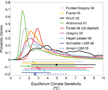
Figure 9.20. Comparison between different estimates of the PDF (or relative likelihood) for ECS (°C). All PDFs/likelihoods have been scaled to integrate to unity between 0°C and 10°C ECS. The bars show the respective 5 to 95% ranges, dots the median estimate. The PDFs/likelihoods based on instrumental data are from Andronova and Schlesinger 2001 [JoC, MoS, SRC] Forest et al. 2002 [JoC, SRC] ; dashed line, considering anthropogenic forcings only), Forest et al. 2006 [JoC, MoS, ARC] ; solid, anthropogenic and natural forcings), Gregory et al. 2002a [JoC, MoS, SRC] Knutti et al. 2002 [PoC, JoC, MoS, SRC] Frame et al. 2005 [JoC, MoS] and Forster and Gregory 2006 [JoC, SRC] ), transformed to a uniform prior distribution in ECS using the method after Frame et al. 2005 [JoC, MoS] Hegerl et al. 2006a [NPR, PoC, JoC, SRC] ) is based on multiple palaeoclimatic reconstructions of NH mean temperatures over the last 700 years. Also shown are the 5 to 95% approximate ranges for two estimates from the LGM (dashed, Annan et al., 2005 [MoS, ARC] ; solid, Schneider von Deimling et al., 2006 [PoC, JoC, MoS, ARC] ) which are based on models with different structural properties. Note that ranges extending beyond the published range in Annan et al. 2005 [MoS, ARC] ), and beyond that sampled by the climate model used there, are indicated by dots and an arrow, since Annan et al. only provide an upper limit. For details of the likelihood estimates, see Table 9.3 .After Hegerl et al. 2006a [NPR, PoC, JoC, SRC] ).
Figure 9.20 compares results from many of these studies. All PDFs shown are based on a uniform prior distribution of ECS and have been rescaled to integrate to unity for all positive sensitivities up to 10°C to enable comparisons of results using different ranges of uniform prior distributions (this affects both median and upper 95th percentiles if original estimates were based on a wider uniform range). Thus, zero prior probability is assumed for sensitivities exceeding 10°C, since many results do not consider those, and for negative sensitivities. Negative climate sensitivity would lead to cooling in response to a positive forcing and is inconsistent with understanding of the energy balance of the system ( Stouffer et al., 2000 [JoC, MoS, SRC] ; Gregory et al., 2002a [JoC, MoS, SRC] ; Lindzen and Giannitsis, 2002 [NPR, JoC] ). This figure shows that best estimates of the ECS (mode of the estimated PDFs) typically range between 1.2°C and 4°C when inferred from constraints provided by historical instrumental data, in agreement with estimates derived from more comprehensive climate models. Most studies suggest a 5th percentile for climate sensitivity of 1°C or above. The upper 95th percentile is not well constrained, particularly in studies that account conservatively for uncertainty in, for example, 20th-century radiative forcing and ocean heat uptake. The upper tail is particularly long in studies using diagnostics based on large-scale mean data because separation of the greenhouse gas response from that to aerosols or climate variability is more difficult with such diagnostics ( Andronova and Schlesinger, 2001 [JoC, MoS, SRC] ; Gregory et al., 2002a [JoC, MoS, SRC] ; Knutti et al., 2002 [PoC, JoC, MoS, SRC] , 2003 Forest et al. 2006 [JoC, MoS, ARC] ) find a 5 to 95% range of 2.1°C to 8.9°C for climate sensitivity( Table 9.3 ), which is a wider range than their earlier result based on anthropogenic forcing only ( Forest et al., 2002 [JoC, SRC] Frame et al. 2005 [JoC, MoS] ) infer a 5 to 95% uncertainty range for the ECS of 1.2°C to 11.8°C, using a uniform prior distribution that extends well beyond 10°C sensitivity. Studies generally do not find meaningful constraints on the rate at which the climate system mixes heat into the deep ocean (e.g., Forest et al., 2002 [JoC, SRC] , 2006 ). However, Forest et al. 2006 [JoC, MoS, ARC] ) find that many coupled AOGCMs mix heat too rapidly into the deep ocean, which is broadly consistent with comparisons based on heat uptake( Section 9.5.1.1 ,). However the relevance of this finding is unclear because most MMD AOGCMs were not included in the Forest et al. comparison, and because they used a relatively simple ocean model. Knutti et al. 2002 [PoC, JoC, MoS, SRC] ) also determine that strongly negative aerosol forcing, as has been suggested by several observational studies ( Anderson et al., 2003 [JoC, MoS] ), is incompatible with the observed warming trend over the last century( Section 9.2.1.2 and Table 9.1 ).
Table 9.3. Results from key studies on observational estimates of ECS (in °C) from instrumental data, individual volcanic eruptions, data for the last millennium, and simulations of the LGM . The final three rows list some studies using non-uniform prior distributions, while the other studies use uniform prior distributions of ECS.
| Study | Observational Data Used to Constrain Studya | Modelb | External Forcings Includedc | Treatment of uncertaintiesd | Estimated ECS Range 5to 95% (°C) |
|---|---|---|---|---|---|
| From Instrumental Data | |||||
| Forest et al. (2006) | Upper air, surface and deep ocean space-time 20th-century temperatures Prior 0°C to 10°C | 2-D EMIC (~E6) | G, Sul, Sol, Vol, OzS, land surface changes (2002: G, Sul, OzS) | εobs,noise, k, εaer,sensitivity tests for solar/volcanic. forcing uncertainty | 2.1 to 8.9 (1.4 to 7.7 without natural forcings) |
| Andronova and Schlesinger (2001) | Global mean and hemispheric difference in surface air temperature 1856 to 1997 | EBM | G, OzT, Sul, Sol, Vol | Noise (bootstrap residual), choice of radiative forcing factors | 1.0 to 9.3 prob ~ 54% that ECS outside 1.5 to 4.5 |
| Knutti et al. (2002; 2003) | Global mean ocean heat uptake 1955 to 1995, mean surface air temperature 1860 to 2000 Prior 0°C to 10°C | EMIC (~E1) plus neural net | G, OzT, OzS, fossil fuel and biomass burning BC+OM, stratospheric water vapour, Vol, Sol, Sul, Suli | εobs,εforc for multiple forcings from IPCC (2001), k, different ocean mixing schemes | 2.2 to 9.2 prob ~ 50% that ECS outside 1.5 to 4.5 |
| Gregory et al. (2002a) | Global mean change in surface air temperature and ocean heat change between 1861 to 1900 and 1957 to 1994 | 1-Box | G, Sul and Suli (top down via Stott et al., 2001), Sol, Vol | εobs,εforc | 1.1 to ∞ |
| Frame et al. (2005) | Global change in surface temperature | EBM | G, accounted for other anthropogenic and natural forcing by fingerprints, Sul, Nat | Noise, uncertainty in amplitude but not pattern of natural and anthropogenic. forcings and response (scaling factors), k (range consistent with ocean warming) | 1.2 to 11.8 |
| Study | Observational Data Used to Constrain Studya | Modelb | External Forcings Includedc | Treatment of uncertaintiesd | Estimated ECS Range 5to 95% (°C) |
| Forster and Gregory (2006) | 1985 to 1996 ERBE data 60°N to 60°S, global surface temperature Prior 0°C to 18.5°C, transformed after Frame et al. (2005) | 1-Box | G, Vol, Sol, Sul | εobs,εforc | 1.2 to 14.2 |
| From individual volcanic eruptions | |||||
| Wigley et al. (2005a) | Global mean surface temperature | EBM | From volcanic forcing only | El Niño | Agung: 1.3 to 6.3; El Chichon: 0.3 to 7.7; Mt. Pinatubo: 1.8 to 5.2 |
| From last millenium | |||||
| Hegerl et al. (2006a) | NH mean surface air temperature pre-industrial (1270/1505 to 1850) from multiple reconstructions Prior 0°C to 10°C | 2D EBM | G, Sul, Sol, Vol | Noise (from residual), k, uncertainty in magnitude of reconstructions and solar and volcanic forcing | 1.2 to 8.6 |
| From LGM | |||||
| Schneider von Deimling et al. (2006) | LGM tropical SSTs and other LGM data | EMIC (~E3) | LGM forcing: greenhouse gases, dust, ice sheets, vegetation, insolation | uncertainty of proxy-based ice age SSTs (one type of data); attempt to account for structural uncertainty, estimate of forcing uncertainty | 1.2 to 4.3 (based on encompassing several ranges given) |
| Annan et al. (2005) | LGM tropical SSTs, present-day seasonal cycle of a number of variables for sampling prior distribution of model parameters | AGCM with mixed-layer ocean | PMIP2 LGM forcing | Observational uncertainty in tropical SST estimates (one type of data) | <7% chance of sensitivity >6 |
| Using non-uniform prior distributions | |||||
| Forest et al. (2002, 2006) | Expert prior, 20th-century temperature change (see above) | See Forest et al. | see above | See individual estimates | 1.9 to 4.7 |
| Annan et al. (2006) | Estimates from LGM, 20th-century change, volcanism combined | See Annan et al. | see above | See individual estimates | > 1.7 to 4.5 |
| Hegerl et al. (2006a) | 1950 to 2000 surface temperature change (Frame et al., 2005), NH mean pre-industrial surface air temperature from last millennium | See Hegerl et al. and Frame et al. (2005) | see above | See individual estimates | 1.5 to 6.2 |
Some studies have further attempted to use non-uniform prior distributions. Forest et al. 2002 [JoC, SRC] , 2006 ) obtained narrower uncertainty ranges when using expert prior distributions( Table 9.3 ). While they reflect credible prior ranges of ECS, expert priors may also be influenced by knowledge about observed climate change, and thus may yield overly confident estimates when combined with the same data (Supplementary Material, Appendix 9.B Frame et al. 2005 [JoC, MoS] ) find that sampling uniformly in TCR results in an estimated ECS of 1.2°C to 5.2°C with a median value of 2.3°C. In addition, several approaches have been based on a uniform prior distribution of climate feedback. Translating these results into ECS estimates is equivalent to using a prior distribution that favours smaller sensitivities, and hence tends to result in narrower ECS ranges ( Frame et al., 2005 [JoC, MoS] Forster and Gregory 2006 [JoC, SRC] ) estimate ECS based on radiation budget data from the ERBE combined with surface temperature observations based on a regression approach, using the observation that there was little change in aerosol forcing over that time. They find a climate feedback parameter of 2.3 ± 1.4 Wm–2 °C–1,which corresponds to a 5 to 95% ECS range of 1.0°C to 4.1°C if using a prior distribution that puts more emphasis on lower sensitivities as discussed above, and a wider range if the prior distribution is reformulated so that it is uniform in sensitivity( Table 9.3 ). The climate feedback parameter estimated from the MMD AOGCMs ranges from about 0.7 to 2.0 Wm–2 °C–1 (Supplementary Material, Table S8.1).
9.6.2.2 Estimates Based on Individual Volcanic Eruptions
Some recent analyses have attempted to derive insights into ECS from the well-observed forcing and response to the eruption of Mt. Pinatubo, or from other major eruptions during the 20th century. Such events allow for the study of physical mechanisms and feedbacks and are discussed in detail in Section 8.6 .For example, Soden et al. 2002 [JoC, ARC] ) demonstrate agreement between observed and simulated responses based on an AGCM with a climate sensitivity of 3.0°C coupled to a mixed-layer ocean, and that the agreement breaks down if the water vapour feedback in the model is switched off. Yokohata et al. 2005 [JoC, MoS] ) find that a version of the MIROC climate model with a sensitivity of 4.0°C yields a much better simulation of the Mt. Pinatubo eruption than a model version with sensitivity of 6.3°C, concluding that the cloud feedback in the latter model appears inconsistent with data. Note that both results may be specific to the model analysed.
Constraining ECS from the observed responses to individual volcanic eruptions is difficult because the response to short-term volcanic forcing is strongly nonlinear in ECS, yielding only slightly enhanced peak responses and substantially extended response times for very high sensitivities ( Frame et al., 2005 [JoC, MoS] ; Wigley et al., 2005a [PoC, JoC, MoS, SRC] ). The latter are difficult to distinguish from a noisy background climate. A further difficulty arises from uncertainty in the rate of heat taken up by the ocean in response to a short, strong forcing. Wigley et al. 2005a [PoC, JoC, MoS, SRC] ) find that the lower boundary and best estimate obtained by comparing observed and simulated responses to major eruptions in the 20th century are consistent with the TAR range of 1.5°C to 4.5°C, and that the response to the eruption of Mt. Pinatubo suggests a best fit sensitivity of 3.0°C and an upper 95% limit of 5.2°C. However, as pointed out by the authors, this estimate does not account for forcing uncertainties. In contrast, an analysis by Douglass and Knox 2005 [JoC, MoS] ) based on a box model suggests a very low climate sensitivity (under 1°C) and negative climate feedbacks based on the eruption of Mt. Pinatubo. Wigley et al. 2005b [PoC, JoC, MoS, SRC] ) demonstrate that the analysis method of Douglass and Knox 2005 [JoC, MoS] ) severely underestimates (by a factor of three) climate sensitivity if applied to a model with known sensitivity. Furthermore, as pointed out by Frame et al. 2005 [JoC, MoS] ), the effect of noise on the estimate of the climatic background level can lead to a substantial underestimate of uncertainties if not taken into account.
In summary, the responses to individual volcanic eruptions provide a useful test for feedbacks in climate models( Section 8.6 ). However, due to the physics involved in the response, such individual events cannot provide tight constraints on ECS. Estimates of the most likely sensitivity from most such studies are, however, consistent with those based on other analyses.
9.6.2.3 Constraints on Transient Climate Response
While ECS is the equilibrium global mean temperature change that eventually results from atmospheric CO2 doubling, the smaller TCR refers to the global mean temperature change that is realised at the time of CO2 doubling under an idealised scenario in which CO2 concentrations increase by 1% yr–1 ( Cubasch et al., 2001 [NPR, MoS, ARC] ; see also Section 8.6.2.1 ). The TCR is therefore indicative of the temperature trend associated with external forcing, and can be constrained by an observable quantity, the observed warming trend that is attributable to greenhouse gas forcing. Since external forcing is likely to continue to increase through the coming century, TCR may be more relevant to determining near-term climate change than ECS.
Stott et al. 2006c [JoC, MoS, SRC] ) estimate TCR based on scaling factors for the response to greenhouse gases only (separated from aerosol and natural forcing in a three-pattern optimal detection analysis) using fingerprints from three different model simulations( Figure 9.21 )and find a relatively tight constraint. Using three model simulations together, their estimated median TCR is 2.1°C at the time of CO2 doubling (based on a 1% yr–1 increase in CO2), with a 5 to 95% range of 1.5°C to 2.8°C. Note that since TCR scales linearly with the errors in the estimated scaling factors, estimates do not show a tendency for a long upper tail, as is the case for ECS. However, the separation of greenhouse gas response from the responses to other external forcing in a multi-fingerprint analysis introduces a small uncertainty, illustrated by small differences in results between three models( Figure 9.21 ). The TCR does not scale linearly with ECS because the transient response is strongly influenced by the speed with which the ocean transports heat into its interior, while the equilibrium sensitivity is governed by feedback strengths (discussion in Frame et al., 2005 [JoC, MoS] ).
Estimates of a likely range for TCR can also be inferred directly from estimates of attributable greenhouse warming obtained in optimal detection analyses since there is a direct linear relationship between the two ( Frame et al., 2005 [JoC, MoS] ). The attributable greenhouse warming rates inferred from Figure 9.9 generally support the TCR range shown in Figure 9.21 ,although the lowest 5th percentile (1.3°C) and the highest 95th percentile (3.3°C) estimated in this way from detection and attribution analyses based on individual models lie outside the 5% to 95% range of 1.5°C to 2.8°C obtained from Figure 9.21 .
Choosing lower and upper limits that encompass the range of these results and deflating significance levels in order to account for structural uncertainty in the estimate leads to the conclusion that it is very unlikely that TCR is less than 1°C and very unlikely that TCR is greater than 3.5°C. Information based on the models discussed in Chapter 10 provides additional information that can help constrain TCR further( Section 10.5.4.5 ).
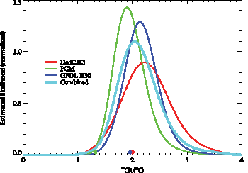
Figure 9.21. Probability distributions of TCR (expressed as warming at the time of CO2 doubling), as constrained by observed 20th-century temperature change, for the HadCM3( Table 8.1 ,red), PCM( Table 8.1 ,green) and GFDL R30 ( Delworth et al., 2002 [JoC, MoS, SRC] , blue) models. The average of the PDFs derived from each model is shown in turquoise. Coloured circles show each model’s TCR. (After Stott et al., 2006c [JoC, MoS, SRC] ).
9.6.3 Estimates of Climate Sensitivity Based on Palaeoclimatic Data
The palaeoclimate record offers a range of opportunities to assess the response of climate models to changes in external forcing. This section discusses estimates from both the palaeoclimatic record of the last millennium, and from the climate of the LGM. The latter gives a different perspective on feedbacks than anticipated with greenhouse warming, and thus provides a test bed for the physics in climate models. There also appears to be a likely positive relationship between temperature and CO2 prior to the 650 kyr period covered by ice core measurements of CO2 ( Section 6.3 ).
As with analyses of the instrumental record discussed in Section 9.6.2 ,some studies using palaeoclimatic data have also estimated PDFs for ECS by varying model parameters. Inferences about ECS made through direct comparisons between radiative forcing and climate response, without using climate models, show large uncertainties since climate feedbacks, and thus sensitivity, may be different for different climatic background states and for different seasonal characteristics of forcing (e.g., Montoya et al., 2000 [PoC, JoC, MoS] ). Thus, sensitivity to forcing during these periods cannot be directly compared to that for atmospheric CO2 doubling.
9.6.3.1 Estimates of Climate Sensitivity Based on Data for the Last Millennium
The relationship between forcing and response based on a long time horizon can be studied using palaeoclimatic reconstructions of temperature and radiative forcing, particularly volcanism and solar forcing, for the last millennium. However, both forcing and temperature reconstructions are subject to large uncertainties( Chapter6 ). To account for the uncertainty in reconstructions, Hegerl et al. 2006a [NPR, PoC, JoC, SRC] ) use several proxy data reconstructions of NH extratropical temperature for the past millennium ( Briffa et al., 2001 [PoC, JoC, ARC] ; Esper et al., 2002 [PoC, JoC, ARC] ; Mann and Jones, 2003 [PoC, JoC, ARC] ; Hegerl et al., 2007 [JoC, SRC, 2007] ) to constrain ECS estimates for the pre-industrial period up to 1850 . This study used a large ensemble of simulations of the last millennium performed with an energy balance model forced with reconstructions of volcanic ( Crowley, 2000 [PoC, JoC] , updated), solar ( Lean et al., 2002 [JoC, MoS, ARC] ) and greenhouse gas forcing (see Section 9.3.3 for results on the detection of these external influences). Their estimated PDFs for ECS incorporate an estimate of uncertainty in the overall amplitude (including an attempt to account for uncertainty in efficacy), but not the time evolution, of volcanic and solar forcing. They also attempt to account for uncertainty in the amplitude of reconstructed temperatures in one reconstruction ( Hegerl et al., 2007 [JoC, SRC, 2007] ), and assess the sensitivity of their results to changes in amplitude for others. All reconstructions combined yield a median climate sensitivity of 3.4°C and a 5 to 95% range of 1.2°C to 8.6°C( Figure 9.20 ). Reconstructions with a higher amplitude of past climate variations (e.g., Esper et al., 2002 [PoC, JoC, ARC] ; Hegerl et al., 2007 [JoC, SRC, 2007] ) are found to support higher ECS estimates than reconstructions with lower amplitude (e.g., Mann and Jones, 2003 [PoC, JoC, ARC] ). Note that the constraint on ECS originates mainly from low-frequency temperature variations associated with changes in the frequency and intensity of volcanism which lead to a highly significant detection of volcanic response( Section 9.3.3 )in all records used in the study.
The results of Andronova et al. 2004 [PoC, JoC, SRC] ) are broadly consistent with these estimates. Andronova et al. 2004 [PoC, JoC, SRC] ) demonstrate that climate sensitivities in the range of 2.3°C to 3.4°C yield reasonable simulations of both the NH mean temperature from 1500 onward when compared to the Mann and Jones 2003 [PoC, JoC, ARC] ) reconstruction, and for the instrumental period. The agreement is less good for reconstructed SH temperature, where reconstructions are substantially more uncertain( Chapter6 ).
Rind et al. 2004 [JoC, MoS, SRC] ) studied the period from about 1675 to 1715 to attempt a direct estimate of climate sensitivity. This period has reduced radiative forcing relative to the present due to decreased solar radiation, decreased greenhouse gas and possibly increased volcanic forcing( Section 9.2.1.3 ). Different NH temperature reconstructions( Figure 6.10 )have a wide range of cooling estimates relative to the late 20th century that is broadly reproduced by climate model simulations. While climate in this cold period may have been close to radiative balance ( Rind et al., 2004 [JoC, MoS, SRC] ), some of the forcing during the present period is not yet realised in the system (estimated as 0.85 Wm–2 ;Hansen et al., 2005 [JoC, ARC] ). Thus, ECS estimates based on a comparison between radiative forcing and climate response are subject to large uncertainties, but are broadly similar to estimates discussed above. Again, reconstructions with stronger cooling in this period imply higher climate sensitivities than those with weaker cooling (results updated from Rind et al., 2004 [JoC, MoS, SRC] ).
9.6.3.2 Inferences About Climate Sensitivity Based on the Last Glacial Maximum
The LGM is one of the key periods used to estimate ECS ( Hansen et al., 1984 [NPR, ARC] ; Lorius et al., 1990 [JoC, MoS] ; Hoffert and Covey, 1992 [JoC, ARC] ), since it represents a quasi-equilibrium climate response to substantially altered boundary conditions. When forced with changes in greenhouse gas concentrations and the extent and height of ice sheet boundary conditions, AOGCMs or EMICs identical or similar to those used for 20th- and 21st-century simulations produce a 3.3°C to 5.1°C cooling for this period in response to radiative perturbations of 4.6 to 7.2 Wm–2 (Sections 6.4.1.3 ;see also Section 9.3.2 ;see also Masson-Delmotte et al., 2006 [JoC, MoS, SRC] ). The simulated cooling in the tropics ranges from 1.7°C to 2.4°C. The ECS of the models used in PMIP2 ranges from 2.3°C to 3.7°C( Table 8.2 ), and there is some tendency for models with larger sensitivity to produce larger tropical cooling for the LGM, but this relationship is not very tight. Comparison between simulated climate change and reconstructed climate is affected by substantial uncertainties in forcing and data( Chapter6 and Section 9.2.1.3 ). For example, the PMIP2 forcing does not account for changes in mineral dust, since the level of scientific understanding for this forcing is very low( Figure 6.5 ). The range of simulated temperature changes is also affected by differences in the radiative influence of the ice-covered regions in different models ( Taylor et al., 2000 [NPR, MoS, ARC] ). Nevertheless, the PMIP2 models simulate LGM climate changes that are approximately consistent with proxy information( Chapter6 ).
Recent studies ( Annan et al., 2005 [MoS, ARC] ; Schneider von Deimling et al., 2006 [PoC, JoC, MoS, ARC] ) attempt to estimate the PDF of ECS from ensemble simulations of the LGM by systematically exploring model uncertainty. Both studies investigate the relationship between climate sensitivity and LGM tropical SSTs, which are influenced strongly by CO2 changes. In a perturbed physics ensemble, Schneider von Deimling et al. 2006 [PoC, JoC, MoS, ARC] ) vary 11 ocean and atmospheric parameters in a 1,000-member ensemble simulation of the LGM with the CLIMBER-2 EMIC( Table 8.3 ). They find a close relationship between ECS and tropical SST cooling in their model, implying a 5 to 95% range of ECS of 1.2°C to 4.3°C when attempting to account for model parameter, forcing and palaeoclimate data uncertainties. Similar constraints on climate sensitivity are found when proxy reconstructions of LGM antarctic temperatures are used instead of tropical SSTs ( Schneider von Deimling et al., 2006 [PoC, JoC, MoS, ARC] ). In contrast, Annan et al. 2005 [MoS, ARC] ) use a perturbed physics ensemble based on a low-resolution version of the atmospheric component of the MIROC3.2 model, perturbing a range of model parameters over prior distributions determined from the ability of the model to reproduce seasonal mean climate in a range of climate variables. They find a best-fit sensitivity of about 4.5°C, and their results suggest that sensitivities in excess of 6°C are unlikely given observational estimates of LGM tropical cooling and the relationship between tropical SST and sensitivity in their model. Since the perturbed physics ensemble based on that atmospheric model does not produce sensitivities less than 4°C, this result cannot provide a lower limit or a PDF for ECS.
The discrepancy between the inferred upper limits in the two studies probably arises from both different radiative forcing and structural differences between the models used. Forcing from changes in vegetation cover and dust is not included in the simulations done by Annan et al. 2005 [MoS, ARC] ), which according to Schneider von Deimling et al. 2006 [PoC, JoC, MoS, ARC] ) would reduce the Annan et al. ECS estimates and yield better agreement between the results of the two studies. However, the effect of these forcings and their interaction with other LGM forcings is very uncertain, limiting confidence in such estimates of their effect( Figure 6.5 ). Structural differences in models are also likely to play a role. The Annan et al. 2005 [MoS, ARC] ) estimate shows a weaker association between simulated tropical SST changes and ECS than the Schneider von Deimling et al. 2006 [PoC, JoC, MoS, ARC] ) result. Since Annan et al. use a mixed-layer ocean model, and Schneider von Deimling a simplified ocean model, both models may not capture the full ocean response affecting tropical SSTs. The atmospheric model used in Schneider von Deimling is substantially simpler than that used in the Annan et al. 2005 [MoS, ARC] ) study. Overall, estimates of climate sensitivity from the LGM are broadly consistent with other estimates of climate sensitivity derived, for example, from the instrumental period.
9.6.4 Summary of Observational Constraints for Climate Sensitivity
Any constraint of climate sensitivity obtained from observations must be interpreted in light of the underlying assumptions. These assumptions include (i) the choice of prior distribution for each of the model parameters( Section 9.6.1 and Supplementary Material, Appendix 9.B ), including the parameter range explored, (ii) the treatment of other parameters that influence the estimate, such as effective ocean diffusivity, and (iii) the methods used to account for uncertainties, such as structural and forcing uncertainties, that are not represented by the prior distributions. Neglecting important sources of uncertainty in these estimates will result in overly narrow ranges that overstate the certainty with which the ECS or TCR is known. Errors in assumptions about forcing or model response will also result in unrealistic features of model simulations, which can result in erroneous modes (peak probabilities) and shapes of the PDF. On the other hand, using less than all available information will yield results that are less constrained than they could be under optimal use of available data.
While a variety of important uncertainties (e.g., radiative forcing, mixing of heat into the ocean) have been taken into account in most studies( Table 9.3 ), some caveats remain. Some processes and feedbacks might be poorly represented or missing, particularly in simple and many intermediate complexity models. Structural uncertainties in the models, for example, in the representation of cloud feedback processes( Chapter8 )or the physics of ocean mixing, will affect results for climate sensitivity and are very difficult to quantify. In addition, differences in efficacy between forcings are not directly represented in simple models, so they may affect the estimate (e.g., Tett et al., 2007 [JoC, MoS, SRC, 2007] ), although this uncertainty may be folded into forcing uncertainty (e.g., Hegerl et al., 2003 [JoC, SRC] , 2007 ). The use of a single value for the ECS further assumes that it is constant in time. However, some authors (e.g., Senior and Mitchell, 2000 [JoC, SRC] ; Boer and Yu, 2003 [JoC] ) have shown that ECS varies in time in the climates simulated by their models. Since results from instrumental data and the last millennium are dominated primarily by decadal- to centennial-scale changes, they will therefore only represent climate sensitivity at an equilibrium that is not too far from the present climate. There is also a small uncertainty in the radiative forcing due to atmospheric CO2 doubling (<10%; see Chapter2 ), which is not accounted for in most studies that derive observational constraints on climate sensitivity.
Despite these uncertainties, which are accounted for to differing degrees in the various studies, confidence is increased by the similarities between individual ECS estimates( Figure 9.20 ). Most studies find a lower 5% limit of between 1°C and 2.2°C, and studies that use information in a relatively complete manner generally find a most likely value between 2°C and 3°C( Figure 9.20 ). Constraints on the upper end of the likely range of climate sensitivities are also important, particularly for probabilistic forecasts of future climate with constant radiative forcing. The upper 95% limit for ECS ranges from 5°C to 10°C, or greater in different studies depending upon the approach taken, the number of uncertainties included and specific details of the prior distribution that was used. This wide range is largely caused by uncertainties and nonlinearities in forcings and response. For example, a high sensitivity is difficult to rule out because a high aerosol forcing could nearly cancel greenhouse gas forcing over the 20th century. This problem can be addressed, at least to some extent, if the differences in the spatial and temporal patterns of response between aerosol and greenhouse gas forcing are used for separating these two responses in observations (as, for example, in Gregory et al., 2002a [JoC, MoS, SRC] ; Harvey and Kaufmann, 2002 [JoC, MoS] ; Frame et al., 2005 [JoC, MoS] ). In addition, nonlinearities in the response to transient forcing make it more difficult to constrain the upper limit on ECS based on observed transient forcing responses ( Frame et al., 2005 [JoC, MoS] ). The TCR, which may be more relevant for near-term climate change, is easier to constrain since it relates more linearly to observables. For the pre-instrumental part of the last millennium, uncertainties in temperature and forcing reconstructions, and the nonlinear connection between ECS and the response to volcanism, prohibit tighter constraints. Estimates of climate sensitivity based on the ability of climate models to reproduce climatic conditions of the LGM broadly support the ranges found from the instrumental period, although a tight constraint is also difficult to obtain from this period alone because of uncertainties in tropical temperature changes, forcing uncertainties and the effect of structural model uncertainties. In addition, the number of studies providing estimates of PDFs from palaeoclimatic data, using independent approaches and complementary sources of proxy data, are limited.
Thus, most studies that use a simple uniform prior distribution of ECS are not able to exclude values beyond the traditional IPCC First Assessment Report range of 1.5°C to 4.5°C ( IPCC, 1990 [NPR] ). However, considering all available evidence on ECS together provides a stronger constraint than individual lines of evidence. Bayesian methods can be used to incorporate multiple lines of evidence to sharpen the posterior distribution of ECS, as in Annan and Hargreaves 2006 [JoC, MoS, ARC] and Hegerl et al. 2006a [NPR, PoC, JoC, SRC] Annan and Hargreaves 2006 [JoC, MoS, ARC] ) demonstrate that using three lines of evidence, namely 20th-century warming, the response to individual volcanic eruptions and the LGM response, results in a tighter estimate of ECS, with a probability of less than 5% that ECS exceeds 4.5°C. The authors find a similar constraint using five lines of evidence under more conservative assumptions about uncertainties (adding cooling during the Little Ice Age and studies based on varying model parameters to match climatological means, see Box 10.2 ). However, as discussed in Annan and Hargreaves 2006 [JoC, MoS, ARC] ), combining multiple lines of evidence may produce overly confident estimates unless every single line of evidence is entirely independent of others, or dependence is explicitly taken into account. Hegerl et al. 2006a [NPR, PoC, JoC, SRC] ) argue that instrumental temperature change during the second half of the 20th century is essentially independent of the palaeoclimate record of the last millennium and of the instrumental data from the first half of the 20th century that is used to calibrate the palaeoclimate records. Hegerl et al. 2006a [NPR, PoC, JoC, SRC] ) therefore base their prior probability distribution for the climate sensitivity on results from the late 20th century ( Frame et al., 2005 [JoC, MoS] ), which reduces the 5 to 95% ECS range from all proxy reconstructions analysed to 1.5°C to 6.2°C compared to the previous range of 1.2°C to 8.6°C. Both results demonstrate that independent estimates, when properly combined in a Bayesian analysis, can provide a tighter constraint on climate sensitivity, even if they individually provide only weak constraints. These studies also find a 5% lower limit of 1.5°C or above, consistent with several studies based on the 20th-century climate change alone ( Knutti et al., 2002 [PoC, JoC, MoS, SRC] ; Forest et al., 2006 [JoC, MoS, ARC] ) and estimates that greenhouse warming contributes substantially to observed temperature changes( Section 9.4.1.4 ).
Overall, several lines of evidence strengthen confidence in present estimates of ECS, and new results based on objective analyses make it possible to assign probabilities to ranges of climate sensitivity previously assessed from expert opinion alone. This represents a significant advance. Results from studies of observed climate change and the consistency of estimates from different time periods indicate that ECS is very likely larger than 1.5°C with a most likely value between 2°C and 3°C. The lower bound is consistent with the view that the sum of all atmospheric feedbacks affecting climate sensitivity is positive. Although upper limits can be obtained by combining multiple lines of evidence, remaining uncertainties that are not accounted for in individual estimates (such as structural model uncertainties) and possible dependencies between individual lines of evidence make the upper 95% limit of ECS uncertain at present. Nevertheless, constraints from observed climate change support the overall assessment that the ECS is likely to lie between 2°C and 4.5°C with a most likely value of approximately 3°C( Box 10.2 ).
9.7 Combining Evidence of Anthropogenic Climate Change
The widespread change detected in temperature observations of the surface (Sections 9.4.1 , 9.4.2 , 9.4.3 ), free atmosphere( Section 9.4.4 )and ocean( Section 9.5.1 ), together with consistent evidence of change in other parts of the climate system( Section 9.5 ), strengthens the conclusion that greenhouse gas forcing is the dominant cause of warming during the past several decades. This combined evidence, which is summarised in Table 9.4 ,is substantially stronger than the evidence that is available from observed changes in global surface temperature alone( Figure 3.6 ).
The evidence from surface temperature observations is strong: The observed warming is highly significant relative to estimates of internal climate variability which, while obtained from models, are consistent with estimates obtained from both instrumental data and palaeoclimate reconstructions. It is extremely unlikely (<5%) that recent global warming is due to internal variability alone such as might arise from El Niño( Section 9.4.1 ). The widespread nature of the warming (Figures 3.9 and 9.6 )reduces the possibility that the warming could have resulted from internal variability. No known mode of internal variability leads to such widespread, near universal warming as has been observed in the past few decades. Although modes of internal variability such as El Niño can lead to global average warming for limited periods of time, such warming is regionally variable, with some areas of cooling (Figures 3.27 and 3.28 ). In addition, palaeoclimatic evidence indicates that El Niño variability during the 20th century is not unusual relative to earlier periods( Section 9.3.3.2 ; Chapter6 ). Palaeoclimatic evidence suggests that such a widespread warming has not been observed in the NH in at least the past 1.3 kyr ( Osborn and Briffa, 2006 [PoC, JoC, ARC] ), further strengthening the evidence that the recent warming is not due to natural internal variability. Moreover, the response to anthropogenic forcing is detectable on all continents individually except Antarctica, and in some sub-continental regions. Climate models only reproduce the observed 20th-century global mean surface warming when both anthropogenic and natural forcings are included( Figure 9.5 ). No model that has used natural forcing only has reproduced the observed global mean warming trend or the continental mean warming trends in all individual continents (except Antarctica) over the second half of the 20th century. Detection and attribution of external influences on 20th-century and palaeoclimatic reconstructions, from both natural and anthropogenic sources( Figure 9.4 and Table 9.4 ), further strengthens the conclusion that the observed changes are very unusual relative to internal climate variability.
The energy content change associated with the observed widespread warming of the atmosphere is small relative to the energy content change of the ocean, and also smaller than that associated with other components such as the cryosphere. In addition, the solid Earth also shows evidence for warming in boreholes ( Huang et al., 2000 [JoC, ARC] ; Beltrami et al., 2002 [JoC, ARC] ; Pollack and Smerdon, 2004 [JoC, ARC] ). It is theoretically feasible that the warming of the near surface could have occurred due to a reduction in the heat content of another component of the system. However, all parts of the cryosphere (glaciers, small ice caps, ice sheets and sea ice) have decreased in extent over the past half century, consistent with anthropogenic forcing( Section 9.5.5 , Table 9.4 ), implying that the cryosphere consumed heat and thus indicating that it could not have provided heat for atmospheric warming. More importantly, the heat content of the ocean (the largest reservoir of heat in the climate system) also increased, much more substantially than that of the other components of the climate system( Figure 5.4 ;Hansen et al., 2005 [JoC, ARC] ; Levitus et al., 2005 [JoC, ARC] ). The warming of the upper ocean during the latter half of the 20th century was likely due to anthropogenic forcing ( Barnett et al., 2005 [JoC] ; Section 9.5.1.1 ; Table 9.4 ). While the statistical evidence in this research is very strong that the warming cannot be explained by ocean internal variability as estimated by two different climate models, uncertainty arises since there are discrepancies between estimates of ocean heat content variability from models and observations, although poor sampling of parts of the World Ocean may explain this discrepancy. However, the spatial pattern of ocean warming with depth is very consistent with heating of the ocean resulting from net positive radiative forcing, since the warming proceeds downwards from the upper layers of the ocean and there is deeper penetration of heat at middle to high latitudes and shallower penetration at low latitudes ( Barnett et al., 2005 [JoC] ; Hansen et al., 2005 [JoC, ARC] ). This observed ocean warming pattern is inconsistent with a redistribution of heat between the surface and the deep ocean.
Thus, the evidence appears to be inconsistent with the ocean or land being the source of the warming at the surface. In addition, simulations forced with observed SST changes cannot fully explain the warming in the troposphere without increases in greenhouse gases (e.g., Sexton et al., 2001 [JoC, SRC] ), further strengthening the evidence that the warming does not originate from the ocean. Further evidence for forced changes arises from widespread melting of the cryosphere( Section 9.5.5 ), increases in water vapour in the atmosphere( Section 9.5.4.1 )and changes in top-of-the atmosphere radiation that are consistent with changes in forcing.
The simultaneous increase in energy content of all the major components of the climate system and the pattern and amplitude of warming in the different components, together with evidence that the second half of the 20th century was likely the warmest in 1.3 kyr( Chapter6 )indicate that the cause of the warming is extremely unlikely to be the result of internal processes alone. The consistency across different lines of evidence makes a strong case for a significant human influence on observed warming at the surface. The observed rates of surface temperature and ocean heat content change are consistent with the understanding of the likely range of climate sensitivity and net climate forcings. Only with a net positive forcing, consistent with observational and model estimates of the likely net forcing of the climate system (as used in Figure 9.5 ), is it possible to explain the large increase in heat content of the climate system that has been observed( Figure 5.4 ).
Table 9.4. A synthesis of climate change detection results: (a) surface and atmospheric temperature evidence and (b) evidence from other variables. Note that our likelihood assessments are reduced compared to individual detection studies in order to take into account remaining uncertainties (see Section 9.1.2 ), such as forcing and model uncertainty not directly accounted for in the studies. The likelihood assessment is indicated in percentage terms, in parentheses where the term is not from the standard IPCC likelihood levels.
a)
b)
| Result | Region | Likelihood | Factors contributing to likelihood assessment |
|---|---|---|---|
| Surface temperature | |||
| Warming during the past half century cannot be explained without external radiative forcing | Global | Extremely likely (>95%) | Anthropogenic change has been detected in surface temperature with very high significance levels (less than 1% error probability). This conclusion is strengthened by detection of anthropogenic change in the upper ocean with high significance level. Upper ocean warming argues against the surface warming being due to natural internal processes. Observed change is very large relative to climate-model simulated internal variability. Surface temperature variability simulated by models is consistent with variability estimated from instrumental and palaeorecords. Main uncertainty from forcing and internal variability estimates (Sections 9.4.1.2 , 9.4.1.4 , 9.5.1.1 , 9.3.3.2 , 9.7 ). |
| Warming during the past half century is not solely due to known natural causes | Global | Very Likely | This warming took place at a time when non-anthropogenic external factors would likely have produced cooling. The combined effect of known sources of forcing would have been extremely likely to produce a warming. No climate model that has used natural forcing only has reproduced the observed global warming trend over the 2nd half of the 20th century. Main uncertainties arise from forcing, including solar, model-simulated responses and internal variability estimates (Sections 2.9.2 , 9.2.1 , 9.4.1.2 , 9.4.1.4 ;Figures 9.5 , 9.6 , 9.9 ). |
| Greenhouse gas forcing has been the dominant cause of the observed global warming over the last 50 years. | Global | Very likely | All multi-signal detection and attribution studies attribute more warming to greenhouse gas forcing than to a combination of all other sources considered, including internal variability, with a very high significance. This conclusion accounts for observational, model and forcing uncertainty, and the possibility that the response to solar forcing could be underestimated by models. Main uncertainty from forcing and internal variability estimates( Section 9.4.1.4 ; Figure 9.9 ). |
| Increases in greenhouse gas concentrations alone would have caused more warming than observed over the last 50 years because volcanic and anthropogenic aerosols have offset some warming that would otherwise have taken place. | Global | Likely | Estimates from different analyses using different models show consistently more warming than observed over the last 50 years at the 5% significance level. However, separation of the response to non-greenhouse gas (particularly aerosol) forcing from greenhouse gas forcing varies between models( Section 9.4.1.4 ; Figure 9.9 ). |
| There has been a substantial anthropogenic contribution to surface temperature increases in every continent except Antarctica since the middle of the 20th century | Africa, Asia, Australia, Europe, North America and South America | Likely | Anthropogenic change has been estimated using detection and attribution methods on every individual continent (except Antarctica). Greater variability compared to other continental regions makes detection more marginal in Europe. No climate model that used natural forcing only reproduced the observed continental mean warming trend over the second half of the 20th century. Uncertainties arise because sampling effects result in lower signal-to-noise ratio at continental than at global scales. Separation of the response to different forcings is more difficult at these spatial scales( Section 9.4.2 ; FAQ 9.2 ,Figure 1). |
| Early 20th-century warming is due in part to external forcing. | Global | Very Likely | Anumber of studies detect the influence of external forcings on early 20th-century warming, including a warming from anthropogenic forcing. Both natural forcing and response are uncertain, and different studies find different forcings dominant. Some studies indicate that internal variability could have made a large contribution to early 20th-century warming. Some observational uncertainty in early 20th-century trend (Sections 9.3.3.2 , 9.4.1.4 ;Figures 9.4 , 9.5 ). |
| Result | Region | Likelihood | Factors contributing to likelihood assessment |
| Surface temperature | |||
| Pre-industrial temperatures were influenced by natural external forcing (period studied is past 7 centuries) | NH (mostly extratropics) | Very Likely | Detection studies indicate that external forcing explains a substantial fraction of inter-decadal variability in NH temperature reconstructions. Simulations in response to estimates of pre-industrial forcing reproduce broad features of reconstructions. Substantial uncertainties in reconstructions and past forcings are unlikely to lead to a spurious agreement between temperature reconstructions and forcing reconstructions as they are derived from independent proxies( Section 9.3.3 ;Figures 9.4 , 6.13 ). |
| Temperature extremes have changed due to anthropogenic forcing | NH land areas and Australia combined. | Likely | Arange of observational evidence indicates that temperature extremes are changing. An anthropogenic influence on the temperatures of the 1, 5, 10 and 30 warmest nights, coldest days and coldest nights annually has been formally detected and attributed in one study, but observed change in the temperature of the warmest day annually is inconsistent with simulated change. The detection of changes in temperature extremes is supported by other comparisons between models and observations. Model uncertainties in changes in temperature extremes are greater than for mean temperatures and there is limited observational coverage and substantial observational uncertainty( Section 9.4.3 ). |
| Free atmosphere changes | |||
| Tropopause height increases are detectable and attributable to anthropogenic forcing (latter half of the 20th century) | Global | Likely | There has been robust detection of anthropogenic influence on increasing tropopause height. Simulated tropopause height increases result mainly from greenhouse gas increases and stratospheric ozone decreases. Detection and attribution studies rely on reanalysis data, which are subject to inhomogeneities related to differing availability and quality of input data, although tropopause height increases have also been identified in radiosonde observations. Overall tropopause height increases in recent model and one reanalysis (ERA-40) appear to be driven by similar large-scale changes in atmospheric temperature, although errors in tropospheric warming and stratospheric cooling could lead to partly spurious agreement in other data sets( Section 9.4.4.2 ; Figure 9.14 ). |
| Tropospheric warming is detectable and attributable to anthropogenic forcing (latter half of the 20th century) | Global | Likely | There has been robust detection and attribution of anthropogenic influence on tropospheric warming, which does not depend on including stratospheric cooling in the fingerprint pattern of response. There are observational uncertainties in radiosonde and satellite records. Models generally predict a relative warming of the free troposphere compared to the surface in the tropics since 1979, which is not seen in the radiosonde record (possibly due to uncertainties in the radiosonde record) but is seen in one version of the satellite record, although not others( Section 9.4.4 ). |
| Simultaneous tropospheric warming and stratospheric cooling due to the influence of anthropogenic forcing has been observed (latter half of the 20th century) | Global | Very Likely | Simultaneous warming of the troposphere and cooling of the stratosphere due to natural factors is less likely than warming of the troposphere or cooling of the stratosphere alone. Cooling of the stratosphere is in part related to decreases in stratospheric ozone. Modelled and observational uncertainties as discussed under entries for tropospheric warming with additional uncertainties due to stratospheric observing systems and the relatively poor representations of stratospheric processes and variability in climate models( Section 9.4.4 ). |
| Result | Region | Likelihood | Factors contributing to likelihood assessment |
|---|---|---|---|
| Ocean changes | |||
| Anthropogenic forcing has warmed the upper several hundred metres of the ocean during the latter half of the 20th century | Global (but with limited sampling in some regions) | Likely | Robust detection and attribution of anthropogenic fingerprint from three different models in ocean temperature changes, and in ocean heat content data, suggests high likelihood, but observational and modelling uncertainty remains. 20th-century simulations with MMD models simulate comparable ocean warming to observations only if anthropogenic forcing is included. Simulated and observed variability appear inconsistent, either due to sampling errors in the observations or under-simulated internal variability in the models. Limited geographical coverage in some ocean basins( Section 9.5.1.1 ; Figure 9.15 ). |
| Anthropogenic forcing contributed to sea level rise during the latter half 20th century | Global | Very likely | Natural factors alone do not satisfactorily explain either the observed thermal expansion of the ocean or the observed sea level rise. Models including anthropogenic and natural forcing simulate the observed thermal expansion since 1961 reasonably well. Anthropogenic forcing dominates the surface temperature change simulated by models, and has likely contributed to the observed warming of the upper ocean and widespread glacier retreat. It is very unlikely that the warming during the past half century is due only to known natural causes. It is therefore very likely that anthropogenic forcing contributed to sea level rise associated with ocean thermal expansion and glacier retreat. However, it remains difficult to estimate the anthropogenic contribution to sea level rise because suitable studies quantifying the anthropogenic contribution to sea level rise and glacier retreat are not available, and because the observed sea level rise budget is not closed( Table 9.2 ; Section 9.5.2 ). |
| Circulation | |||
| Sea level pressure shows a detectable anthropogenic signature during the latter half of the 20th century | Global | Likely | Changes of similar nature are observed in both hemispheres and are qualitatively, but not quantitatively consistent with model simulations. Uncertainty in models and observations. Models underestimate the observed NH changes for reasons that are not understood, based on a small number of studies. Simulated response to 20th century forcings is consistent with observations in SH if effect of stratospheric ozone depletion is included( Section 9.5.3.4 ; Figure 9.16 ). |
| Anthropogenic forcing contributed to the increase in frequency of the most intense tropical cyclones since the 1970s | Tropical regions | More likely than not (>50%) | Recent observational evidence suggests an increase in frequency of intense storms. Increase in intensity is consistent with theoretical expectations. Large uncertainties due to models and observations. Modelling studies generally indicate a reduced frequency of tropical cyclones in response to enhanced greenhouse gas forcing, but an increase in the intensity of the most intense cyclones. Observational evidence, which is affected by substantial inhomogeneities in tropical cyclone data sets for which corrections have been attempted, suggests that increases in cyclone intensity since the 1970s are associated with SST and atmospheric water vapour increases( Section 3.8.3 , Box 3.5 and Section 9.5.2.6). |
| Precipitation, Drought, Runoff | |||
| Volcanic forcing influences total rainfall | Global land areas | More likely than not (>50%) | Model response detectable in observations for some models and result supported by theoretical understanding. However, uncertainties in models, forcings and observations. Limited observational sampling, particularly in the SH( Section 9.5.4.2 ; Figure 9.18 ). |
| Increases in heavy rainfall are consistent with anthropogenic forcing during latter half 20th century | Global land areas (limited sampling) | More likely than not (>50%) | Observed increases in heavy precipitation appear to be consistent with expectations of response to anthropogenic forcing. Models may not represent heavy rainfall well; observations suffer from sampling inadequacies( Section 9.5.4.2 ). |
| Result | Region | Likelihood | Factors contributing to likelihood assessment |
| Precipitation, Drought, Runoff | |||
| Increased risk of drought due to anthropogenic forcing during latter half 20th century | Global land areas | More likely than not (>50%) | One detection study has identified an anthropogenic fingerprint in a global Palmer Drought Severity Index data set with high significance, but the simulated response to anthropogenic and natural forcing combined is weaker than observed, and the model appears to have less inter-decadal variability than observed. Studies of some regions indicate that droughts in those regions are linked either to SST changes that, in some instances, may be linked to anthropogenic aerosol forcing (e.g., Sahel) or to a circulation response to anthropogenic forcing (e.g., southwest Australia). Models, observations and forcing all contribute uncertainty( Section 9.5.3.2 ). |
| Cryosphere | |||
| Anthropogenic forcing has contributed to reductions in NH sea ice extent during the latter half of the 20th century | Arctic | Likely | The observed change is qualitatively consistent with model-simulated changes for most models and expectation of sea ice melting under arctic warming. Sea ice extent change detected in one study. The model used has some deficiencies in arctic sea ice annual cycle and extent. The conclusion is supported by physical expectations and simulations with another climate model. Change in SH sea ice probably within range explained by internal variability( Section 9.5.5.1 ). |
| Anthropogenic forcing has contributed to widespread glacier retreat during the 20th century | Global | Likely | Observed changes are qualitatively consistent with theoretical expectations and temperature detection. Anthropogenic contribution to volume change difficult to estimate. Few detection and attribution studies, but retreat in vast majority of glaciers consistent with expected reaction to widespread warming( Section 9.5.5.3 ). |
Appendix 9.A: Methods Used to Detect Externally Forced Signals
Appendix 9.A: Methods Used to Detect Externally Forced Signals
This appendix very briefly reviews the statistical methods that have been used in most recent detection and attribution work. Standard ‘frequentist’ methods (methods based on the relative frequency concept of probability) are most often used, but there is also increasing use of Bayesian methods of statistical inference. The following sections briefly describe the optimal fingerprinting technique followed by a short discussion on the differences between the standard and Bayesian approaches to statistical inferences that are relevant to detection and attribution.
9.A.1 Optimal Fingerprinting
Optimal fingerprinting is generalised multivariate regression adapted to the detection of climate change and the attribution of change to externally forced climate change signals ( Hasselmann, 1979 [NPR] , 1997; Allen and Tett, 1999 [JoC, MoS, SRC] ). The regression model has the form y= Xa +u,where vector y is a filtered version of the observed record, matrix X contains the estimated response patterns to the external forcings (signals) that are under investigation, a is a vector of scaling factors that adjusts the amplitudes of those patterns and u represents internal climate variability. Vector u is usually assumed to be a Gaussian random vector with covariance matrix C.Vector a is estimated with â = (XTC-1X)-1XTC-1y,which is equivalent to (TX)-1XTỹ,where matrix X and vector ỹ represent the signal patterns and observations after normalisation by the climate’s internal variability. This normalisation, standard in linear regression, is used in most detection and attribution approaches to improve the signal-to-noise ratio (see, e.g., Hasselmann, 1979 [NPR] ; Allen and Tett, 1999 [JoC, MoS, SRC] ; Mitchell et al., 2001 [NPR] ).
The matrix X typically contains signals that are estimated with either an AOGCM, an AGCM (see Sexton et al., 2001 [JoC, SRC] , 2003 ) or a simplified climate model such as an EBM. Because AOGCMs simulate natural internal variability as well as the response to specified anomalous external forcing, AOGCM-simulated climate signals are typically estimated by averaging across an ensemble of simulations (for a discussion of optimal ensemble size and composition, see Sexton et al., 2003 [PoC, JoC, MoS, SRC] ). If an observed response is to be attributed to anthropogenic influence, X should at a minimum contain separate natural and anthropogenic responses. In order to relax the assumption that the relative magnitudes of the responses to individual forcings are correctly simulated, X may contain separate responses to all the main forcings, including greenhouse gases, sulphate aerosol, solar irradiance changes and volcanic aerosol. The vector a accounts for possible errors in the amplitude of the external forcing and the amplitude of the climate model’s response by scaling the signal patterns to best match the observations.
Fitting the regression model requires an estimate of the covariance matrix C (i.e., the internal variability), which is usually obtained from unforced variation simulated by AOGCMs (e.g., from long control simulations) because the instrumental record is too short to provide a reliable estimate and may be affected by external forcing. Atmosphere-Ocean General Circulation Models may not simulate natural internal climate variability accurately, particularly at small spatial scales, and thus a residual consistency test ( Allen and Tett, 1999 [JoC, MoS, SRC] ) is typically used to assess the model-simulated variability at the scales that are retained in the analysis. To avoid bias ( Hegerl et al., 1996 [JoC, SRC] , 1997 ), uncertainty in the estimate of the vector of scaling factors a is usually assessed with a second, statistically independent estimate of the covariance matrix C which is ordinarily obtained from an additional, independent sample of simulated unforced variation.
Signal estimates are obtained by averaging across an ensemble of forced climate change simulations, but contain remnants of the climate’s natural internal variability because the ensembles are finite. When ensembles are small or signals weak, these remnants may bias ordinary least-squares estimates of a downward. This is avoided by estimating a with the total least-squares algorithm ( Allen and Stott 2003 [JoC, MoS, SRC] ).
9.A.2 Methods of Inference
Detection and attribution questions are assessed through a combination of physical reasoning (to determine, for example, by assessing consistency of possible responses, whether other mechanisms of change not included in the climate model could plausibly explain the observed change) and by evaluating specific hypotheses about the scaling factors contained in a.Most studies evaluate these hypotheses using standard frequentist methods ( Hasselmann, 1979 [NPR] , 1997; Hegerl et al., 1997 [JoC, SRC] ; Allen and Tett, 1999 [JoC, MoS, SRC] ). Several recent studies have also used Bayesian methods ( Hasselmann, 1998 [JoC] ; Leroy, 1998 [JoC] ; Min et al., 2004 [ARC] , 2005; Lee et al., 2005 [JoC, SRC] , 2006; Schnur and Hasselmann, 2005 [JoC] ; Min and Hense, 2006a [JoC, MoS] ,b).
In the standard approach, detection of a postulated climate change signal occurs when its amplitude in observations is shown to be significantly different from zero (i.e., when the null hypothesis HD : a=0 where 0 is a vector of zeros, is rejected) with departure from zero in the physically plausible direction. Subsequently, the second attribution requirement (consistency with a combination of external forcings and natural internal variability) is assessed with the ‘attribution consistency test’ ( Hasselmann, 1997 [JoC] ; see also Allen and Tett, 1999 [JoC, MoS, SRC] ) that evaluates the null hypothesis HA : a=1 where 1 denotes a vector of units. This test does not constitute a complete attribution assessment, but contributes important evidence to such assessments (see Mitchell et al., 2001 [NPR] ). Attribution studies usually also test whether the response to a key forcing, such as greenhouse gas increases, is distinguishable from that to other forcings, usually based on the results of multiple regression (see above) using the most important forcings simultaneously in X.If the response to a key forcing (e.g., due to greenhouse gas increases) is detected by rejecting the hypothesis that its amplitudeaGHG=0 in such a multiple regression, this provides strong attribution information because it demonstrates that the observed climate change is ‘not consistent with alternative, physically plausible explanations of recent climate change that exclude important elements of the given combination of forcings’ ( Mitchell et al., 2001 [NPR] ).
Bayesian approaches are of interest because they can be used to integrate information from multiple lines of evidence, and can incorporate independent prior information into the analysis. Essentially two approaches (described below) have been taken to date. In both cases, inferences are based on a posterior distribution that blends evidence from the observations with the independent prior information, which may include information on the uncertainty of external forcing estimates, climate models and their responses to forcing. In this way, all information that enters into the analysis is declared explicitly.
Schnur and Hasselmann 2005 [JoC] ) approach the problem by developing a filtering technique that optimises the impact of the data on the prior distribution in a manner similar to the way in which optimal fingerprints maximise the ratio of the anthropogenic signal to natural variability noise in the conventional approach. The optimal filter in the Bayesian approach depends on the properties of both the natural climate variability and model errors. Inferences are made by comparing evidence, as measured by Bayes Factors ( (Kass and Raftery, 1995 ) ), for competing hypotheses. Other studies using similar approaches include Min et al. 2004 [ARC] and Min and Hense 2006a [JoC, MoS] ,b). In contrast, Berliner et al. 2000 [JoC, ARC] and Lee et al. 2005 [JoC, SRC] ) use Bayesian methods only to make inferences about the estimate of a that is obtained from conventional optimal fingerprinting.
References
AchutaRao, K.M., et al., 2006: Variability of ocean heat uptake: Reconciling observations and models. J. Geophys. Res., 111,C05019. [JoC, MoS, ARC]
Ackerman, A.S., et al., 2000: Reduction of tropical cloudiness by soot. Science, 288,1042–1047. [JoC]
Adams, J.B., M.E. Mann, and C.M. Ammann, 2003: Proxy evidence for an El Nino-like response to volcanic forcing. Nature, 426(6964), 274–278. [PoC, JoC, MoS, SRC]
Alexander, L.V., et al., 2006: Global observed changes in daily climate extremes of temperature and precipitation. J. Geophys. Res., 111,D05109, doi:10.1029/2005JD006290. [JoC, ARC]
Allan, R.J., and T.J. Ansell, 2006: A new globally-complete monthly historical gridded mean sea level pressure data set (HadSLP2): 1850-2004. J. Clim., 19,5816–5842. [JoC, ARC]
Allen, M.R., 2003: Liability for climate change. Nature, 421,891–892. [JoC, SRC]
Allen, M.R., and S.F.B. Tett, 1999: Checking for model consistency in optimal fingerprinting. Clim. Dyn., 15,419–434. [JoC, MoS, SRC]
Allen, M.R., and W.J. Ingram, 2002: Constraints on future changes in climate and the hydrologic cycle. Nature, 419,224–232. [JoC, MoS, SRC]
Allen, M.R., and D.A. Stainforth, 2002: Towards objective probabilistic climate forecasting. Nature, 419,228–228. [JoC, MoS, SRC]
Allen, M.R., and P.A. Stott, 2003: Estimating signal amplitudes in optimal fingerprinting, Part I: Theory. Clim. Dyn., 21,477–491. [JoC, MoS, SRC]
Allen, M.R., J.A. Kettleborough, and D.A. Stainforth, 2002: Model error in weather and climate forecasting. In: ECMWF Predictability of Weather and Climate Seminar [Palmer, T.N. (ed.)]. European Centre for Medium Range Weather Forecasts, Reading, UK, http://www.ecmwf.int/publications/library/do/references/list/209. [NPR, MoS, SRC]
Allen, M.R., et al., 2000: Quantifying the uncertainty in forecasts of anthropogenic climate change. Nature, 407,617–620. [JoC, MoS, SRC]
Ammann, C.M., G.A. Meehl, W.M. Washington, and C. Zender, 2003: A monthly and latitudinally varying volcanic forcing dataset in simulations of 20th century climate. Geophys. Res. Lett., 30(12), 1657. [PoC, JoC, MoS, SRC]
Anderson, T.L., et al., 2003: Climate forcing by aerosols: A hazy picture. Science, 300,1103–1104. [JoC, MoS]
Andronova, N.G., and M.E. Schlesinger, 2000: Causes of global temperature changes during the 19th and 20th centuries. Geophys. Res. Lett., 27(14), 2137–2140. [JoC, SRC]
Andronova, N.G., and M.E. Schlesinger, 2001: Objective estimation of the probability density function for climate sensitivity. J. Geophys. Res., 106(D19), 22605–22611. [JoC, MoS, SRC]
Andronova, N.G., M.E. Schlesinger, and M.E. Mann, 2004: Are reconstructed pre-instrumental hemispheric temperatures consistent with instrumental hemispheric temperatures? Geophys. Res. Lett., 31,L12202, doi:10.1029/2004GL019658. [PoC, JoC, SRC]
Andronova, N.G., et al., 1999: Radiative forcing by volcanic aerosols from 1850 to 1994. J. Geophys. Res., 104,16807–16826. [JoC, MoS, SRC]
Andronova, N.G., et al., 2007: The concept of climate sensitivity: History and development. In: Human-Induced Climate Change: An Interdisciplinary Assessment [Schlesinger, M., et al. (eds.)]. Cambridge University Press, Cambridge, UK, in press. [NPR, SRC, 2007]
Annan, J.D., and J.C. Hargreaves, 2006: Using multiple observationally-based constraints to estimate climate sensitivity. Geophys. Res. Lett., 33,L06704, doi:10.1029/2005GL025259. [JoC, MoS, ARC]
Annan, J.D., et al., 2005: Efficiently constraining climate sensitivity with paleoclimate simulations. Scientific Online Letters on the Atmosphere, 1,181–184. [MoS, ARC]
Arblaster, J.M., and G.A. Meehl, 2006: Contributions of external forcing to Southern Annular Mode trends. J. Clim., 19,2896–2905. [JoC, MoS, ARC]
Bader, J., and M. Latif, 2003: The impact of decadal-scale Indian Ocean sea surface temperature anomalies on Sahelian rainfall and the North Atlantic Oscillation. Geophys. Res. Lett., 30(22), 2169. [JoC, ARC]
Banks, H.T., et al., 2000: Are observed decadal changes in intermediate water masses a signature of anthropogenic climate change? Geophys. Res. Lett., 27,2961–2964. [JoC]
Barnett, T.P., D.W. Pierce, and R. Schnur, 2001: Detection of anthropogenic climate change in the world’s oceans. Science, 292,270–274. [JoC, SRC]
Barnett, T.P., et al., 1999: Detection and attribution of recent climate change. Bull. Am. Meteorol. Soc., 80,2631–2659. [JoC]
Barnett, T.P., et al., 2005: Penetration of a warming signal in the world’s oceans: human impacts. Science, 309,284–287. [JoC]
Bauer, E., M. Claussen, V. Brovkin, and A. Huenerbein, 2003: Assessing climate forcings of the Earth system for the past millennium. Geophys. Res. Lett., 30(6), 1276. [JoC, MoS, ARC]
Beltrami, H., J.E. Smerdon, H.N. Pollack, and S. Huang, 2002: Continental heat gain in the global climate system. Geophys. Res. Lett., 29,1167. [JoC, ARC]
Bengtsson, L., K.I. Hodges, and E. Roechner, 2006: Storm tracks and climate change. J. Clim., 19,3518–3543. [JoC, ARC]
Berger, A., 1978: Long-term variations of caloric solar radiation resulting from the earth’s orbital elements. Quat. Res., 9,139–167. [ARC]
Berger, A., 1988: Milankovitch theory and climate. Rev. Geophys., 26,624–657. [JoC, ARC]
Berliner, L.M., R.A. Levine, and D.J. Shea, 2000: Bayesian climate change assessment. J. Clim., 13,3805–3820. [JoC, ARC]
Bertrand, C., M.F. Loutre, M. Crucifix, and A. Berger, 2002: Climate of the last millennium: a sensitivity study. Tellus, 54A(3), 221–244. [JoC, ARC]
Betts, R.A., 2001: Biogeophysical impacts of land use on present-day climate: near surface temperature and radiative forcing. Atmos. Sci. Lett., 2,39–51. [MoS, SRC]
Bigelow, N.H., et al., 2003: Climate change and Arctic ecosystems: 1. Vegetation changes north of 55 degrees N between the last glacial maximum, mid-Holocene, and present. J. Geophys. Res., 108(D19), 8170, doi:10.1029/2002JD002558. [JoC]
Bindoff, N.L., and T.J. McDougall, 2000: Decadal changes along an Indian Ocean section at 32S and their interpretation. J. Phys. Oceanogr., 30(6), 1207–1222. [ARC]
Bjerknes, J., 1969: Atmospheric teleconnections from the equatorial Pacific. Mon. Weather Rev., 97,163–172. [JoC]
Boer, G.J., and B. Yu, 2003: Climate sensitivity and climate state. Clim. Dyn., 21,167–176. [JoC]
Boucher, O., and J. Haywood, 2001: On summing the components of radiative forcing of climate change. Clim. Dyn., 18,297–302. [JoC, MoS, ARC]
Boyer, T.P., et al., 2005: Linear trends in salinity for the World Ocean, 1955-1998. Geophys. Res. Lett., 32,L01604. [JoC, ARC]
Braconnot, P., S. Joussaume, O. Marti, and N. de Noblet, 1999: Synergistic feedbacks from ocean and vegetation on the African monsoon response to mid-Holocene insolation. Geophys. Res. Lett., 26,2481–2484. [JoC, SRC]
Braconnot, P., O. Marti, S. Joussaume, and Y. Leclainche, 2000: Ocean feedback in response to 6 kyr BP insolation. J. Clim., 13(9), 1537–1553. [JoC, SRC]
Braconnot, P., et al., 2004: Evaluation of PMIP coupled ocean-atmosphere simulations of the Mid-Holocene. In: Past Climate Variability through Europe and Africa [Battarbee, R.W., F. Gasse, and C.E. Stickley (eds.)]. Springer, London, UK, pp. 515-533. [NPR, MoS, SRC]
Braganza, K., et al., 2003: Simple indices of global climate variability and change: Part I - Variability and correlation structure. Clim. Dyn., 20,491–502. [JoC]
Braganza, K., et al., 2004: Simple indices of global climate variability and change: Part II - Attribution of climate change during the 20th century. Clim. Dyn., 22,823–838. [JoC]
Briffa, K.R., et al., 2001: Low-frequency temperature variations from a northern tree ring density network. J. Geophys. Res., 106(D3), 2929–2941. [PoC, JoC, ARC]
Broccoli, A.J., et al., 2003: Twentieth-century temperature and precipitation trends in ensemble climate simulations including natural and anthropogenic forcing. J. Geophys. Res., 108(D24), 4798. [JoC, MoS, ARC]
Brohan, P., et al., 2006: Uncertainty estimates in regional and global observed temperature changes: a new dataset from 1850. J. Geophys. Res., 111,D12106, doi:10.1029/2005JD006548. [JoC, MoS]
Bryden, H.L., E. McDonagh, and B.A. King, 2003: Changes in ocean water mass properties: oscillations of trends? Science, 300,2086–2088. [JoC, ARC]
Bryden, H.L., H.R. Longworth, and S.A. Cunningham, 2005: Slowing of the Atlantic meridional overturning circulation at 25° N. Nature, 438,655–657. [JoC]
Burke, E.J., S.J. Brown, and N. Christidis, 2006: Modelling the recent evolution of global drought and projections for the 21st century with the Hadley Centre climate model. J. Hydrometeorol., 7,1113–1125. [JoC, MoS]
Caesar, J., L. Alexander, and R. Vose, 2006: Large-scale changes in observed daily maximum and minimum temperatures, 1946-2000. J. Geophys. Res., 111,D05101, doi:10.1029/2005JD006280. [JoC, ARC]
Cai, W., P.H. Whetton, and D.J. Karoly, 2003: The response of the Antarctic Oscillation to increasing and stabilized atmospheric CO2. J. Clim., 16,1525–1538. [JoC, SRC]
Cane, M., et al., 2006: Progress in paleoclimate modeling. J. Clim., 19,5031–5057. [JoC, MoS]
Carril, A.F., C.G. Menéndez, and A. Navarra, 2005: Climate response associated with the Southern Annular Mode in the surroundings of Antarctic Peninsula: A multimodel ensemble analysis. Geophys. Res. Lett., 32,L16713, doi:10.1029/2005GL023581. [JoC, MoS]
Chan, J.C.L., 2006: Comment on “Changes in tropical cyclone number, duration, and intensity in a warming environment”. Science, 311,1713. [JoC]
Chan, J.C.L., and K.S. Liu, 2004: Global warming and western North Pacific typhoon activity from an observational perspective. J. Clim., 17,4590–4602. [JoC]
Chase, T.N., J.A. Knaff, R.A. Pielke, and E. Kalnay, 2003: Changes in global monsoon circulations since 1950. Natural Hazards, 29,229–254. Clean
Chen, J., B.E. Carlson, and A.D. Del Genio, 2002: Evidence for strengthening of the tropical general circulation in the 1990s. Science, 295,838–841. [JoC]
Christidis, N., et al., 2005: Detection of changes in temperature extremes during the second half of the 20th century. Geophys. Res. Lett., 32,L20716, doi:10.1029/2005GL023885. [JoC]
Christy, J.R., R.W. Spencer, and W.D. Braswell, 2000: MSU tropospheric temperatures: Dataset construction and radiosonde comparison. J. Atmos. Ocean. Technol., 17,1153–1170. [ARC]
Chuang, C.C., et al., 2002: Cloud susceptibility and the first aerosol indirect forcing: Sensitivity to black carbon and aerosol concentrations. J. Geophys. Res., 107(D21), 4564, doi:10.1029/2000JD000215. [JoC, MoS]
Church, J.A., N.J. White, and J.M. Arblaster, 2005: Volcanic eruptions: their impact on sea level and oceanic heat content. Nature, 438,74–77. [JoC, ARC]
Clement, A.C., R. Seager, and M.A. Cane, 2000: Suppression of El Nino during the mid-Holocene by changes in the Earth’s orbit. Paleoceanography, 15(6), 731–737. [JoC, SRC]
Clement, A.C., A. Hall, and A.J. Broccoli, 2004: The importance of precessional signals in the tropical climate. Clim. Dyn., 22,327–341. [JoC, SRC]
CLIMAP (Climate: Long-range Investigation, Mapping and Prediction), 1981: Seasonal Reconstructions of the Earth’s Surface at the Last Glacial Maximum. Map Series Technical Report MC-36, Geological Society of America, Boulder, CO. [NPR]
Cobb, K.M., C.D. Charles, H. Cheng, and R.L. Edwards, 2003: El Nino/Southern Oscillation and tropical Pacific climate during the last millennium. Nature, 424(6946), 271–276. [JoC]
Collins, M., 2000a: The El-Nino Southern Oscillation in the second Hadley Centre coupled model and its response to greenhouse warming. J. Clim., 13,1299–1312. [JoC, MoS, ARC]
Collins, M., 2000b: Understanding uncertainties in the response of ENSO to greenhouse warming. Geophys. Res. Lett., 27,3509–3513. [JoC, ARC]
Cook, E.R., et al., 2004: Long-term aridity changes in the western United States. Science, 306(5698), 1015–1018. [PoC, JoC, ARC]
Coughlin, K., and K.K. Tung, 2004: Eleven-year solar cycle signal throughout the lower atmosphere. J. Geophys. Res., 109,D21105, doi:10.1029/2004JD004873. [JoC]
Crooks, S., 2004: Solar Influence On Climate. PhD Thesis, University of Oxford. [NPR, SRC]
Crooks, S.A., and L.J. Gray, 2005: Characterization of the 11-year solar signal using a multiple regression analysis of the ERA-40 dataset. J. Clim., 18(7), 996–1015. [JoC, SRC]
Crowley, T.J., 2000: Causes of climate change over the past 1000 years. Science, 289(5477), 270–277. [PoC, JoC]
Crowley, T.J., et al., 2003: Modeling ocean heat content changes during the last millennium. Geophys. Res. Lett., 30(18), 1932. [PoC, JoC, MoS]
Cubasch, U., et al., 1997: Simulation of the influence of solar radiation variations on the global climate with an ocean-atmosphere general circulation model. Clim. Dyn., 13(11), 757–767. [JoC, MoS, ARC]
Cubasch, U., et al., 2001: Projections of future climate change. In: Climate Change 2001: The Scientific Basis. Contribution of Working Group I to the Third Assessment Report of the Intergovernmental Panel on Climate Change [Houghton, J.T., et al. (eds.)]. Cambridge University Press, Cambridge, United Kingdom and New York, NY, USA, pp. 99–181. [NPR, MoS, ARC]
Curry, R., B. Dickson, and I. Yashayaev, 2003: A change in the freshwater balance of the Atlantic Ocean over the past four decades. Nature, 426,826–829. [JoC, ARC]
Dai, A., K.E. Trenberth, and T.R. Karl, 1999: Effects of clouds, soil, moisture, precipitation and water vapour on diurnal temperature range. J. Clim., 12,2451–2473. [PoC, JoC, ARC]
Dai, A., et al., 2004: The recent Sahel drought is real. Int. J. Climatol., 24,1323–1331. [JoC, ARC]
D’Arrigo, R., et al., 2005: On the variability of ENSO over the past six centuries. Geophys. Res. Lett., 32(3), L03711, doi:10.1029/2004GL022055. [JoC]
Delworth, T.L., and T.R. Knutson, 2000: Simulation of early 20th century global warming. Science, 287,2246–2250. [JoC, MoS, SRC]
Delworth, T.L., and M.E. Mann, 2000: Observed and simulated multidecadal variability in the Northern Hemisphere. Clim. Dyn., 16(9), 661–676. [PoC, JoC, MoS, SRC]
Delworth, T.L., V. Ramaswamy, and G.L. Stenchikov, 2005: The impact of aerosols on simulated ocean temperature and heat content in the 20th century. Geophys. Res. Lett., 32,L24709, doi:10.1029/2005GL024457. [JoC, MoS, SRC]
Delworth, T., et al., 2002: Review of simulations of climate variability and change with the GFDL R30 coupled climate model. Clim. Dyn., 19,555–574. [JoC, MoS, SRC]
Dickson, R.R., et al., 2002: Rapid freshening of the deep North Atlantic Ocean over the past four decades. Nature, 416,832–837. [JoC]
Douglass, D.H., and B.D. Clader, 2002: Climate sensitivity of the Earth to solar irradiance. Geophys. Res. Lett., 29(16), 1786. [JoC]
Douglass, D.H., and R.S. Knox, 2005: Climate forcing by volcanic eruption of Mount Pinatubo. Geophys. Res. Lett., 32,L05710, doi:10.1029/2004GL022119. [JoC, MoS]
Douglass, D.H., B.D. Pearson, and S.F. Singer, 2004: Altitude dependence of atmospheric temperature trends: Climate models versus observation. Geophys. Res. Lett., 31,doi:10.1029/2004GL020103. [NPR, JoC, MoS]
Douville, H., 2006: Detection-attribution of global warming at the regional scale: How to deal with precipitation variability. Geophys. Res. Lett., 33,L02701, doi:10.1029/2005GL024967. [JoC]
Douville, H., et al., 2002: Sensitivity of the hydrological cycle to increasing amounts of greenhouse gases and aerosols. Clim. Dyn., 20,45–68. [JoC]
Dumas, J.A., G.M. Flato, and A.J. Weaver, 2003: The impact of varying atmospheric forcing on the thickness of Arctic multi-year sea ice. Geophys. Res. Lett., 30,1918. [JoC, MoS, ARC]
Dyurgerov, M.B., and M.F. Meier, 2005: Glaciers and the Changing Earth System: A 2004 Snapshot.Institute of Arctic and Alpine Research, University of Colorado, Boulder, CO, 117 pp. [NPR, ARC]
Easterling, D.R., et al., 2000: Climate extremes: Observations, modeling and impacts. Science, 289,2068–2074. [JoC, MoS, ARC]
Egorova, T., et al., 2004: Chemical and dynamical response to the 11-year variability of the solar irradiance simulated with a chemistry-climate model. Geophys. Res. Lett., 31,L06119, doi:10.1029/2003GL019294. [JoC, MoS]
Elsner, J.B., X. Niu, and T.H. Jagger, 2004: Detecting shifts in hurricane rates using a Markov chain Monte Carlo approach. J. Clim., 17,2652–2666. [JoC, MoS]
Elsner, J.B., A.A. Tsonis, and T.H. Jagger, 2006: High-frequency variability in hurricane power dissipation and its relationship to global temperature. Bull. Am. Meteorol. Soc., 87,763–768. [JoC]
Emanuel, K., 2005: Increasing destructiveness of tropical cyclones over the past 30 years. Nature, 436,686–688. [JoC]
Emori, S., and S.J. Brown, 2005: Dynamic and thermodynamic changes in mean and extreme precipitation under changed climate. Geophys. Res. Lett., 32,L17706, doi:10.1029/2005GL023272. [JoC, ARC]
Esper, J., E.R. Cook, and F.H. Schweingruber, 2002: Low-frequency signals in long tree-ring chronologies for reconstructing past temperature variability. Science, 295(5563), 2250–2253. [PoC, JoC, ARC]
Fichefet, T., B. Tartinville, and H. Goosse, 2003: Antarctic sea ice variability during 1958-1999: A simulation with a global ice-ocean model. J. Geophys. Res., 108(C3), 3102–3113. [JoC, MoS, SRC]
Folland, C.K., T. N. Palmer, and D. E. Parker, 1986: Sahel rainfall and worldwide sea temperatures 1901-85. Nature, 320,602–607. [PoC, JoC, ARC]
Folland, C.K., et al., 2001: Observed variability and change. In: Climate Change 2001: The Scientific Basis. Contribution of Working Group I to the Third Assessment Report of the Intergovernmental Panel on Climate Change [Houghton, J.T., et al. (eds.)]. Cambridge University Press, Cambridge, United Kingdom and New York, NY, USA, pp. 881pp. [NPR, PoC, ARC]
Fomby, T.B., and T.J. Vogelsang, 2002: The application of size-robust trend statistics to global-warming temperature series. J. Clim., 15,117–123. [JoC]
Forest, C.E., M.R. Allen, A.P. Sokolov, and P.H. Stone, 2001: Constraining climate model properties using optimal fingerprint detection methods. Clim. Dyn., 18,277–295. [JoC, MoS, SRC]
Forest, C.E., et al., 2002: Quantifying uncertainties in climate system properties with the use of recent observations. Science, 295,113. [JoC, SRC]
Forest, D.J., P.H. Stone, and A.P. Sokolov, 2006: Estimated PDFs of climate system properties including natural and anthropogenic forcings. Geophys. Res. Lett., 33,L01705, doi:10.1029/2005GL023977. [JoC, MoS, ARC]
Forster, P.M.D.F., and J.M. Gregory, 2006: The climate sensitivity and its components diagnosed from Earth radiation budget data. J. Clim., 19,39–52. [JoC, SRC]
Foukal, P., G. North, and T. Wigley, 2004: A stellar view on solar variations and climate. Science, 306,68–69. [PoC, JoC, ARC]
Foukal, P., C. Froehlich, H. Sruit, and T.M.L. Wigley, 2006: Variations in solar luminosity and their effect on Earth’s climate. Nature, 443,161–166, doi:10.1038/nature05072. [PoC, JoC, ARC]
Frame, D.J., et al., 2005: Constraining climate forecasts: The role of prior assumptions. Geophys. Res. Lett., 32,L09702, doi:10.1029/2004GL022241. [JoC, MoS]
Free, M., and J.K. Angell, 2002: Effect of volcanoes on the vertical temperature profile in radiosonde data. J. Geophys. Res., 107,doi:10.1029/2001JD001128. [NPR, JoC, ARC]
Free, M., et al., 2005: Radiosonde Atmospheric Temperature Products for Assessing Climate (RATPAC): A new dataset of large-area anomaly time series. J. Geophys. Res., 110,D22101, doi:10.1029/2005JD006169. [JoC, ARC]
Frich, P., et al., 2002: Observed coherent changes in climatic extremes during the second half of the twentieth century. Clim. Res., 19,193–212. Clean
Fyfe, J.C., G.J. Boer, and G.M. Flato, 1999: The Arctic and Antarctic Oscillations and their projected changes under global warming. Geophys. Res. Lett., 26,1601–1604. [JoC, ARC]
Ganopolski, A., et al., 1998: The influence of vegetation-atmosphere-ocean interaction on climate during the mid-Holocene. Science, 280,1916–1919. [JoC, ARC]
Gedney, N., et al., 2006: Detection of a direct carbon dioxide effect in continental river runoff records. Nature, 439,835–838. [JoC]
Gent, P.R., and G. Danabasoglu, 2004: Heat uptake and the thermohaline circulation in the Coummunity Climate System Model, Version 2. J. Clim., 17,4058–4069. [JoC, MoS, ARC]
Gerber, S., et al., 2003: Constraining temperature variations over the last millennium by comparing simulated and observed atmospheric CO2. Clim. Dyn., 20(2–3), 281–299. [JoC, MoS]
Giannini, A., R. Saravanan, and P. Chang, 2003: Oceanic forcing of Sahel rainfall on interannual to interdecadal time scales. Science, 302,1027–1030. [JoC, MoS]
Gibson, J.K., et al., 1997: ERA Description. ECMWF Reanalysis Project Report Series Vol. 1. European Centre for Medium-Range Weather Forecasts, Reading, UK, 66 pp. [NPR, MoS]
Gilgen, H., M. Wild, and A. Ohmura, 1998: Means and trends of shortwave irradiance at the surface estimated from global energy balance archive data. J. Clim., 11,2042–2061. [JoC, MoS, ARC]
Gillett, N.P., 2005: Northern Hemisphere circulation. Nature, 437,496. [JoC, SRC]
Gillett, N.P., and D.W.J. Thompson, 2003: Simulation of recent Southern Hemisphere climate change. Science, 302,273–275. [JoC, MoS, SRC]
Gillett, N.P., H.F. Graf, and T.J. Osborn, 2003a: Climate change and the North Atlantic Oscillation. In: The North Atlantic Oscillation: Climate Significance and Environmental Impact [Hurrell, Y.K.J., G. Ottersen, and M. Visbeck (eds.)]. Geophysical Monograph Vol. 134, American Geophysical Union, Washington, DC, pp. 193-209. [NPR, PoC, SRC]
Gillett, N.P., R.J. Allan, and T.J. Ansell, 2005: Detection of external influence on sea level pressure with a multi-model ensemble. Geophys. Res. Lett., 32(19), L19714, doi:10.1029/2005GL023640. [JoC, MoS, SRC]
Gillett, N.P., G.C. Hegerl, M.R. Allen, and P.A. Stott, 2000: Implications of changes in the Northern Hemispheric circulation for the detection of anthropogenic climate change. Geophys. Res. Lett., 27,993–996. [JoC, SRC]
Gillett, N.P., F.W. Zwiers, A.J. Weaver, and P.A. Stott, 2003b: Detection of human influence on sea level pressure. Nature, 422,292–294. [JoC, SRC]
Gillett, N.P., A.J. Weaver, F.W. Zwiers, and M.D. Flannigan, 2004a: Detecting the effect of climate change on Canadian forest fires. Geophys. Res. Lett., 31(18), L18211, doi:10.1029/2004GL020876. [JoC, SRC]
Gillett, N.P., A.J. Weaver, F.W. Zwiers, and M.F. Wehner, 2004b: Detection of volcanic influence on global precipitation. Geophys. Res. Lett., 31(12), L12217, doi:10.1029/2004GL020044. [JoC, SRC]
Gillett, N.P., M.F. Wehner, S.F.B. Tett, and A.J. Weaver, 2004c: Testing the linearity of the response to combined greenhouse gas and sulfate aerosol forcing. Geophys. Res. Lett., 31,L14201, doi:10.1029/2004GL020111. [JoC, MoS, SRC]
Gillett, N.P., et al., 2002a: Reconciling two approaches to the detection of anthropogenic influence on climate. J. Clim., 15,326–329. [JoC, SRC]
Gillett, N.P., et al., 2002b: How linear is the Arctic Oscillation response to greenhouse gases? J. Geophys. Res., 107,doi: 10.1029/2001JD000589. [NPR, JoC, SRC]
Gillett, N.P., et al., 2002c: Detecting anthropogenic influence with a multi-model ensemble. Geophys. Res. Lett., 29,doi:10.1029/2002GL015836. [NPR, JoC, MoS, SRC]
Gleckler, P.J., et al., 2006: Krakatoa’s signature persists in the ocean. Nature, 439,675. [JoC, ARC]
Gleisner, H., and P. Thejll, 2003: Patterns of tropospheric response to solar variability. Geophys. Res. Lett., 30,44–47. [JoC]
Goeberle, C., and R. Gerdes, 2003: Mechanisms determining the variability of Arctic sea ice conditions and export. J. Clim., 16,2843–2858. [JoC, ARC]
Goldewijk, K.K., 2001: Estimating global land use change over the past 300 years: The HYDE Database. Global Biogeochem. Cycles, 15(2), 417–433. [JoC, MoS]
Goldstein, M., and J. Rougier, 2004: Probabilistic formulations for transferring inferences from mathematical models to physical systems. SIAM J. Sci. Computing, 26(2), 467–487. [MoS]
Gonzalez-Rouco, F., H. von Storch, and E. Zorita, 2003: Deep soil temperature as proxy for surface air-temperature in a coupled model simulation of the last thousand years. Geophys. Res. Lett., 30(21), 2116, doi:10.1029/2003GL018264. [JoC, MoS, SRC]
Goosse, H., and H. Renssen, 2001: A two-phase response of the Southern Ocean to an increase in greenhouse gas concentrations. Geophys. Res. Lett., 28(18), 3469–3472. [JoC, SRC]
Goosse, H., and H. Renssen, 2004: Exciting natural modes of variability by solar and volcanic forcing: idealized and realistic experiments. Clim. Dyn., 23(2), 153–163. [JoC, MoS, SRC]
Goosse, H., et al., 2004: A late medieval warm period in the Southern Ocean as a delayed response to external forcing? Geophys. Res. Lett., 31(6), L06203, doi:10.1029/2003GL19140. [JoC, MoS, SRC]
Goosse, H., et al., 2005: Modelling the climate of the last millennium: What causes the differences between simulations? Geophys. Res. Lett., 32(6), L06710, doi:10.1029/2005GL022368. [JoC, MoS, SRC]
Gray, L.J., R.G. Harrison, and J.D. Haigh, 2005: The Influence of Solar Changes on the Earth’s Climate. Hadley Centre Technical Note 62, The UK Met Office. [NPR, ARC]
Greene, A.M., 2005: A time constant for hemispheric glacier mass balance. J. Glaciol., 51(174), 353–362. Clean
Gregory, J.M., and P. Huybrechts, 2006: Ice-sheet contributions to future sea-level change. Philos. Trans. R. Soc. London Ser.A, 364,1709–1731. [JoC, MoS, SRC]
Gregory, J.M., J.A. Lowe, and S.F.B. Tett, 2006: Simulated global-mean sea-level changes over the last half-millennium. J. Clim., 19,4576–4591. [JoC, MoS, SRC]
Gregory, J.M., et al., 2002a: An observationally based estimate of the climate sensitivity. J. Clim., 15(22), 3117–3121. [JoC, MoS, SRC]
Gregory, J.M., et al., 2002b: Recent and future changes in Arctic sea ice simulated by the HadCM3 AOGCM. Geophys. Res. Lett., 29,2175. [JoC, MoS, SRC]
Gregory, J.M., et al., 2004: Simulated and observed decadal variability in ocean heat content. Geophys. Res. Lett., 31,L15312. [JoC, MoS, SRC]
Groisman, P.Y., et al., 1999: Changes in the probability of heavy precipitation: Important indicators of climatic change. Clim. Change, 42,243–283. [JoC, ARC]
Groisman, P.Y., et al., 2005: Trends in intense precipitation in the climate record. J. Clim., 18,1326–1350. [JoC, ARC]
Haarsma, R.J., F. Selten, N. Weber, and M. Kliphuis, 2005: Sahel rainfall variability and response to greenhouse warming. Geophys. Res. Lett., 32,L17702, doi:10.1029/2005GL023232. [JoC]
Haigh, J.D., 2003: The effects of solar variability on the Earth’s climate. Philos. Trans. R. Soc. London Ser.A, 361,95–111. [JoC, ARC]
Hansen, J.E., M. Sato, and R. Ruedy, 1995: Long-term changes of the diurnal temperature cycle: implications about mechanisms of global climate change. Atmos. Res., 37,175–209. [ARC]
Hansen, J.E., M. Sato, and R. Ruedy, 1997: Radiative forcing and climate response. J. Geophys. Res., 102,6831–6864. [JoC, MoS, ARC]
Hansen, J., et al., 1984: Climate sensitivity: Analysis of feedback mechanisms. In: Climate Processes and Climate Sensitivity [Hansen, J.E., and T. Takahashi (eds.)]. Geophysical Monographs Vol. 29, American Geophysical Union, Washington, DC, pp. 130–163. [NPR, ARC]
Hansen, J., et al., 2002: Climate forcings in Goddard Institute for Space Studies SI2000 simulations. J. Geophys. Res., 107(D18), 4347. [JoC, MoS, ARC]
Hansen, J., et al., 2005: Earth’s energy imbalance: Confirmation and implications. Science, 308,1431–1435. [JoC, ARC]
Harrison, S., and C. Prentice, 2003: Climate and CO2 controls on global vegetation distribution at the last glacial maximum: analysis based on palaeovegetation data, biome modelling and palaeoclimate simulations. Global Change Biol., 9,983–1004. [MoS]
Harrison, S., P. Braconnot, C. Hewitt, and R.J. Stouffer, 2002: Fourth international workshop of The Palaeoclimate Modelling Intercomparison Project (PMIP): launching PMIP Phase II. Eos, 83,447. [JoC, MoS, SRC]
Harvey, L.D.D., 2004: Characterizing the annual-mean climatic effect of anthropogenic CO2 and aerosol emissions in eight coupled atmosphere-ocean GCMs. Clim. Dyn., 23,569–599. [JoC]
Harvey, L.D.D., and R.K. Kaufmann, 2002: Simultaneously constraining climate sensitivity and aerosol radiative forcing. J. Clim., 15 (20), 2837–2861. [JoC, MoS]
Hasselmann, K., 1976: Stochastic climate models. Part 1. Theory. Tellus, 28,473–485. [JoC, MoS]
Hasselmann, K., 1979: On the signal-to-noise problem in atmospheric response studies. In: Meteorology of Tropical Oceans [Shaw, D.B. (ed.)]. Royal Meteorological Society, Bracknell, UK, pp. 251–259. [NPR]
Hasselmann, K., 1997: Multi-pattern fingerprint method for detection and attribution of climate change. Climate Dyn., 13,601–612. [JoC]
Hasselmann, K., 1998: Conventional and Bayesian approach to climate-change detection and attribution. Q. J. R. Meteorol. Soc., 124,2541–2565. [JoC]
Hegerl, G.C., and M.R. Allen, 2002: Origins of model-data discrepancies in optimal fingerprinting. J. Clim., 15,1348–1356. [JoC, MoS, SRC]
Hegerl, G.C., and J.M. Wallace, 2002: Influence of patterns of climate variability on the difference between satellite and surface temperature trends. J. Clim., 15,2412–2428. [JoC, SRC]
Hegerl, G.C., P.D. Jones, and T.P. Barnett, 2001: Effect of observational sampling error on the detection and attribution of anthropogenic climate change. J. Clim., 14,198–207. [JoC, SRC]
Hegerl, G.C., F.W. Zwiers, V.V. Kharin, and P.A. Stott, 2004: Detectability of anthropogenic changes in temperature and precipitation extremes. J. Clim., 17,3683–3700. [JoC, SRC]
Hegerl, G.C., T. Crowley, W.T. Hyde, and D. Frame, 2006a: Constraints on climate sensitivity from temperature reconstructions of the past seven centuries. Nature, 440,doi:10.1038/nature04679. [NPR, PoC, JoC, SRC]
Hegerl, G.C., et al., 1996: Detecting greenhouse gas induced climate change with an optimal fingerprint method. J. Clim., 9,2281–2306. [JoC, SRC]
Hegerl, G.C., et al., 1997: Multi-fingerprint detection and attribution of greenhouse-gas and aerosol-forced climate change. Clim. Dyn., 13,613–634. [JoC, SRC]
Hegerl, G.C., et al., 2000: Detection and attribution of climate change: Sensitivity of results to climate model differences. Clim. Dyn., 16,737–754. [JoC, MoS, SRC]
Hegerl, G.C., et al., 2003: Detection of volcanic, solar and greenhouse gas signals in paleo-reconstructions of Northern Hemispheric temperature. Geophys. Res. Lett., 30(5), 1242. [JoC, SRC]
Hegerl, G.C., et al., 2006b: Climate change detection and attribution: beyond mean temperature signals. J. Clim., 19,5058–5077. [JoC, SRC]
Hegerl, G.C., et al., 2007: Detection of human influence on a new 1500yr climate reconstruction. J. Clim., 20,650-666. [JoC, SRC, 2007]
Held, I.M., and B.J. Soden, 2006: Robust responses of the hydrological cycle to global warming. J. Clim., 19,5686–5699. [JoC, ARC]
Held, I.M., et al., 2005: Simulation of Sahel drought in the 20th and 21st centuries. Proc. Natl. Acad. Sci. U.S.A., 102(50), 17891–17896. [JoC, MoS, ARC]
Highwood, E.J., B.J. Hoskins, and P. Berrisford, 2000: Properties of the Arctic tropopause. Q. J. R. Meteorol. Soc., 126,1515–1532. [JoC, ARC]
Hoerling, M.P., J.W. Hurrell, J. Eischeid, and A. Phillips, 2006: Detection and attribution of twentieth-century northern and southern African rainfall change. J. Clim., 19,3989–4008. [JoC, ARC]
Hoerling, M.P., et al., 2005: Twentieth century North Atlantic climate change. Part II: Understanding the effect of Indian Ocean warming. Clim. Dyn., 23,391–405. [JoC]
Hoffert, M.I., and C. Covey, 1992: Deriving global climate sensitivity from paleoclimate reconstructions. Nature, 360,573–576. [JoC, ARC]
Holland, M.M., and M.N. Raphael, 2006: Twentieth century simulation of the southern hemisphere climate in coupled models. Part II: sea ice conditions and variability. Clim. Dyn., 26,229–245. [JoC, MoS, ARC]
Holloway, G., and T. Sou, 2002: Has Arctic sea ice rapidly thinned? J. Clim., 15,1691–1701. [JoC]
Hoyt, D.V., and K.H. Schatten, 1993: A discussion of plausible solar irradiance variations, 1700-1992. J. Geophys. Res., 98,18895–18906. [JoC]
Huang, S.P., H.N. Pollack, and P.Y. Shen, 2000: Temperature trends ever the past five centuries reconstructed from borehole temperatures. Nature, 403(6771), 756–758. [JoC, ARC]
Hulme, M., T.J. Osborn, and T.C. Johns, 1998: Precipitation sensitivity to global warming: Comparison of observations with HadCM2 simulations. Geophys. Res. Lett., 25,3379–3382. [PoC, JoC, MoS, ARC]
Huntingford, C., P.A. Stott, M.R. Allen, and F.H. Lambert, 2006: Incorporating model uncertainty into attribution of observed temperature change. Geophys. Res. Lett., 33,L05710, doi:10.1029/2005GL024831. [JoC, MoS, SRC]
Hurrell, J.W., 1996: Influence of variations in extratropical wintertime teleconnections on Northern Hemisphere temperature. Geophys. Res. Lett., 23,665–668. [JoC, ARC]
Hurrell, J.W., M.P. Hoerling, A.S. Phillips, and T. Xu, 2005: Twentieth century North Atlantic climate change. Part I: Assessing determinism. Clim. Dyn., 23,371–389. [JoC, ARC]
IDAG (International Ad Hoc Detection and Attribution Group), 2005: Detecting and attributing external influences on the climate system: A review of recent advances. J. Clim., 18,1291–1314. [JoC]
IOCI, 2002: Climate Variability And Change In South West Western Australia, September 2002.Indian Ocean Climate Initiative, Perth, Australia, 34 pp. [NPR]
IOCI, 2005: Indian Ocean Climate Initiative Stage 2: Report of Phase 1 Activity.Indian Ocean Climate Initiative, Perth, Australia, 42 pp. [NPR]
IPCC, 1990: Climate Change: The Intergovernmental Panel on Climate Change Scientific Assessment [Houghton, J.T., G.J. Jenkins, and J.J. Ephraums (eds.)]. Cambridge University Press, Cambridge, United Kingdom and New York, NY, USA, 365 pp. [NPR]
IPCC, 1996: Climate Change 1995: The Science of Climate Change. Contribution of the Working Group I to the Second Assessment Report of the Intergovernmental Panel on Climate Change [Houghton, J.T., et al. (eds.)]. Cambridge University Press, Cambridge, United Kingdom and New York, NY, USA, 572 pp. [NPR]
IPCC, 2001: Climate Change 2001: The Scientific Basis. Contribution of Working Group I to the Third Assessment Report of the Intergovernmental Panel on Climate Change [Houghton, J.T., et al. (eds.)]. Cambridge University Press, Cambridge, United Kingdom and New York, NY, USA, 881 pp. [NPR]
Ishii, M., M. Kimoto, K. Sakamoto, and S.-I. Iwasaki, 2006: Steric sea level changes estimated from historical ocean subsurface temperature and salinity analyses. J. Oceanogr., 62,155–170. [MoS, ARC]
Ito, A., and J.E. Penner, 2005: Historical emissions of carbonaceous aerosols from biomass and fossil fuel burning for the period 1870-2000. Global Biogeochem. Cycles, 19(2), GB2028, doi:10.1029/2004GB002374. [JoC, SRC]
Johannssen, O.M., et al., 2004: Arctic climate change: observed and modeled temperature and sea-ice variability. Tellus, 56A,328–341. [JoC, MoS]
Jones, G.S., S.F.B. Tett, and P.A. Stott, 2003: Causes of atmospheric temperature change 1960-2000: A combined attribution analysis. Geophys. Res. Lett., 30,1228. [JoC, SRC]
Jones, G.S., et al., 2005: Sensitivity of global scale attribution results to inclusion of climatic response to black carbon. Geophys. Res. Lett., 32,L14701, doi:10.1029/2005GL023370. [JoC, SRC]
Jones, J.M., and M. Widmann, 2004: Early peak in Antarctic Oscillation index. Nature, 432,290–291. [JoC, ARC]
Jones, P.D., and M.E. Mann, 2004: Climate over past millennia. Rev. Geophys., 42(2), RG2002, doi:10.1029/2003RG000143. [PoC, JoC, ARC]
Jones, P.D., T.J. Osborn, and K.R. Briffa, 2001: The evolution of climate over the last millennium. Science, 292(5517), 662–667. [PoC, JoC, ARC]
Joos, F., et al., 2004: Transient simulations of Holocene atmospheric carbon dioxide and terrestrial carbon since the Last Glacial Maximum. Global Biogeochem. Cycles, 18,1–18. [PoC, JoC, MoS, SRC]
Joussaume, S., and K.E. Taylor, 1995: Status of the Paleoclimate Modeling Intercomparison Project. In: Proceedings of the First International AMIP Scientific Conference, WCRP-92, Monterey, USA. WMO/TD-No. 732, Geneva, Switzerland, pp. 425–430. [NPR, ARC]
Kalnay, E., et al., 1996: The NCEP/NCAR Reanalysis Project. Bull. Am. Meteorol. Soc., 77,437–471. [JoC]
Kaplan, J.O., I.C. Prentice, W. Knorr, and P.J. Valdes, 2002: Modeling the dynamics of terrestrial carbon storage since the Last Glacial Maximum. Geophys. Res. Lett., 29(22), 2074. [JoC, MoS]
Karl, T.R., and R.W. Knight, 1998: Secular trends of precipitation amount, frequency, and intensity in the USA. Bull. Am. Meteorol. Soc., 79,231–241. [PoC, JoC, ARC]
Karl, T.R., and K.E. Trenberth, 2003: Modern global climate change. Science, 302,1719–1723. [PoC, JoC, ARC]
Karl, T.R., S.J. Hassol, C.D. Miller, and W.L. Murray (eds.), 2006: Temperature Trends in the Lower Atmosphere: Steps for Understanding and Reconciling Differences. A Report by the Climate Change Science Program and Subcommittee on Global Change Research, Washington, DC, 180pp, http://www.climatescience.gov/Library/sap/sap1-1/finalreport/default.htm. [NPR, PoC, ARC]
Karoly, D.J., 2003: Ozone and climate change. Science, 302,236–237. [JoC, SRC]
Karoly, D.J., and K. Braganza, 2001: Identifying global climate change using simple indices. Geophys. Res. Lett., 28,2205–2208. [JoC, SRC]
Karoly, D.J., and K. Braganza, 2005a: Attribution of recent temperature changes in the Australian region. J. Clim., 18,457–464. [JoC, SRC]
Karoly, D.J., and K. Braganza, 2005b: A new approach to detection of anthropogenic temperature changes in the Australian region. Meteorol. Atmos. Phys., 89,57–67. [SRC]
Karoly, D.J., and Q. Wu, 2005: Detection of regional surface temperature trends. J. Clim., 18,4337–4343. [JoC, SRC]
Karoly, D.J., et al., 2003: Detection of a human influence on North American climate. Science, 302,1200–1203. [JoC, SRC]
Kass, R.E., and A.E. Raftery, 1995: Bayes Factors. J. Am. Stat. Assoc., 90,773–795. Clean
Katz, R.W., 1999: Extreme value theory for precipitation: Sensitivity analysis for climate change. Adv. Water Resour., 23,133–139. [ARC]
Kaufmann, R.K., and D.L. Stern, 2002: Cointegration analysis of hemispheric temperature relations. J. Geophys. Res., 107,4012. [JoC]
Kennedy, M.C., and A. O’Hagan, 2001: Bayesian calibration of computer models. J. Roy. Stat. Soc. Ser.B, 63(3), 425–464. [MoS]
Kettleborough, J.A., B.B.B. Booth, P.A. Stott, and M.R. Allen, 2007: Estimates of uncertainty in predictions of global mean surface temperature. J. Clim., 20,843-855. [JoC, MoS, SRC, 2007]
Kiktev, D., D. Sexton, L. Alexander, and C. Folland, 2003: Comparison of modelled and observed trends in indices of daily climate extremes. J. Clim., 16,3560–3571. [PoC, JoC, MoS, SRC]
Kim, S.J., G.M. Flato, G.J. Boer, and N.A. McFarlane, 2002: A coupled climate model simulation of the Last Glacial Maximum, part 1: Transient multi-decadal response. Clim. Dyn., 19(5–6), 515–537. [JoC, MoS, ARC]
Kirchner, I., et al., 1999: Climate model simulation of winter warming and summer cooling following the 1991 Mount Pinatubo volcanic eruption. J. Geophys. Res., 104,19039–19055. [JoC, MoS]
Kistler, R., et al., 2001: The NCEP-NCAR 50-year reanalysis: Monthly means CD-ROM and documentation. Bull. Am. Meteorol. Soc., 82,247–267. [JoC]
Kitoh, A., and S. Murakami, 2002: Tropical Pacific climate at the mid-Holocene and the Last Glacial Maximum simulated by a coupled ocean-atmosphere general circulation model. Paleoceanography, 17(3), 1047, doi:10.1029/2001PA000724. [JoC, MoS, ARC]
Klein Tank, A.M.G., and G.P. Können, 2003: Trends in indices of daily temperature and precipitation extremes in Europe, 1946-99. J. Clim., 16,3665–3680. [JoC]
Klein Tank, A.M.G., G.P. Können, and F.M. Selten, 2005: Signals of anthropogenic influence on European warming as seen in the trend patterns of daily temperature variance. Int. J. Climatol., 25,1–16. [JoC]
Knight, J.R., et al., 2005: A signature of persistent natural thermohaline circulation cycles in observed climate. Geophys. Res. Lett., 32,L20708, doi:10.1029/2005GL024233. [JoC]
Knutson, T.R., S. Manabe, and D. Gu, 1997: Simulated ENSO in a global coupled ocean-atmosphere model: Multidecadal amplitude modulation and CO2 sensitivity. J. Clim., 10(1), 138–161. [JoC, MoS, ARC]
Knutson, T.R., T.L. Delworth, K.W. Dixon, and R.J. Stouffer, 1999: Model assessment of regional surface temperature trends (1949-1997). J. Geophys. Res., 104,30981–30996. [JoC, MoS, SRC]
Knutson, T.R., et al., 2006: Assessment of twentieth-century regional surface temperature trends using the GFDL CM2 coupled models. J. Clim., 19,1624–1651. [JoC, MoS, ARC]
Knutti, R., T.F. Stocker, F. Joos, and G.-K. Plattner, 2002: Constraints on radiative forcing and future climate change from observations and climate model ensembles. Nature, 416,719–723. [PoC, JoC, MoS, SRC]
Knutti, R., T.F. Stocker, F. Joos, and G.-K. Plattner, 2003: Probabilistic climate change projections using neural networks. Clim. Dyn., 21,257–272. [PoC, JoC, MoS, SRC]
Kristjansson, J.E., 2002: Studies of the aerosol indirect effect from sulfate and black carbon aerosols. J. Geophys. Res., 107,doi: 10.1029/2001JD000887. [NPR, JoC]
Kucera, M., et al., 2005: Reconstruction of sea-surface temperatures from assemblages of planktonic foraminifera: multi-technique approach based on geographically constrained calibration data sets and its application to glacial Atlantic and Pacific Oceans. Quat. Sci. Rev., 24(7–9), 951–998. [JoC]
Kumar, A., F. Yang, L. Goddard, and S. Schubert, 2004: Differing trends in the tropical surface temperatures and precipitation over land and oceans. J. Clim., 17,653–664. [JoC]
Kunkel, K.E., X.-Z. Liang, J. Zhu, and Y. Lin, 2006: Can CGCMS simulate the twentieth century “warming hole” in the central United States? J. Clim., 19,4137–4153. [JoC, MoS, ARC]
Kushner, P.J., I.M. Held, and T.L. Delworth, 2001: Southern Hemisphere atmospheric circulation response to global warming. J. Clim., 14,2238–3349. [JoC, SRC]
Labitzke, K., 2004: On the signal of the 11-year sunspot cycle in the stratosphere and its modulation by the quasi, biennial oscillation. J. Atmos. Solar Terr. Phys., 66,1151–1157. Clean
Lal, M., and S.K. Singh, 2001: Global warming and monsoon climate. Mausam, 52,245–262. Clean
Lambert, F.H., P.A. Stott, M.R. Allen, and M.A. Palmer, 2004: Detection and attribution of changes in 20th century land precipitation. Geophys. Res. Lett., 31(10), L10203, doi:10.1029/2004GL019545. [JoC, SRC]
Lambert, F.H., N.P. Gillett, D.A. Stone, and C. Huntingford, 2005: Attribution studies of observed land precipitation changes with nine coupled models. Geophys. Res. Lett., 32,L18704, doi:10.1029/2005GL023654. [JoC, MoS, SRC]
Lambert, S.J., and J.C. Fyfe, 2006: Changes in winter cyclone frequencies and strengths simulated in enhanced greenhouse warming experiments: Results from the models participating in the IPCC diagnostic exercise. Clim. Dyn., 26,713–728. [JoC, MoS, ARC]
Landsea, C.W., 2005: Hurricanes and global warming. Nature, 438,E11–E12. [JoC]
Lean, J.L., J. Beer, and R. Bradley, 1995: Reconstruction of solar irradiance changes since 1610: Implications for climate change. Geophys. Res. Lett., 22,3195. [PoC, JoC, ARC]
Lean, J.L., Y.M. Wang, and N.R. Sheeley, 2002: The effect of increasing solar activity on the Sun’s total and open magnetic flux during multiple cycles: Implications for solar forcing of climate. Geophys. Res. Lett., 29(24), 2224, doi:10.1029/2002GL015880. [JoC, MoS, ARC]
Lee, T.C.K., F.W. Zwiers, X. Zhang, and M. Tsao, 2006: Evidence of decadal climate prediction skill resulting from changes in anthropogenic forcing. J. Clim., 19,5305–5318. [JoC, MoS, SRC]
Lee, T.C.K., et al., 2005: A Bayesian approach to climate change detection and attribution. J. Clim., 18,2429–2440. [JoC, SRC]
Leroy, S.S., 1998: Detecting climate signals: Some Bayesian aspects. J. Clim., 11,640–651. [JoC]
Levis, S., J.A. Foley, and D. Pollard, 1999: CO2,climate, and vegetation feedbacks at the Last Glacial Maximum. J. Geophys. Res., 104(D24), 31191–31198. [JoC]
Levis, S., G.B. Bonan, and C. Bonfils, 2004: Soil feedback drives the mid-Holocene North African monsoon northward in fully coupled CCSM2 simulations with a dynamic vegetation model. Clim. Dyn., 23(7–8), 791–802. [JoC, MoS, ARC]
Levitus, S., J. Antonov, and T. Boyer, 2005: Warming of the world ocean, 1955–2003. Geophys. Res. Lett., 32,L02604, doi:10.1029/2004GL021592. [JoC, ARC]
Levitus, S., J. Antonov, T.P. Boyer, and C. Stephens, 2000: Warming of the world ocean. Science, 287,2225–2229. [JoC, ARC]
Levitus, S., et al., 2001: Anthropogenic warming of the Earth’s climate system. Science, 292,267–270. [JoC, ARC]
Liepert, B., 2002: Observed reductions of surface solar radiation at sites in the United States and worldwide from 1961 to 1990. Geophys. Res. Lett., 29,1421. [JoC, ARC]
Lindsay, R.W., and J. Zhang, 2005: The thinning of arctic sea ice, 1988-2003: Have we passed a tipping point? J. Clim., 18,4879–4894. [JoC]
Lindzen, R.S., and C. Giannitsis, 2002: Reconciling observations of global temperature change. Geophys. Res. Lett., 29,doi:10.1029/2001GL014074. [NPR, JoC]
Liu, Z.Y., J. Kutzbach, and L.X. Wu, 2000: Modeling climate shift of El Nino variability in the Holocene. Geophys. Res. Lett., 27(15), 2265–2268. [JoC, MoS]
Liu, Z.Y., et al., 2005: Atmospheric CO2 forcing on glacial thermohaline circulation and climate. Geophys. Res. Lett., 32(2), L02706, doi:10.1029/2004GL021929. [JoC, MoS]
Lohmann, U., and G. Lesins, 2002: Stronger constraints on the anthropogenic indirect aerosol effect. Science, 298,1012–1016. [JoC, ARC]
Lohmann, U., and J. Feichter, 2005: Global indirect aerosol effects: A review. Atmos. Chem. Phys., 5,715–737. [ARC]
Lorius, C., et al., 1990: The ice-core record: climate sensitivity and future greenhouse warming. Nature, 347,139–145. [JoC, MoS]
Lu, J., and T.L. Delworth, 2005: Oceanic forcing of the late 20th century Sahel drought. Geophys. Res. Lett., 32,L22706, doi:10.1029/2005GL023316. [JoC, MoS, SRC]
Luterbacher, J., et al., 2002: Extending North Atlantic Oscillation reconstructions back to 1500. Atmos. Sci. Lett., 2(114–124). [ARC]
Luterbacher, J., et al., 2004: European seasonal and annual temperature variability, trends, and extremes since 1500. Science, 303(5663), 1499–1503. [JoC, ARC]
MacDonald, G.M., and R.A. Case, 2005: Variations in the Pacific Decadal Oscillation over the past millennium. Geophys. Res. Lett., 32(8), L08703, doi:10.1029/2005GL022478. [JoC]
Mann, M.E., and P.D. Jones, 2003: Global surface temperature over the past two millennia. Geophys. Res. Lett., 30,1820. [PoC, JoC, ARC]
Mann, M.E., and K.A. Emanuel, 2006: Atlantic hurricane trends linked to climate change. Eos, 87,233–241. [PoC, JoC]
Mann, M.E., M.A. Cane, S.E. Zebiak, and A. Clement, 2005: Volcanic and solar forcing of the tropical Pacific over the past 1000 years. J. Clim., 18(3), 447–456. [PoC, JoC, MoS, SRC]
Marshall, G.J., 2003: Trends in the Southern Annular Mode from observations and reanalyses. J. Clim., 16,4134–4143. [JoC, ARC]
Marshall, G.J., A. Orr, N.P.M. van Lipzig, and J.C. King, 2006: The impact of a changing Southern Hemisphere Annular Mode on Antarctic Peninsula summer temperatures. J. Clim., 19,5388–5404. [JoC, ARC]
Marshall, G.J., et al., 2004: Causes of exceptional atmospheric circulation changes in the Southern Hemisphere. Geophys. Res. Lett., 31,L14205, doi:10.1029/2004GL019952. [JoC, ARC]
Masson-Delmotte, V., et al., 2006: Past and future polar amplification of climate change: climate model intercomparisons and ice-core constraints. Clim. Dyn., 26,513–529. [JoC, MoS, SRC]
Matthews, H.D., et al., 2004: Natural and anthropogenic climate change: incorporating historical land cover change, vegetation dynamics and the global carbon cycle. Clim. Dyn., 22(5), 461–479. [JoC, ARC]
May, W., 2004: Potential future changes in the Indian summer monsoon due to greenhouse warming: analysis of mechanisms in a global time-slice experiment. Clim. Dyn., 22,389–414. [JoC, MoS]
Maynard, K., J.F. Royer, and F. Chauvin, 2002: Impact of greenhouse warming on the West African summer monsoon. Clim. Dyn., 19,499–514. [JoC]
McAvaney, B.J., et al., 2001: Model evaluation. In: Climate Change 2001: The Scientific Basis. Contribution of Working Group I to the Third Assessment Report of the Intergovernmental Panel on Climate Change [Houghton, J.T., et al. (eds.)]. Cambridge University Press, Cambridge, United Kingdom and New York, NY, USA, pp. 471–525. [NPR, MoS, ARC]
Mears, C.A., and F.J. Wentz, 2005: The effect of diurnal correction on satellite-derived lower tropospheric temperature. Science, 309,1548–1551. [JoC, ARC]
Mears, C.A., M.C. Schabel, and F.J. Wentz, 2003: A reanalysis of the MSU channel 2 tropospheric temperature record. J. Clim., 16,3650–3664. [JoC, ARC]
Meehl, G.A., J.M. Arblaster, and C. Tebaldi, 2005: Understanding future patterns of precipitation extremes in climate model simulations. Geophys. Res. Lett., 32,L18719, doi:10.1029/2005GL023680. [JoC, MoS, ARC]
Meehl, G.A., et al., 2003: Solar and greenhouse gas forcing and climate response in the 20th century. J. Clim., 16,426–444. [JoC, MoS, ARC]
Meehl, G.A., et al., 2004: Combinations of natural and anthropogenic forcings in 20th century climate. J. Clim., 17,3721–3727. [JoC, MoS, ARC]
Meier, M.F., M.B. Dyurgerov, and G.J. McCabe, 2003: The health of glaciers: Recent changes in glacier regime. Clim. Change, 59,123–135. [JoC, ARC]
Mendelssohn, R., S.J. Bograd, F.B. Schwing, and D.M. Palacios, 2005: Teaching old indices new tricks: A state-space analysis of El Niño related climate indices. Geophys. Res. Lett., 32,L07709, doi:10.1029/2005GL022350. [JoC]
Menon, S., A.D. Del Genio, D. Koch, and G. Tselioudis, 2002a: GCM Simulations of the aerosol indirect effect: Sensitivity to cloud parameterization and aerosol burden. J. Atmos. Sci., 59,692–713. [JoC, MoS, ARC]
Menon, S., J.E. Hansen, L. Nazarenko, and Y. Luo, 2002b: Climate effects of black carbon aerosols in China and India. Science, 297,2250–2253. [JoC, SRC]
Merryfield, W.J., 2006: Changes to ENSO under CO2 doubling in a multimodel ensemble. J. Clim., 19,4009–4027. [JoC, MoS]
Miller, R.L., G.A. Schmidt, and D.T. Shindell, 2006: Forced variations in the annular modes in the 20th century IPCC AR4 simulations. J. Geophys. Res., 111,D18101, doi:10.1029/2005JD006323. [PoC, JoC, MoS, ARC]
Milly, P.C.D., K.A. Dunne, and A.V. Vecchia, 2005: Global patterns of trends in streamflow and water availability in a changing climate. Nature, 438,347–350. [JoC]
Min, S.-K., and A. Hense, 2006a: A Bayesian approach to climate model evaluation and multi-model averaging with an application to global mean surface temperatures from IPCC AR4 coupled climate models. Geophys. Res. Lett., 33,L08708, doi:10.1029/2006GL025779. [JoC, MoS]
Min, S.-K., and A. Hense, 2006b: A Bayesian assessment of climate change using multi-model ensembles. Part I: Global mean surface temperature. J. Clim., 19,3237–3256. [JoC, MoS]
Min, S.-K., A. Hense, and W.-T. Kwon, 2005: Regional-scale climate change detection using a Bayesian decision method. Geophys. Res. Lett., 32,L03706, doi:10.1029/2004GL021028. [JoC, ARC]
Min, S.-K., A. Hense, H. Paeth, and W.-T. Kwon, 2004: A Bayesian decision method for climate change signal analysis. Meteorol. Z., 13,421–436. [ARC]
Mitchell, J.F.B., C.A. Wilson, and W.M. Cunningham, 1987: On CO2 climate sensitivity and model dependence of results. Q. J. R. Meteorol. Soc., 113,293–322. [JoC, MoS]
Mitchell, J.F.B., et al., 2001: Detection of climate change and attribution of causes. In: Climate Change 2001: The Scientific Basis. Contribution of Working Group I to the Third Assessment Report of the Intergovernmental Panel on Climate Change [Houghton, J.T., et al. (eds.)]. Cambridge University Press, Cambridge, United Kingdom and New York, NY, USA, pp. 695–738. [NPR]
Mitchell, T.D., and P.D. Jones, 2005: An improved method of constructing a database of monthly climatological observations and associated high-resolution grids. Int. J. Climatol., 25,693–712. [JoC, ARC]
Moberg, A., et al., 2005: Highly variable Northern Hemisphere temperatures reconstructed from low- and high-resolution proxy data. Nature, 433,613–617. [JoC]
Monnin, E., et al., 2001: Atmospheric CO2 concentrations over the last glacial termination. Science, 291(5501), 112–114. [JoC, ARC]
Montoya, M., H. von Storch, and T.J. Crowley, 2000: Climate simulation for 125,000 years ago with a coupled ocean-atmosphere General Circulation Model. J. Clim., 13,1057–1070. [PoC, JoC, MoS]
Mote, P.W., A.F. Hamlet, M.P. Clark, and D.P. Lettenmaier, 2005: Declining mountain snowpack in western North America. Bull. Am. Meteorol. Soc., 86,39–49. [JoC, ARC]
Moy, C.M., G.O. Seltzer, D.T. Rodbell, and D.M. Anderson, 2002: Variability of El Nino/Southern Oscillation activity at millennial timescales during the Holocene epoch. Nature, 420(6912), 162–165. [JoC]
Murray, R.J., N.L. Bindoff, and C.J.C. Reason, 2007: Modelling decadal changes on the Indian Ocean Section I5 at 32°S. J. Clim.,accepted. [NPR, JoC, MoS, ARC, 2007]
Nagashima, T., et al., 2006: The effect of carbonaceous aerosols on surface temperature in the mid twentieth century. Geophys. Res. Lett., 33,L04702, doi:10.1029/2005GL024887. [JoC]
Neelin, J.D., et al., 2006: Tropical drying trends in global warming models and observations. Proc. Natl. Acad. Sci. U.S.A., 103,6110–6115. [JoC, MoS]
Nesme-Ribes, E., et al., 1993: Solar dynamics and its impact on solar irradiance and the terrestrial climate. J. Geophys. Res., 98,18923–18935. [JoC]
New, M.G., M. Hulme, and P.D. Jones, 2000: Representing twentieth-century space-time climate variability. Part II: development of 1901-96 monthly grids of terrestrial surface climate. J. Clim., 13,2217–2238. [JoC, ARC]
Nicholls, N., 2003: Continued anomalous warming in Australia. Geophys. Res. Lett., 30,doi:10.1029/2003GL017037. [NPR, JoC, SRC]
Nicholls, N., 2005: Climate variability, climate change, and the Australian snow season. Aust. Meteorol. Mag., 54,177–185. [SRC]
Nicholls, N., P. Della-Marta, and D. Collins, 2005: 20th century changes in temperature and rainfall in New South Wales. Aust. Meteorol. Mag., 53,263–268. [SRC]
Nicholson, S.E., 2001: Climatic and environmental change in Africa during the last two centuries. Clim. Res., 17,123–144. Clean
North, G.R., and M. Stevens, 1998: Detecting climate signals in the surface temperature record. J. Clim., 11,563–577. [JoC]
North, G.R., K.-Y. Kim, S.S.P. Shen, and J.W. Hardin, 1995: Detection of forced climate signals. Part 1: Filter theory. J. Climate, 8,401–408. [JoC]
Novakov, T., et al., 2003: Large historical changes of fossil-fuel black carbon aerosols. Geophys. Res. Lett., 30(6), 1324. [JoC]
Nozawa, T., T. Nagashima, H. Shiogama, and S. Crooks, 2005: Detecting natural influence on surface air temperature in the early twentieth century. Geophys. Res. Lett., 32,L20719, doi:10.1029/2005GL023540. [JoC, SRC]
Oerlemans, J., 2005: Extracting a climate signal from 169 glacier records. Science, 308,675–677. [JoC, ARC]
O’Hagan, A., and J. Forster, 2004: Kendall’s Advanced Theory of Statistics. Volume 2b, Bayesian Inference. Arnold, London, 480 pp. [NPR]
Ohmura, A., 2004: Cryosphere during the twentieth century, the state of the planet. In: The State of the Planet: Frontiers and Challenges in Geophysics [Sparks, R.S.J., and C.J. Hawkesworth (eds.)]. International Union of Geodesy and Geophysics, Washington, DC, pp. 239–257. [NPR, ARC]
Oman, L., et al., 2005: Climatic response to high latitude volcanic eruptions. J. Geophys. Res., 110,D13103, doi:10.1029/2004JD005487. [JoC]
Osborn, T.J., 2004: Simulating the winter North Atlantic Oscillation: the roles of internal variability and greenhouse gas forcing. Clim. Dyn., 22,605–623. [PoC, JoC, MoS, ARC]
Osborn, T.J., and M. Hulme, 1997: Development of a relationship between station and grid-box rainday frequencies for climate model evaluation. J. Clim., 10,1885–1908. [PoC, JoC, MoS, ARC]
Osborn, T.J., and K.R. Briffa, 2006: The spatial extent of 20th-century warmth in the context of the past 1200 years. Science, 311,841–844. [PoC, JoC, ARC]
Osborn, T.J., S. Raper, and K.R. Briffa, 2006: Simulated climate change during the last 1000 years: comparing the ECHO-G general circulation model with the MAGICC simple climate model. Clim. Dyn., 27,185–197. [PoC, JoC, MoS, ARC]
Osborn, T.J., et al., 1999: Evaluation of the North Atlantic Oscillation as simulated by a coupled climate model. Clim. Dyn., 15,685–702. [PoC, JoC, MoS, ARC]
Otto-Bliesner, B.L., 1999: El Nino La Nina and Sahel precipitation during the middle Holocene. Geophys. Res. Lett., 26(1), 87–90. [JoC, SRC]
Otto-Bliesner, B.L., et al., 2003: Modeling El Nino and its tropical teleconnections during the last glacial-interglacial cycle. Geophys. Res. Lett., 30(23), 2198, doi:10.1029/2003GL018553. [JoC, MoS, SRC]
Paeth, H., A. Hense, R. Glowienka-Hense, and R. Voss, 1999: The North Atlantic Oscillation as an indicator for greenhouse-gas induced regional climate change. Clim. Dyn., 15,953–960. [JoC]
Palmer, M.A., L.J. Gray, M.R. Allen, and W.A. Norton, 2004: Solar forcing of climate: model results. Adv. Space Res., 34,343–348. [MoS, SRC]
Palmer, T.N., 1999: Predicting uncertainty in forecasts of weather and climate. Rep. Prog. Phys., 63,71–116. [MoS, ARC]
Palmer, T.N., and J. Räisänen, 2002: Quantifying the risk of extreme seasonal precipitation events in a changing climate. Nature, 415,512–514. [JoC, ARC]
Parker, D.E., L.V. Alexander, and J. Kennedy, 2004: Global and regional climate in 2003. Weather, 59,145–152. [ARC]
Parker, D.E., et al., 1997: A new global gridded radiosonde temperature database and recent temperature trends. Geophys. Res. Lett., 24,1499–1452. [JoC]
Pasini, A., M. Lorè, and F. Ameli, 2006: Neural network modelling for the analysis of forcings/temperatures relationships at different scales in the climate system. Ecol. Model., 191,58–67. [MoS]
Peltier, W.R., 1994: Ice age paleotopography. Science, 265,195–201. [JoC]
Peltier, W.R., 2004: Global glacial isostasy and the surface of the ice-age Earth: the ICE-5G(VM2) model and GRACE. Annu. Rev. Earth Planet. Sci., 32,111–149. [MoS]
Penner, J.E., S.Y. Zhang, and C.C. Chuang, 2003: Soot and smoke aerosol may not warm climate. J. Geophys. Res., 108(D21), 4657, doi:10.1029/2003JD003409. [JoC, SRC]
Penner, J.E., et al., 1997: Anthropogenic aerosols and climate change: A method for calibrating forcing. In: Assessing Climate Change: Results from the Model Evaluation Consortium for Climate Assessment [Howe, W., and A. Henderson-Sellers (eds.)]. Gordon & Breach Science Publishers, Sydney, Australia, pp. 91–111. [NPR, MoS, SRC]
Penner, J.E., et al., 2007: Effect of black carbon on mid-troposphere and surface temperature trends. In: Human-Induced Climate Change: An Interdisciplinary Assessment [Schlesinger, M., et al. (eds.)]. Cambridge University Press, Cambridge, UK, in press. [NPR, SRC, 2007]
Perlwitz, J., and H.-F. Graf, 2001: Troposphere-stratosphere dynamic coupling under strong and weak polar vortex conditions. Geophys. Res. Lett., 28,271–274. [JoC]
Peterson, B.J., et al., 2002: Increasing river discharge to the Arctic Ocean. Science, 298,2171–2173. [JoC]
Pezza, A.B., and I. Simmonds, 2005: The first South Atlantic hurricane: Unprecedented blocking, low shear and climate change. Geophys. Res. Lett., 32,L15712, doi:10.1029/2005GL023390. [JoC, ARC]
Pielke, R.A. Jr., 2005: Are there trends in hurricane destruction? Nature, 438,E11. [JoC]
Pielke, R.A. Jr., et al., 2005: Hurricanes and global warming. Bull. Am. Meteorol. Soc., 86,1571–1575. [JoC]
Pierce, D.W., et al., 2006: Anthropogenic warming of the oceans: observations and model results. J. Clim., 19,1873–1900. [JoC, MoS, SRC]
Pinker, R.T., B. Zhang, and E.G. Dutton, 2005: Do satellites detect trends in surface solar radiation? Science, 308,850–854. [JoC]
Pollack, H.N., and J.E. Smerdon, 2004: Borehole climate reconstructions: Spatial structure and hemispheric averages. J. Geophys. Res., 109,D11106, doi:10.1029/2003JD004163. [JoC, ARC]
Prentice, I.C., and T. Webb, 1998: BIOME 6000: reconstructing global mid-Holocene vegetation patterns from palaeoecological records. J. Biogeogr., 25(6), 997–1005. Clean
Prentice, I.C., and D. Jolly, 2000: Mid-Holocene and glacial-maximum vegetation geography of the northern continents and Africa. J. Biogeogr., 27(3), 507–519. Clean
Qian, T., A. Dai, K.E. Trenberth, and K.W. Oleson, 2006: Simulation of global land surface conditions from 1948 to 2002: Part I: Forcing data and evaluations. J. Hydrometeorol., 7,953–975. [PoC, JoC, MoS, ARC]
Ramanathan, V., P.J. Crutzen, J.T. Kiehl, and D. Rosenfeld, 2001: Aerosols, climate, and the hydrological cycle. Science, 294,2119–2124. [JoC, ARC]
Ramanathan, V., et al., 2005: Atmospheric brown clouds: Impacts on South Asian climate and hydrological cycle. Proc. Natl. Acad. Sci. U.S.A., 102,5326–5333. [JoC, ARC]
Ramankutty, N., and J.A. Foley, 1999: Estimating historical changes in global land cover: Croplands from 1700 to 1992. Global Biogeochem. Cycles, 13(4), 997–1027. [JoC, MoS, ARC]
Ramaswamy, V., et al., 2001: Radiative forcing of climate change. In: Climate Change 2001: The Scientific Basis. Contribution of Working Group I to the Third Assessment Report of the Intergovernmental Panel on Climate Change [Houghton, J.T., et al. (eds.)]. Cambridge University Press, Cambridge, United Kingdom and New York, NY, USA, pp. 349–416. [NPR, MoS, ARC]
Randel, W.J., and F. Wu, 2006: Biases in stratospheric temperature trends derived from historical radiosonde data. J. Clim., 19,2094–2104. [JoC]
Raper, S.C.B., J.M. Gregory, and R.J. Stouffer, 2002: The role of climate sensitivity and ocean heat uptake on AOGCM transient temperature response. J. Clim., 15,124–130. [JoC, SRC]
Rauthe, M., A. Hense, and H. Paeth, 2004: A model intercomparison study of climate change-signals in extratropical circulation. Int. J. Climatol., 24,643–662. [JoC, MoS]
Reader, M., and G. Boer, 1998: The modification of greenhouse gas warming by the direct effect of sulphate aerosols. Clim. Dyn., 14,593–607. [JoC]
Reichert, B.K., L. Bengtsson, and J. Oerlemans, 2002a: Recent glacier retreat exceeds internal variability. J. Clim., 15,3069–3081. [JoC, ARC]
Reichert, B.K., R. Schnur, and L. Bengtsson, 2002b: Global ocean warming tied to anthropogenic forcing. Geophys. Res. Lett., 29(11), 1525. [JoC, MoS]
Rigor, I.G., J.M. Wallace, and R.L. Colony, 2002: Response of sea ice to the Arctic Oscillation. J. Clim., 15,2648–2668. [JoC, ARC]
Rind, D., J. Perlwitz, and P. Lonergan, 2005a: AO/NAO response to climate change. Part I: The respective influences of stratospheric and tropospheric climate changes. J. Geophys. Res., 110,D12107, doi:10.1029/2004JD005103. [JoC, SRC]
Rind, D., J. Perlwitz, and P. Lonergan, 2005b: AO/NAO response to climate change. Part II: The relative importance of low and high latitude temperature changes. J. Geophys. Res., 110,D12108, doi:10.1029/2004JD005686. [JoC, SRC]
Rind, D., et al., 2004: The relative importance of solar and anthropogenic forcing of climate change between the Maunder Minimum and the present. J. Clim., 17(5), 906–929. [JoC, MoS, SRC]
Robock, A., 2000: Volcanic eruptions and climate. Rev. Geophys., 38(2), 191–219. [JoC]
Robock, A., and Y. Liu, 1994: The volcanic signal in Goddard Institute for Space Studies three-dimensional model simulations. J. Clim., 7,44–55. [JoC, MoS]
Rothrock, D.A., J. Zhang, and Y. Yu, 2003: The arctic ice thickness anomaly of the 1990s: A consistent view from observations and models. J. Geophys. Res., 108(C3), 3083, doi:10.1029/2001JC001208. [JoC, MoS, ARC]
Rotstayn, L.D., and J.E. Penner, 2001: Forcing, quasi-forcing and climate response. J. Clim., 14,2960–2975. [JoC, MoS, SRC]
Rotstayn, L.D., and U. Lohmann, 2002: Tropical rainfall trends and the indirect aerosol effect. J. Clim., 15,2103–2116. [JoC, SRC]
Rotstayn, L.D., and Y. Liu, 2003: Sensitivity of the first indirect aerosol effect to an increase of cloud droplet spectral dispersion with droplet number concentration. J. Clim., 16,3476–3481. [JoC, SRC]
Rowell, D.P., 1996: Reply to comments by Y.C. Sud and W.K.-M. Lau. Q. J. R. Meteorol. Soc., 122,1007–1013. [JoC]
Rowell, D.P., 2003: The Impact of Mediterranean SSTs on the Sahelian rainfall season. J. Clim., 16,849–862. [JoC]
Ruzmaikin, A., and J. Feynman, 2002: Solar influence on a major mode of atmospheric variability. J. Geophys. Res., 107(D14), doi:10.1029/2001JD001239. [JoC]
Rybski, D., A. Bunde, S. Havlin, and H. von Storch, 2006: Long-term persistence in climate and the detection problem. Geophys. Res. Lett., 33,L06718, doi:10.1029/2005GL025591. [JoC]
Santer, B.D., T.M.L. Wigley, T. Barnett, and E. Anyamba, 1996a: Detection of climate change and attribution of causes. In: Climate Change 1995: The Science of Climate Change. Contribution of Working Group I to the Second Assessment Report of the Intergovernmental Panel on Climate Change [Houghton, J.T. et al. (eds.)]. Cambridge University Press, Cambridge, United Kingdom and New York, NY, USA, pp. 407–444. [NPR, PoC, SRC]
Santer, B.D., et al., 1996b: A search for human influences on the thermal structure of the atmosphere. Nature, 382,39–46. [PoC, JoC, SRC]
Santer, B.D., et al., 1996c: Reply to “Human effect on global climate?” Nature, 384,522–525. [PoC, JoC, SRC]
Santer, B.D., et al., 2000: Interpreting differential temperature trends at the surface and in the lower troposphere. Science, 287,1227–1231. [PoC, JoC, SRC]
Santer, B.D., et al., 2001: Accounting for the effects of volcanoes and ENSO in comparisons of modeled and observed temperature trends. J. Geophys. Res., 106,28033–28059. [PoC, JoC, MoS, SRC]
Santer, B.D., et al., 2003a: Contributions of anthropogenic and natural forcing to recent tropopause height changes. Science, 301,479–483. [PoC, JoC, MoS, SRC]
Santer, B.D., et al., 2003b: Behavior of tropopause height and atmospheric temperature in models, reanalyses, and observations: Decadal changes. J. Geophys. Res., 108(D1), 4002. [PoC, JoC, MoS, SRC]
Santer, B.D., et al., 2003c: Influence of satellite data uncertainties on the detection of externally-forced climate change. Science, 300,1280–1284. [PoC, JoC, SRC]
Santer, B.D., et al., 2004: Identification of anthropogenic climate change using a second-generation reanalysis. J. Geophys. Res., 109,doi:10.1029/2004JD005075. [PoC, JoC, SRC]
Santer, B.D., et al., 2005: Amplification of surface temperature trends and variability in the tropical atmosphere. Science, 309,1551–1556. [PoC, JoC, SRC]
Sato, M., J.E. Hansen, M.P. McCormick, and J.B. Pollack, 1993: Stratospheric aerosol optical depths, 1850-1990. J. Geophys. Res., 98,22987–22994. [JoC, ARC]
Scaife, A.A., J.R. Knight, G.K. Vallis, and C.K. Folland, 2005: A stratospheric influence on the winter NAO and North Atlantic surface climate. Geophys. Res. Lett., 32,L18715, doi:10.1029/2005GL023226. [PoC, JoC, ARC]
Schär, C., and G. Jendritzky, 2004: Hot news for summer 2003. Nature, 432,559–560. [JoC, ARC]
Schär, C., et al., 2004: The role of increasing temperature variability in European summer heat waves. Nature, 427,332–336 [JoC, ARC]
Scherrer, S.C., C. Appenzeller, and M. Laternser, 2004: Trends in Swiss alpine snow days – the role of local and large scale climate variability. Geophys. Res. Lett., 31,doi:10.1029/2004GL020255. [JoC, ARC]
Scherrer, S.C., C. Appenzeller, M. A. Linger and C. Schär, 2005: European temperature distribution changes in observations and climate change scenarios. Geophys. Res. Lett., 32,doi:10.1029/2005GL024108. [JoC, ARC]
Schlesinger, M.E., and N. Ramankutty, 1992: Implications for global warming of intercycle solar irradiance variations. Nature, 360,330–333. [JoC, ARC]
Schlesinger, M.E., and N. Ramankutty, 1994: An oscillation in the global climate system of period 65-70 years. Nature, 367,723–726. [JoC, ARC]
Schneider, T., 2004: The tropopause and the thermal stratification in the extratropics of a dry atmosphere. J. Atmos. Sci., 61,1317–1340. [JoC]
Schneider, T., and I.M. Held, 2001: Discriminants of twentieth-century changes in Earth surface temperatures. J. Clim., 14,249–254. [JoC, ARC]
Schneider von Deimling, T., H. Held, A. Ganopolski, and S. Rahmstorf, 2006: Climate sensitivity estimated from ensemble simulations of glacial climate. Clim. Dyn., 27,149–163. [PoC, JoC, MoS, ARC]
Schnur, R., and K. Hasselmann, 2005: Optimal filtering for Bayesian detection of climate change. Clim. Dyn., 24,45–55. [JoC]
Schwartz, S.E., 1993: Does fossil fuel combustion lead to global warming? Energy Int. J., 18,1229–1248. [ARC]
Schwartz, S.E., 2004: Uncertainty requirements in radiative forcing of climate change. J. Air Waste Manage. Assoc., 54,1351–1359. [MoS, ARC]
Seidel, D.J., R.J. Ross, J.K. Angell, and G.C. Reid, 2001: Climatological characteristics of the tropical tropopause as revealed by radiosondes. J. Geophys. Res., 106,7857–7878. [JoC, ARC]
Selten, F.M., G.W. Branstator, H.A. Dijkstra, and M. Kliphuis, 2004: Tropical origins for recent and future Northern Hemisphere climate change. Geophys. Res. Lett., 31,L21205, doi:10.1029/2004GL020739. [JoC, MoS]
Semenov, V.A., and L. Bengtsson, 2002: Secular trends in daily precipitation characteristics: Greenhouse gas simulation with a coupled AOGCM. Clim. Dyn., 19,123–140. [JoC, MoS]
Senior, C.A., and J.F.B. Mitchell, 2000: The time dependence of climate sensitivity. Geophys. Res. Lett., 27,2685–2689. [JoC, SRC]
Sexton, D.M.H., 2001: The effect of stratospheric ozone depletion on the phase of the Antarctic Oscillation. Geophys. Res. Lett., 28,3697–3700. [JoC, SRC]
Sexton, D.M.H., D.P. Rowell, C.K. Folland, and D.J. Karoly, 2001: Detection of anthropogenic climate change using an atmospheric GCM. Clim. Dyn., 17,669–685. [PoC, JoC, SRC]
Sexton, D.M.H., H. Grubb, K.P. Shine, and C.K. Folland, 2003: Design and analysis of climate model experiments for the efficient estimation of anthropogenic signals. J. Clim., 16,1320–1336. [PoC, JoC, MoS, SRC]
Sherwood, S., J. Lanzante, and C. Meyer, 2005: Radiosonde daytime biases and late-20th century warming. Science, 309,1156–1159. [JoC, ARC]
Shin, S.I., et al., 2003: A simulation of the last glacial maximum climate using the NCAR-CCSM. Clim. Dyn., 20(2–3), 127–151. [JoC, MoS]
Shindell, D.T., and G.A. Schmidt, 2004: Southern Hemisphere climate response to ozone changes and greenhouse gas increases. Geophys. Res. Lett., 31,L18209, doi:10.1029/2004GL020724. [PoC, JoC, ARC]
Shindell, D.T., R.L. Miller, G.A. Schmidt, and L. Pandolfo, 1999: Simulation of recent northern winter climate trends by greenhouse-gas forcing. Nature, 399,452–455. [PoC, JoC, MoS, ARC]
Shindell, D.T., G.A. Schmidt, R.L. Miller, and D. Rind, 2001a: Northern Hemispheric climate response to greenhouse gas, ozone, solar and volcanic forcing. J. Geophys. Res., 106,7193–7210. [PoC, JoC, MoS, SRC]
Shindell, D.T., G.A. Schmidt, R.L. Miller, and M.E. Mann, 2003: Volcanic and solar forcing of climate change during the preindustrial era. J. Clim., 16(24), 4094–4107. [PoC, JoC, MoS, ARC]
Shindell, D.T., et al., 2001b: Solar forcing of regional climate change during the Maunder Minimum. Science, 294(5549), 2149–2152. [JoC, MoS]
Shiogama, H., M. Watanabe, M. Kimoto, and T. Nozawa, 2005: Anthropogenic and natural forcing impacts on ENSO-like decadal variability during the second half of the 20th century. Geophys. Res. Lett., 32,L21714, doi:10.1029/2005GL023871. [JoC, MoS, SRC]
Shiogama, H., et al., 2006: Influence of volcanic activity and changes in solar irradiance on surface air temperatures in the early twentieth century. Geophys. Res. Lett., 33,L09702, doi:10.1029/2005GL025622. [JoC]
Simmons, A.J., and J.K. Gibson, 2000: The ERA-40 Project Plan. ERA-40 Project Report Series, Vol. 1, European Centre for Medium-Range Weather Forecasts, Reading, UK, 62 pp. [NPR, MoS, ARC]
Smith, R.L., T.M.L. Wigley, and B.D. Santer, 2003: A bivariate time series approach to anthropogenic trend detection in hemispheric mean temperatures. J. Clim., 16,1228–1240. [PoC, JoC, SRC]
Soden, B.J., R.T. Wetherald, G.L. Stenchikov, and A. Robock, 2002: Global cooling after the eruption of Mount Pinatubo: A test of climate feedback by water vapor. Science, 296(5568), 727–730. [JoC, ARC]
Soden, B.J., et al., 2005: The radiative signature of upper tropospheric moistening. Science, 310(5749), 841–844. [JoC, ARC]
Solow, A.R., and L.J. Moore, 2002: Testing for trend in North Atlantic hurricane activity, 1900-98. J. Clim., 15,3111–3114. [JoC]
Spagnoli, B., et al., 2002: Detecting climate change at a regional scale: the case of France. Geophys. Res. Lett., 29,doi:10.1029/2001GL014619. [NPR, JoC]
Stanhill, G., and S. Cohen, 2001: Global dimming, a review of the evidence for a widespread and significant reduction in global radiation with a discussion of its probable causes and possible agricultural consequences. Agric. Forest Meteorol., 107,255–278. Clean
Stark, S., R.A. Wood, and H.T. Banks, 2006: Reevaluating the causes of observed changes in Indian Ocean water masses. J. Clim., 19,4075–4086. [JoC, SRC]
Stenchikov, G.L., et al., 2002: Arctic Oscillation response to the 1991 Mount Pinatubo eruption: Effects of volcanic aerosols and ozone depletion. J. Geophys. Res., 107,4803. [JoC, ARC]
Stenchikov, G., et al., 2004: Arctic Oscillation response to the 1991 Pinatubo eruption in the SKYHI GCM with a realistic Quasi-Biennial Oscillation. J. Geophys. Res., 109,D03112, doi:10.1029/2003JD003699. [JoC, ARC]
Stenchikov, G., et al., 2006: Arctic Oscillation response to volcanic eruptions in the IPCC AR4 climate models. J. Geophys. Res., 111,D07107, doi:10.1029/2005JD006286. [JoC, MoS, ARC]
Stendel, M., I.A. Mogensen, and J.H. Christensen, 2006: Influence of various forcings on global climate in historical times using a coupled atmosphere–ocean general circulation model. Clim. Dyn., 26,1–15. [JoC, MoS, ARC]
Stern, D.I., 2005: Global sulfur emissions from 1850 to 2000. Chemosphere, 58,163–175. Clean
Stone, D.A., and A.J. Weaver, 2002: Daily minimum and maximum temperature trends in a climate model. Geophys. Res. Lett., 29,doi:10.1029/2001GL014556. [JoC, MoS, SRC]
Stone, D.A., and A.J. Weaver, 2003: Factors contributing to diurnal temperature trends in twentieth and twenty-first century simulations of the CCCma coupled model. Clim. Dyn., 20,435–445. [JoC, MoS, SRC]
Stone, D.A., and M.R. Allen, 2005a: The end-to-end attribution problem: From emissions to impacts. Clim. Change, 71,303–318. [JoC, SRC]
Stone, D.A., and M.R. Allen, 2005b: Attribution of global surface warming without dynamical models. Geophys. Res. Lett., 32,L18711, doi:10.1029/2005GL023682. [JoC, MoS, SRC]
Stone, D.A., and J.C. Fyfe, 2005: The effect of ocean mixing parameterisation on the enhanced CO2 response of the Southern Hemisphere mid-latitude jet. Geophys. Res. Lett., 32,L06811, doi:10.1029/2004GL022007. [JoC, SRC]
Stone, D.A., A.J. Weaver, and R.J. Stouffer, 2001: Projection of climate change onto modes of atmospheric variability. J. Clim., 14,3551–3565. [JoC, MoS, SRC]
Stone, D.A., M.R. Allen, and P.A. Stott, 2007a: A multi-model update on the detection and attribution of global surface warming. J. Clim., 20,517-530. [JoC, MoS, SRC, 2007]
Stone, D.A., M.R. Allen, F. Selten, and M. Kilphuis, 2007b: The detection and attribution of climate change using an ensemble of opportunity. J. Clim., 20,504-516. [JoC, SRC, 2007]
Stott, P.A., 2003: Attribution of regional-scale temperature changes to anthropogenic and natural causes. Geophys. Res. Lett., 30,doi:10.1029/2003GL017324. [NPR, JoC, SRC]
Stott, P.A., and S.F.B. Tett, 1998: Scale-dependent detection of climate change. J. Clim., 11,3282–3294. [JoC, SRC]
Stott, P.A., and J.A. Kettleborough, 2002: Origins and estimates of uncertainty in predictions of 21st century temperature rise. Nature, 416,723–726. [JoC, MoS, SRC]
Stott, P.A., M.R. Allen, and G.S. Jones, 2003a: Estimating signal amplitudes in optimal fingerprinting, Part II: Application to general circulation models. Clim. Dyn., 21,doi:10.1007/s00382-003-0314-8. [NPR, JoC, MoS, SRC]
Stott, P.A., G.S. Jones, and J.F.B. Mitchell, 2003b: Do models underestimate the solar contribution to recent climate change? J. Clim., 16,4079–4093. [JoC, MoS, SRC]
Stott, P.A., D.A. Stone, and M.R. Allen, 2004: Human contribution to the European heatwave of 2003. Nature, 432,610–614. [JoC, SRC]
Stott, P.A., J.A. Kettleborough, and M.R. Allen, 2006a: Uncertainty in predictions of continental scale temperature rise. Geophys. Res. Lett., 33,doi:10.1029/GL024423. [JoC, MoS, SRC]
Stott, P.A., et al., 2000: External control of 20th century temperature by natural and anthropogenic forcings. Science, 290,2133–2137. [JoC, MoS, SRC]
Stott, P.A., et al., 2001: Attribution of twentieth century temperature change to natural and anthropogenic causes. Clim. Dyn., 17,1–21. [JoC, SRC]
Stott, P.A., et al., 2006b: Transient climate simulations with the HadGEM1 model: causes of past warming and future climate change. J. Clim., 19,2763–2782. [JoC, MoS, SRC]
Stott, P.A., et al., 2006c: Observational constraints on past attributable warming and predictions of future global warming. J. Clim., 19,3055–3069. [JoC, MoS, SRC]
Stouffer, R.J., G.C. Hegerl, and S.F.B. Tett, 2000: A comparison of surface air temperature variability in three 1000-year coupled ocean-atmosphere model integrations. J. Clim., 13,513–547. [JoC, MoS, SRC]
Sugi, M., and J. Yoshimura, 2004: A mechanism of tropical precipitation change due to CO2 increase. J. Clim., 17,238–243. [JoC, ARC]
Sun, S., and J. Hansen, 2003: Climate simulations for 1951-2050 with a coupled atmosphere-ocean model. J. Clim., 16,2807–2826. [JoC, MoS, ARC]
Sutton, R.T., and L.R. Hodson, 2005: Atlantic ocean forcing of North American and European summer climate. Science, 309,115–118. [JoC, MoS]
Tanaka, H.L., N. Ishizaki, and N. Nohara, 2005: Intercomparison of the intensities and trends of Hadley, Walker and Monsoon Circulations in the global warming predictions. Scientific Online Letters on the Atmosphere, 1,77–80. [MoS]
Taylor, C.M., et al., 2002: The influence of land use change on climate in the Sahel. J. Clim., 15,3615–3629. [JoC]
Taylor, K.E., et al., 2000: Analysis of forcing, response, and feedbacks in a paleoclimate modeling experiment. In: Paleoclimate Modeling Intercomparison Project (PMIP): Proceedings of the Third PMIP Workshop, La Huardière, Canada, 4-8 October 1999 [P. Braconnot (ed.)]. WCRP-111, WMO/TD-1007, World Meteorological Organization, Geneva, Switzerland, pp. 271. [NPR, MoS, ARC]
Tebaldi, C., K. Hayhoe, J.M. Arblaster, and G.A. Meehl, 2006: Going to extremes: An intercomparison of model-simulated historical and future changes in extreme events. Clim. Change, 79,185–211. [JoC, MoS, ARC]
Tett, S.F.B., et al., 1999: Causes of twentieth-century temperature change near the Earth’s surface. Nature, 399,569–572. [JoC, SRC]
Tett, S.F.B., et al., 2002: Estimation of natural and anthropogenic contributions to twentieth century temperature change. J. Geophys. Res., 107(D16), 4306, doi:10.1029/2000JD000028. [JoC, MoS, SRC]
Tett, S.F.B., et al., 2007: The impact of natural and anthropogenic forcings on climate and hydrology since 1550. Clim. Dyn., 28,3–34, doi:10.1007/s00382-006-0165-1. [JoC, MoS, SRC, 2007]
Thomas, R., et al., 2004: Accelerated sea level rise from West Antarctica. Science, 306,255–258. [JoC, ARC]
Thompson, D.W.J., and J.M. Wallace, 1998: The Arctic Oscillation signature in the wintertime geopotential height and temperature fields. Geophys. Res. Lett., 25,1297–1300. [JoC]
Thompson, D.W.J., and J.M. Wallace, 2000: Annular modes in the extratropical circulation. Part I: Month-to-month variability. J. Clim., 13,1000–1016. [JoC]
Thompson, D.W.J., and S. Solomon, 2002: Interpretation of recent Southern Hemisphere climate change. Science, 296,895–899. [PoC, JoC, ARC]
Thompson, D.W.J., J.M. Wallace, and G.C. Hegerl, 2000: Annular modes in the extratropical circulation: Part II, Trends. J. Clim., 13,1018–1036. [JoC, SRC]
Thorne, P.W., et al., 2002: Assessing the robustness of zonal mean climate change detection. Geophys. Res. Lett., 29,doi:10.1029/2002GL015717. [NPR, PoC, JoC, SRC]
Thorne, P.W., et al., 2003: Probable causes of late twentieth century tropospheric temperature trends. Clim. Dyn., 21,573–591. [PoC, JoC, SRC]
Thorne, P.W., et al., 2005: Revisiting radiosonde upper air temperatures from 1958 to 2002. J. Geophys. Res., 110,D18105, doi:10.1029/2004JD005753. [PoC, JoC, SRC]
Thuburn, J., and G.C. Craig, 2000: Stratospheric influence on tropopause height: The radiative constraint. J. Atmos. Sci., 57,17–28. [JoC]
Timbal, B., 2004: Southwest Australia past and future rainfall trends. Clim. Res., 26,233–249. [MoS]
Timbal, B., J.M. Arblaster, and S. Power, 2005: Attribution of late 20th century rainfall decline in South-West Australia. J. Clim., 19,2046–2062. [JoC, SRC]
Timmermann, A., 1999: Detecting the nonstationary response of ENSO to greenhouse warming. J. Atmos. Sci., 56,2313–2325. [JoC]
Timmermann, A., et al., 1999: Increased El Niño frequency in a climate model forced by future greenhouse warming. Nature, 398,694–696. [JoC, MoS]
Tol, R.S.J., and A.F. De Vos, 1998: A Bayesian statistical analysis of the enhanced greenhouse effect. Clim. Change, 38,87–112. [JoC]
Tourpali, K., et al., 2003: Stratospheric and tropospheric response to enhanced solar UV radiation: A model study. Geophys. Res. Lett., 30(5), doi:10.1029/2002GL016650. [JoC, MoS]
Trenberth, K.E., 2005: Uncertainty in hurricanes and global warming. Science, 308,1753–1754. [PoC, JoC, ARC]
Trenberth, K.E., and D.J. Shea, 2005: Relationships between precipitation and surface temperature. Geophys. Res. Lett., 32,L14703, doi:10.1029/2005GL022760. [PoC, JoC, ARC]
Trenberth, K.E., and L. Smith, 2005: The mass of the atmosphere: A constraint on global analyses. J. Clim., 18,864–875. [PoC, JoC, ARC]
Trenberth, K.E., and D. Shea, 2006: Atlantic hurricanes and natural variability in 2005. Geophys. Res. Lett., 33,L12704, doi:10.1029/2006GL026894. [PoC, JoC, ARC]
Trenberth, K.E., J. Fasullo, and L. Smith, 2005: Trends and variability in column-integrated water vapour. Clim. Dyn., 24,741–758. [PoC, JoC, ARC]
Trenberth, K.E., A. Dai, R.M. Rasmussen, and D.B. Parsons, 2003: The changing character of precipitation. Bull. Am. Meteorol. Soc., 84,1205–1217. [PoC, JoC, ARC]
Triacca, U., 2001: On the use of Granger causality to investigate the human influence on climate. Theor. Appl. Climatol., 69,137–138. Clean
Tudhope, S., and M. Collins, 2003: Global change – The past and future of El Nino. Nature, 424(6946), 261–262. [JoC, MoS, ARC]
Ueda, H., A. Iwai, K. Kuwako, and M.E. Hori, 2006: Impact of anthropogenic forcing on the Asian summer monsoon simulated by 8 GCMs. Geophys. Res. Lett., 33,L06703, doi:10.1029/2005GL025336. [JoC, MoS]
van Aardenne, J.A., et al., 2001: A 1° x 1° resolution data set of historical anthropogenic trace gas emissions for the period 1890-1990. Global Biogeochem. Cycles, 15,909–928. [JoC]
van der Schrier, G., and J. Barkmeijer, 2005: Bjerknes’ hypothesis on the coldness during AD 1790-1820 revisited. Clim. Dyn., 24(4), 355–371. [JoC]
van Loon, H., and D.J. Shea, 2000: The global 11-year solar signal in July-August. Geophys. Res. Lett., 27,2965–2968. [JoC, ARC]
Vaughan, D.G., et al., 2001: Devil in the detail. Science, 293,1777–1779. [JoC, ARC]
Vecchi, G.A., et al., 2006: Weakening of tropical Pacific atmospheric circulation due to anthropogenic forcing. Nature, 44,73–76. [JoC, MoS]
Vellinga, M., and P. Wu, 2004: Low-latitude freshwater influence on centennial variability of the thermohaline circulation. J. Clim., 17,4498–4511. [JoC]
Vinnikov, K.Y., et al., 1999: Global warming and Northern Hemisphere sea ice extent. Science, 286(5446), 1934–1937. [JoC]
Vinnikov, K.Y., et al., 2006: Trends at the surface and in the troposphere. J. Geophys. Res., 111,D03106, doi:10.1029/2005JD006392. [JoC]
Volodin, E.M., and V.Y. Galin, 1999: Interpretation of winter warming on Northern Hemisphere continents in 1977-1994. J. Clim., 12,2947–2955. [JoC, ARC]
von Storch, H., and F.W. Zwiers, 1999: Statistical Analysis in Climate Research. Cambridge University Press, Cambridge, UK, 484 pp. [NPR, SRC]
Wang, M., et al., 2007: Intrinsic versus forced variation in coupled climate model simulations over the Arctic during the 20th century. J. Clim., 20,1084-1098. [JoC, MoS, SRC, 2007]
Waple, A.M., M.E. Mann, and R.S. Bradley, 2002: Long-term patterns of solar irradiance forcing in model experiments and proxy based surface temperature reconstructions. Clim. Dyn., 18,563–578. [PoC, JoC, MoS]
Wardle, R., and I. Smith, 2004: Modeled response of the Australian monsoon to changes in land surface temperatures. Geophys. Res. Lett., 31,L16205, doi:10.1029/2004GL020157. [JoC, MoS]
Weatherall, R.T., and S. Manabe, 1975: The effects of changing the solar constant on the climate of a general circulation model. J. Atmos. Sci., 32,2044–2059. [JoC, MoS]
Weber, S.L., 2005: A timescale analysis of the NH temperature response to volcanic and solar forcing in the past millennium. Climate of the Past, 1,9–17. [MoS]
Weber, S.L., T.J. Crowley, and G. van der Schrier, 2004: Solar irradiance forcing of centennial climate variability during the Holocene. Clim. Dyn., 22(5), 539–553. [PoC, JoC, MoS]
Webster, P.J., G.J. Holland, J.A. Curry, and H.-R. Chang, 2005: Changes in tropical cyclone number, duration, and intensity in a warming environment. Science, 309(5742), 1844–1846. [JoC]
Wentz, F.J., and M. Schabel, 2000: Precise climate monitoring using complementary satellite data sets. Nature, 403,414–416. [JoC]
White, W.B., M.D. Dettinger, and D.R. Cayan, 2003: Sources of global warming of the upper ocean on decadal period scales. J. Geophys. Res., 108,3248, doi:10.1029/2002JC001396. [JoC, ARC]
Wielicki, B.A., et al., 2002: Evidence of large decadal variability in tropical mean radiative energy budget. Science, 295,841–844. [JoC, SRC]
Wielicki, B.A., et al., 2005: Changes in Earth’s albedo measured by satellite. Science, 308,825. [JoC, SRC]
Wigley, T.M.L., 1989: Climate variability on the 10-100-year time scale: Observations and possible causes. In: Global Changes of the Past: Papers Arising from the 1989 OIES Global Change Institute [Bradley, R.S. (ed.)]. University Corporation for Atmospheric Research, Boulder, CO, pp. 83–101. [NPR, PoC, ARC]
Wigley, T.M.L., P.D. Jones, and S.C.B. Raper, 1997: The observed global warming record: What does it tell us? Proc. Natl. Acad. Sci. U.S.A., 94,8314–8320. [PoC, JoC, ARC]
Wigley, T.M.L., C.M. Ammann, B.D. Santer, and S.C.B. Raper, 2005a: Effect of climate sensitivity on the response to volcanic forcing. J. Geophys. Res., 110,D09107, doi:10.1029/2004JD005557. [PoC, JoC, MoS, SRC]
Wigley, T.M.L., C.M. Ammann, B.D. Santer, and K.E. Taylor, 2005b: Comment on “Climate forcing by the volcanic eruption of Mount Pinatubo” by David H. Douglass and Robert S. Knox. Geophys. Res. Lett., 32,L20709, doi:10.1029/2005GL023312. [PoC, JoC, MoS, SRC]
Wild, M., et al., 2005: From dimming to brightening: Decadal changes in solar radiation at Earth’s surface. Science, 308,847–850. [JoC, ARC]
Williams, K.D., et al., 2001: The response of the climate system to the indirect effects of anthropogenic aerosol. Clim. Dyn., 17,845–856. [JoC]
Willis, J.K., D. Roemmich, and B. Cornuelle, 2004: Interannual variability in upper ocean heat content, temperature and thermosteric expansion on global scales. J. Geophys. Res., 109,C12036, doi:10.1029/2003JC002260. [JoC, ARC]
Wohlfahrt, J., S.P. Harrison, and P. Braconnot, 2004: Synergistic feedbacks between ocean and vegetation on mid- and high-latitude climates during the mid-Holocene. Clim. Dyn., 22(2–3), 223–238. [JoC, SRC]
Wong, A.P.S., N.L. Bindoff, and J. Church, 1999: Large-scale freshening of intermediate waters in the Pacific and Indian Oceans. Nature, 400,440–444. [JoC, ARC]
Wong, T., et al., 2006: Reexamination of the observed decadal variability of the Earth Radiation Budget using altitude-corrected ERBE/ERBS nonscanner WFOV data. J. Clim., 19,4028–4040. [JoC, SRC]
Woodworth, P.L., J.M. Gregory, and R.J. Nicholls, 2004: Long term sea level changes and their impacts. In: The Sea [Robinson, A.R. and K.H. Brink (eds.)]. Harvard University Press, Cambridge, MA, pp. 715–753. [NPR, SRC]
Wu, P., R. Wood, and P.A. Stott, 2004: Does the recent freshening trend in the North Atlantic indicate a weakening thermohaline circulation? Geophys. Res. Lett., 31,doi:10.1029/2003GL018584. [NPR, JoC, SRC]
Wu, P., R. Wood, and P.A. Stott, 2005: Human influence on increasing Arctic river discharges. Geophys. Res. Lett., 32,L02703, doi:10.1029/2004GL021570. [JoC, SRC]
Wu, P., R. Wood, P.A. Stott, and G.S. Jones, 2007: Deep North Atlantic freshening simulated in a coupled model. Progr. Oceanogr.,accepted. [NPR, MoS, SRC, 2007]
Wyputta, U., and B.J. McAvaney, 2001: Influence of vegetation changes during the Last Glacial Maximum using the BMRC atmospheric general circulation model. Clim. Dyn., 17(12), 923–932. [JoC, MoS, ARC]
Yang, F., and M. Schlesinger, 2001: Identification and separation of Mount Pinatubo and El Nino-Southern Oscillation land surface temperature anomalies. J. Geophys. Res., 106,14757–14770. [JoC]
Yang, F., A. Kumar, M.E. Schlesinger, and W. Wang, 2003: Intensity of hydrological cycles in warmer climates. J. Clim., 16,2419–2423. [JoC]
Yokohata, T., et al., 2005: Climate response to volcanic forcing: Validation of climate sensitivity of a coupled atmosphere-ocean general circulation model. Geophys. Res. Lett., 32,L21710, doi:10.1029/2005GL023542. [JoC, MoS]
Yoshimori, M., T. Stocker, C.C. Raible, and M. Renold, 2005: Externally forced and internal variability in ensemble climate simulations of the Maunder Minimum. J. Clim., 18,4253–4270. [JoC, MoS, ARC]
Yoshimura, J., and M. Sugi, 2005: Tropical cyclone climatology in a high-resolution AGCM -Impacts of SST warming and CO2 increase. Scientific Online Letters on the Atmosphere, 1,133–136. [ARC]
Zeng, N., 2003: Drought in the Sahel. Science, 302,999–1000. [JoC]
Zhang, X., F.W. Zwiers, and P.A. Stott, 2006: Multi-model multi-signal climate change detection at regional scale. J. Clim., 19, 4294–4307. [JoC, MoS, SRC]
Zhang, Y., J.M. Wallace, and D.S. Battisti, 1997: ENSO-like interdecadal variability: 1900-93. J. Clim., 10,1004–1020. [JoC]
Zhang, Y.-C., et al., 2004: Calculation of radiative flux profiles from the surface to top-of-atmosphere based on ISCCP and other global data sets: Refinements of the radiative transfer model and the input data. J. Geophys. Res., 109,D19105, doi:10.1029/2003JD004457. [JoC, MoS]
Zhao, Y., et al., 2005: A multi-model analysis of the role of the ocean on the African and Indian monsoon during the mid-Holocene. Clim. Dyn., 25,777–800. [JoC, MoS]
Ziegler, A.D., et al., 2003: Detection of intensification in global- and continental-scale hydrological cycles: Temporal scale of evaluation. J. Clim., 16,535–547. [JoC]
Zorita, E., et al., 2004: Climate evolution in the last five centuries simulated by an atmosphere-ocean model: Global temperatures, the North Atlantic Oscillation and the Late Maunder Minimum. Meteorol. Z., 13(4), 271–289. [MoS, SRC]
Zorita, E., et al., 2005: Natural and anthropogenic modes of surface temperature variations in the last thousand years. Geophys. Res. Lett., 32(8), L08707, doi:10.1029/2004GL021563. [JoC, SRC]
Zwiers, F.W., and X. Zhang, 2003: Toward regional scale climate change detection. J. Clim., 16,793–797. [JoC, SRC]
| Tag | Explanation | Occurrences | Percentages |
|---|---|---|---|
| PoC |
Person of Concern Key individual involved in CRU emails as defined in this spreadsheet. |
73 | 13% |
| JoC |
Journal of Concern A Journal which has published articles by one or more PoCs (Person of Concern) |
460 | 85% |
| MoS |
Model or Simulation Reference appears to be a model or simulation, not observation or experiment. |
195 | 36% |
| NPR |
Non Peer Reviewed Reference has no Journal or no Volume or no Pages or it has Editors. |
48 | 8% |
| SRC |
Self Reference Concern Author of a chapter containing references to own work. |
171 | 31% |
| ARC |
Paper authored or co-authored by person who is also in list of Authors of another chapter. |
184 | 34% |
| 2007 |
Paper dated 2007, when IPCC policy stated cutoff was December 2005 |
10 | 1% |
| Clean |
The reference was probably peer reviewed. |
12 | 2% |
NOTE: In the Summary of Reviewer Comments,
Accepted includes only those responses that were unambiguously Accepted.
There are other categories of responses that we have not yet quantified
due to inconsistencies of usage.
| Reviewer | Total Comments | Accepted | IPCC Roles | Papers |
|---|---|---|---|---|
| Gray, Vincent | 572 | 9 | 0 | 0 |
| Govt. of United States of America | 113 | 27 | 0 | 0 |
| Jones, Gs | 49 | 22 | 0 | 0 |
| Rind, DG | 32 | 10 | 4 | 20 |
| Mann, ME | 30 | 11 | 0 | 23 |
| Parker, David | 28 | 19 | 0 | 0 |
| Stouffer, RJ | 26 | 9 | 5 | 32 |
| Baede, Fons | 25 | 8 | 0 | 0 |
| Stone, Daithi | 25 | 10 | 0 | 0 |
| Collins, M | 21 | 8 | 1 | 10 |
| Held, IM | 19 | 6 | 1 | 8 |
| Held, H | 16 | 10 | 0 | 2 |
| Manning, MR | 14 | 4 | 2 | 5 |
| Delecluse, P | 14 | 6 | 0 | 2 |
| Govt. of France | 12 | 5 | 0 | 0 |
| Harvey, D | 11 | 8 | 1 | 1 |
| Annan, JD | 11 | 6 | 1 | 7 |
| Govt. of Australia | 11 | 5 | 0 | 0 |
| Simmons, AJ | 10 | 5 | 1 | 3 |
| Manton, Michael | 9 | 1 | 0 | 0 |
| Anderson, Wilmer | 9 | 6 | 0 | 0 |
| Govt. of Finland | 9 | 5 | 0 | 0 |
| Fahey, Dw&D | 8 | 5 | 0 | 0 |
| Haigh, JD | 6 | 1 | 1 | 6 |
| Neelin, Jd | 6 | 0 | 0 | 0 |
| Marquis, Melinda | 5 | 2 | 0 | 0 |
| Mcdonald, Ruth | 5 | 2 | 0 | 0 |
| Baer, Paul | 4 | 3 | 0 | 0 |
| Soden, BJ | 4 | 3 | 1 | 14 |
| Harangozo, Steve | 4 | 1 | 0 | 0 |
| Wood, RA | 3 | 3 | 3 | 11 |
| Emori, S | 3 | 3 | 3 | 7 |
| Stone, PH | 3 | 2 | 0 | 6 |
| Solomon, SM | 3 | 2 | 2 | 11 |
| Govt. of Austria | 3 | 2 | 0 | 0 |
| Rahmstorf, S | 2 | 1 | 3 | 9 |
| Govt. of Germany | 2 | 0 | 0 | 0 |
| Thorne, PW | 2 | 2 | 2 | 6 |
| Sexton, DMH | 2 | 0 | 1 | 4 |
| Bernstein, Lenny | 2 | 0 | 0 | 0 |
| Rowell, Dave | 2 | 1 | 0 | 0 |
| Kheshgi, HS | 2 | 1 | 0 | 2 |
| Sugi, M | 2 | 1 | 0 | 6 |
| Luterbacher, J | 1 | 1 | 1 | 6 |
| Boucher, O | 1 | 0 | 1 | 18 |
| Otto-Bliesner, BL | 1 | 1 | 2 | 6 |
| Zhou, TJ | 1 | 0 | 0 | 5 |
| Tsu, Wg1 | 1 | 0 | 0 | 0 |
| Milly, PCD | 1 | 0 | 0 | 0 |
| Govt. of Netherlands | 1 | 0 | 0 | 0 |
| Hurk, Bvd | 1 | 0 | 0 | 0 |
| Govt. of Ireland | 1 | 0 | 0 | 0 |
| Colombo, Tiziano | 1 | 1 | 0 | 0 |
| Walsh, KJE | 1 | 0 | 0 | 6 |
| Kueter, Jeff | 1 | 0 | 0 | 0 |
| Mckitrick, Ross | 1 | 1 | 0 | 0 |
| Maccracken, Michael | 1 | 0 | 0 | 0 |
| Vissin, Ew | 1 | 0 | 0 | 0 |
| Lacis, AA | 1 | 0 | 0 | 3 |
| Lewitt, Martin | 1 | 0 | 0 | 0 |
| Bony, S | 1 | 1 | 1 | 7 |
| Prinn, RG | 1 | 0 | 1 | 13 |
| Totals | 1158 | 240 | 38 | 259 |
| Reviewer Type | Total Comments | Accepted | % Accepted |
|---|---|---|---|
| Govt | 152 | 44 | 28% |
| IPCC | 244 | 105 | 43% |
| Indep | 762 | 91 | 11% |
| Total | 1158 | 240 | 20% |
Main AR4 Index | Working Group WG1 Index | Table of Contents | Authors | Executive Summary | Annotated Text | References | Reviewer Comments