Working Group 1 - Chapter 10: Global Climate Projections - (AR4-WG1-10)
Original at: http://www.ipcc.ch/publications_and_data/ar4/wg1/en/ch10.html
Main AR4 Index | Working Group WG1 Index | Table of Contents | Authors | Executive Summary | Annotated Text | References | Reviewer Comments
With the exception of Chapter and Section headings, all coloured text has been inserted by AccessIPCC. The non-coloured text is the IPCC original.
A number of emails from the Climate Research Unit (CRU) of the University of East Anglia were published on the Internet in November 2009. This has provided a window into the world of climate science.
We have identified a number of key individuals involved in the emails whom we have designated as Persons of Concern [PoC]; a Journal in which a PoC has published has been designated as a Journal of Concern [JoC].
This is not to suggest that we believe such papers are necessarily flawed, but rather that, as Joseph Alcamo noted at Bali in October 2009, "as policymakers and the public begin to grasp the multi-billion dollar price tag for mitigating and adapting to climate change, we should expect a sharper questioning of the science behind climate policy".
References occur in a list at the end of each chapter. Citations are within the normal text of sections and paragraphs.
| Tag | Explanation | Where Used | References | Citations |
|---|---|---|---|---|
| PoC |
Person of Concern Key individual involved in CRU emails as defined in this spreadsheet. |
References, Citations, IPCC Roles | 36 | 79 |
| JoC |
Journal of Concern A Journal which has published articles by one or more PoCs (Person of Concern) |
References, Citations | 430 | 715 |
| MoS |
Model or Simulation Reference appears to be a model or simulation, not observation or experiment |
References, Citations | 301 | 518 |
| NPR |
Non Peer Reviewed Reference has no Journal or no Volume or no Pages or it has Editors. |
References, Citations | 33 | 74 |
| SRC |
Self Reference Concern Author of a chapter containing references to own work. |
References, Citations, IPCC Roles | 236 | 475 |
| ARC |
Paper authored or co-authored by person who is also in list of Authors of another chapter. |
References, Citations | 130 | 189 |
| 2007 |
Paper dated 2007, when IPCC policy stated cutoff was December 2005 |
References, Citations | 8 | 16 |
| Ambiguous |
The short inline citation matched with more than one reference; however, AccessIPCC will link to the first reference found. |
Citations | - | 33 |
| NotFound |
The short inline citation was not matched with any reference. Believed to be caused by typing errors. |
Citations | - | - |
| Clean |
The reference was probably peer reviewed. |
References, Citations | 18 | 25 |
Coordinating Lead Authors:
Gerald A. Meehl (USA) [SRC:17], Thomas F. Stocker (Switzerland) [SRC:13],
| Concern | Occurrence |
|---|---|
| SRC >= 5 | 2 |
| Potentially Biased Authors | 2 |
Lead Authors:
William D. Collins (USA) [SRC:1], Pierre Friedlingstein (France; Belgium) [SRC:2], Amadou T. Gaye (Senegal) [SRC:1], Jonathan M. Gregory (UK) [SRC:19], Akio Kitoh (Japan) [SRC:6], Reto Knutti (Switzerland) [SRC:7], James M. Murphy (UK) [SRC:2], Akira Noda (Japan) [SRC:4], Sarah C.B. Raper (UK) [SRC:12], Ian G. Watterson (Australia) [SRC:5], Andrew J. Weaver (Canada) [SRC:7], Zong-Ci Zhao (China) [SRC:1],
| Concern | Occurrence |
|---|---|
| SRC >= 5 | 6 |
| SRC 1-4 | 6 |
| Potentially Biased Authors | 12 |
Contributing Authors:
R.B. Alley (USA) [SRC:6], J. Annan (Japan; UK) [SRC:4], J. Arblaster (USA; Australia) [SRC:5], C. Bitz (USA) [SRC:3], P. Brockmann (France), V. Brovkin (Germany; Russian Federation) [SRC:1], L. Buja (USA), P. Cadule (France), G. Clarke (Canada), M. Collier (Australia), M. Collins (UK) [SRC:3], E. Driesschaert (Belgium), N.A. Diansky (Russian Federation), M. Dix (Australia) [SRC:2], K. Dixon (USA) [SRC:3], J.-L. Dufresne (France) [SRC:2], M. Dyurgerov (Sweden; USA) [SRC:1], M. Eby (Canada), N.R. Edwards (UK) [SRC:3], S. Emori (Japan) [SRC:4], P. Forster (UK), R. Furrer (USA; Switzerland) [SRC:1], P. Gleckler (USA) [SRC:1], J. Hansen (USA) [SRC:8], G. Harris (UK; New Zealand) [SRC:1], G.C. Hegerl (USA; Germany) [SRC:1], M. Holland (USA) [SRC:1], A. Hu (USA; China) [SRC:2], P. Huybrechts (Belgium) [SRC:12], C. Jones (UK) [SRC:1], F. Joos (Switzerland) [SRC:5][PoC], , J.H. Jungclaus (Germany) [SRC:1], J. Kettleborough (UK) [SRC:4], M. Kimoto (Japan) [SRC:1], T. Knutson (USA) [SRC:2], M. Krynytzky (USA), D. Lawrence (USA) [SRC:1], A. Le Brocq (UK), M.-F. Loutre (Belgium) [SRC:2], J. Lowe (UK) [SRC:4], H.D. Matthews (Canada) [SRC:1], M. Meinshausen (Germany) [SRC:2], S.A. Müller (Switzerland) [SRC:1], S. Nawrath (Germany), J. Oerlemans (Netherlands) [SRC:9], M. Oppenheimer (USA) [SRC:2], J. Orr (Monaco; USA) [SRC:1], J. Overpeck (USA) [PoC], , T. Palmer (ECMWF; UK) [SRC:9], A. Payne (UK) [SRC:2], G.-K. Plattner (Switzerland) [SRC:1], J. Räisänen (Finland) [SRC:7], A. Rinke (Germany) [SRC:2], E. Roeckner (Germany) [SRC:5], G.L. Russell (USA) [SRC:2], D. Salas y Melia (France), B. Santer (USA) [SRC:1][PoC], , G. Schmidt (USA; UK) [SRC:3][PoC], , A. Schmittner (USA; Germany) [SRC:2], B. Schneider (Germany) [SRC:1], A. Shepherd (UK) [SRC:3], A. Sokolov (USA; Russian Federation) [SRC:2], D. Stainforth (UK) [SRC:5], P.A. Stott (UK) [SRC:6], R.J. Stouffer (USA) [SRC:12], K.E. Taylor (USA) [SRC:1], C. Tebaldi (USA) [SRC:6], H. Teng (USA; China) [SRC:1], L. Terray (France) [SRC:1], R. van de Wal (Netherlands) [SRC:2], D. Vaughan (UK) [SRC:3], E. M. Volodin (Russian Federation), B. Wang (China) [SRC:1], T. M. L. Wigley (USA) [SRC:13][PoC], , M. Wild (Switzerland) [SRC:7], J. Yoshimura (Japan) [SRC:3], R. Yu (China), S. Yukimoto (Japan) [SRC:2],
| Concern | Occurrence |
|---|---|
| PoC | 5 |
| SRC >= 5 | 15 |
| SRC 1-4 | 47 |
| Potentially Biased Authors | 63 |
| Impartial Authors | 15 |
Review Editors:
Myles Allen (UK) [SRC:12], Govind Ballabh Pant (India),
| Concern | Occurrence |
|---|---|
| SRC >= 5 | 1 |
| Potentially Biased Authors | 1 |
| Impartial Authors | 1 |
This chapter should be cited as:
Meehl, G.A., T.F. Stocker, W.D. Collins, P. Friedlingstein, A.T. Gaye, J.M. Gregory, A. Kitoh, R. Knutti, J.M. Murphy, A. Noda, S.C.B. Raper, I.G. Watterson, A.J. Weaver and Z.-C. Zhao, 2007: Global Climate Projections. In: Climate Change 2007: The Physical Science Basis. Contribution of Working Group I to the Fourth Assessment Report of the Intergovernmental Panel on Climate Change [Solomon, S., D. Qin, M. Manning, Z. Chen, M. Marquis, K.B. Averyt, M. Tignor and H.L. Miller (eds.)]. Cambridge University Press, Cambridge, United Kingdom and New York, NY, USA.
Executive Summary
The future climate change results assessed in this chapter are based on a hierarchy of models, ranging from Atmosphere-Ocean General Circulation Models (AOGCMs) and Earth System Models of Intermediate Complexity (EMICs) to Simple Climate Models (SCMs). These models are forced with concentrations of greenhouse gases and other constituents derived from various emissions scenarios ranging from non-mitigation scenarios to idealised long-term scenarios. In general, we assess non-mitigated projections of future climate change at scales from global to hundreds of kilometres. Further assessments of regional and local climate changes are provided in Chapter 11 .Due to an unprecedented, joint effort by many modelling groups worldwide, climate change projections are now based on multi-model means, differences between models can be assessed quantitatively and in some instances, estimates of the probability of change of important climate system parameters complement expert judgement. New results corroborate those given in the Third Assessment Report (TAR). Continued greenhouse gas emissions at or above current rates will cause further warming and induce many changes in the global climate system during the 21st century that would very likely be larger than those observed during the 20th century.
Mean Temperature
All models assessed here, for all the non-mitigation scenarios considered, project increases in global mean surface air temperature (SAT) continuing over the 21st century, driven mainly by increases in anthropogenic greenhouse gas concentrations, with the warming proportional to the associated radiative forcing. There is close agreement of globally averaged SAT multi-model mean warming for the early 21st century for concentrations derived from the three non-mitigated IPCC Special Report on Emission Scenarios (SRES: B1, A1B and A2) scenarios (including only anthropogenic forcing) run by the AOGCMs (warming averaged for 2011 to 2030 compared to 1980 to 1999 is between +0.64°C and +0.69°C, with a range of only 0.05°C). Thus, this warming rate is affected little by different scenario assumptions or different model sensitivities, and is consistent with that observed for the past few decades (see Chapter3 ). Possible future variations in natural forcings (e.g., a large volcanic eruption) could change those values somewhat, but about half of the early 21st-century warming is committed in the sense that it would occur even if atmospheric concentrations were held fixed at year 2000 values. By mid-century ( 2046 – 2065 ), the choice of scenario becomes more important for the magnitude of multi-model globally averaged SAT warming, with values of +1.3°C, +1.8°C and +1.7°C from the AOGCMs for B1, A1B and A2, respectively. About a third of that warming is projected to be due to climate change that is already committed. By late century ( 2090 – 2099 ), differences between scenarios are large, and only about 20% of that warming arises from climate change that is already committed.
An assessment based on AOGCM projections, probabilistic methods, EMICs, a simple model tuned to the AOGCM responses, as well as coupled climate carbon cycle models, suggests that for non-mitigation scenarios, the future increase in global mean SAT is likely to fall within –40 to +60% of the multi-model AOGCM mean warming simulated for a given scenario. The greater uncertainty at higher values results in part from uncertainties in the carbon cycle feedbacks. The multi-model mean SAT warming and associated uncertainty ranges for 2090 to 2099 relative to 1980 to 1999 are B1: +1.8°C (1.1°C to 2.9°C), B2: +2.4°C (1.4°C to 3.8°C), A1B: +2.8°C (1.7°C to 4.4°C), A1T: 2.4°C (1.4°C to 3.8°C), A2: +3.4°C (2.0°C to 5.4°C) and A1FI: +4.0°C (2.4°C to 6.4°C). It is not appropriate to compare the lowest and highest values across these ranges against the single range given in the TAR, because the TAR range resulted only from projections using an SCM and covered all SRES scenarios, whereas here a number of different and independent modelling approaches are combined to estimate ranges for the six illustrative scenarios separately. Additionally, in contrast to the TAR, carbon cycle uncertainties are now included in these ranges. These uncertainty ranges include only anthropogenically forced changes.
Geographical patterns of projected SAT warming show greatest temperature increases over land (roughly twice the global average temperature increase) and at high northern latitudes, and less warming over the southern oceans and North Atlantic, consistent with observations during the latter part of the 20th century (see Chapter3 ). The pattern of zonal mean warming in the atmosphere, with a maximum in the upper tropical troposphere and cooling throughout the stratosphere, is notable already early in the 21st century, while zonal mean warming in the ocean progresses from near the surface and in the northern mid-latitudes early in the 21st century, to gradual penetration downward during the course of the 21st century.
An expert assessment based on the combination of available constraints from observations (assessed in Chapter9 )and the strength of known feedbacks simulated in the models used to produce the climate change projections in this chapter indicates that the equilibrium global mean SAT warming for a doubling of atmospheric carbon dioxide (CO2), or ‘equilibrium climate sensitivity’, is likely to lie in the range 2°C to 4.5°C, with a most likely value of about 3°C. Equilibrium climate sensitivity is very likely larger than 1.5°C. For fundamental physical reasons, as well as data limitations, values substantially higher than 4.5°C still cannot be excluded, but agreement with observations and proxy data is generally worse for those high values than for values in the 2°C to 4.5°C range. The ‘transient climate response’ (TCR, defined as the globally averaged SAT change at the time of CO2 doubling in the 1% yr–1 transient CO2 increase experiment) is better constrained than equilibrium climate sensitivity. The TCR is very likely larger than 1°C and very unlikely greater than 3°C based on climate models, in agreement with constraints from the observed surface warming.
Temperature Extremes
It is very likely that heat waves will be more intense, more frequent and longer lasting in a future warmer climate. Cold episodes are projected to decrease significantly in a future warmer climate. Almost everywhere, daily minimum temperatures are projected to increase faster than daily maximum temperatures, leading to a decrease in diurnal temperature range. Decreases in frost days are projected to occur almost everywhere in the middle and high latitudes, with a comparable increase in growing season length.
Mean Precipitation
For a future warmer climate, the current generation of models indicates that precipitation generally increases in the areas of regional tropical precipitation maxima (such as the monsoon regimes) and over the tropical Pacific in particular, with general decreases in the subtropics, and increases at high latitudes as a consequence of a general intensification of the global hydrological cycle. Globally averaged mean water vapour, evaporation and precipitation are projected to increase.
Precipitation Extremes and Droughts
Intensity of precipitation events is projected to increase, particularly in tropical and high latitude areas that experience increases in mean precipitation. Even in areas where mean precipitation decreases (most subtropical and mid-latitude regions), precipitation intensity is projected to increase but there would be longer periods between rainfall events. There is a tendency for drying of the mid-continental areas during summer, indicating a greater risk of droughts in those regions. Precipitation extremes increase more than does the mean in most tropical and mid- and high-latitude areas.
Snow and Ice
As the climate warms, snow cover and sea ice extent decrease; glaciers and ice caps lose mass owing to a dominance of summer melting over winter precipitation increases. This contributes to sea level rise as documented for the previous generation of models in the TAR. There is a projected reduction of sea ice in the 21st century in both the Arctic and Antarctic with a rather large range of model responses. The projected reduction is accelerated in the Arctic, where some models project summer sea ice cover to disappear entirely in the high-emission A2 scenario in the latter part of the 21st century. Widespread increases in thaw depth over much of the permafrost regions are projected to occur in response to warming over the next century.
Carbon Cycle
There is unanimous agreement among the coupled climate-carbon cycle models driven by emission scenarios run so far that future climate change would reduce the efficiency of the Earth system (land and ocean) to absorb anthropogenic CO2.As a result, an increasingly large fraction of anthropogenic CO2 would stay airborne in the atmosphere under a warmer climate. For the A2 emission scenario, this positive feedback leads to additional atmospheric CO2 concentration varying between 20 and 220 ppm among the models by 2100 . Atmospheric CO2 concentrations simulated by these coupled climate-carbon cycle models range between 730 and 1,020 ppm by 2100 . Comparing these values with the standard value of 836 ppm (calculated beforehand by the Bern carbon cycle-climate model without an interactive carbon cycle) provides an indication of the uncertainty in global warming due to future changes in the carbon cycle. In the context of atmospheric CO2 concentration stabilisation scenarios, the positive climate-carbon cycle feedback reduces the land and ocean uptake of CO2,implying that it leads to a reduction of the compatible emissions required to achieve a given atmospheric CO2 stabilisation. The higher the stabilisation scenario, the larger the climate change, the larger the impact on the carbon cycle, and hence the larger the required emission reduction.
Ocean Acidification
Increasing atmospheric CO2 concentrations lead directly to increasing acidification of the surface ocean. Multi-model projections based on SRES scenarios give reductions in pH of between 0.14 and 0.35 units in the 21st century, adding to the present decrease of 0.1 units from pre-industrial times. Southern Ocean surface waters are projected to exhibit undersaturation with regard to calcium carbonate for CO2 concentrations higher than 600 ppm, a level exceeded during the second half of the century in most of the SRES scenarios. Low-latitude regions and the deep ocean will be affected as well. Ocean acidification would lead to dissolution of shallow-water carbonate sediments and could affect marine calcifying organisms. However, the net effect on the biological cycling of carbon in the oceans is not well understood.
Sea Level
Sea level is projected to rise between the present ( 1980 – 1999 ) and the end of this century ( 2090 – 2099 ) under the SRES B1 scenario by 0.18 to 0.38 m, B2 by 0.20 to 0.43m, A1B by 0.21 to 0.48 m, A1T by 0.20 to 0.45m, A2 by 0.23 to 0.51 m, and A1FI by 0.26 to 0.59 m. These are 5 to 95% ranges based on the spread of AOGCM results, not including uncertainty in carbon cycle feedbacks. For each scenario, the midpoint of the range is within 10% of the TAR model average for 2090 - 2099 . The ranges are narrower than in the TAR mainly because of improved information about some uncertainties in the projected contributions. In all scenarios, the average rate of rise during the 21st century very likely exceeds the 1961 to 2003 average rate (1.8 ± 0.5 mm yr–1). During 2090 to 2099 under A1B, the central estimate of the rate of rise is 3.8 mm yr–1.For an average model, the scenario spread in sea level rise is only 0.02 m by the middle of the century, and by the end of the century it is 0.15 m.
Thermal expansion is the largest component, contributing 70 to 75% of the central estimate in these projections for all scenarios. Glaciers, ice caps and the Greenland Ice Sheet are also projected to contribute positively to sea level. General Circulation Models indicate that the Antarctic Ice Sheet will receive increased snowfall without experiencing substantial surface melting, thus gaining mass and contributing negatively to sea level. Further accelerations in ice flow of the kind recently observed in some Greenland outlet glaciers and West Antarctic ice streams could substantially increase the contribution from the ice sheets. For example, if ice discharge from these processes were to scale up in future in proportion to global average surface temperature change (taken as a measure of global climate change), it would add 0.1 to 0.2 m to the upper bound of sea level rise by 2090 to 2099 . In this example, during 2090 to 2099 the rate of scaled-up Antarctic discharge would roughly balance the expected increased rate of Antarctic accumulation, being under A1B a factor of 5 to 10 greater than in recent years. Understanding of these effects is too limited to assess their likelihood or to give a best estimate.
Sea level rise during the 21st century is projected to have substantial geographical variability. The model median spatial standard deviation is 0.08 m under A1B. The patterns from different models are not generally similar in detail, but have some common features, including smaller than average sea level rise in the Southern Ocean, larger than average in the Arctic, and a narrow band of pronounced sea level rise stretching across the southern Atlantic and Indian Oceans.
Mean Tropical Pacific Climate Change
Multi-model averages show a weak shift towards average background conditions which may be described as ‘El Niño-like’, with sea surface temperatures in the central and east equatorial Pacific warming more than those in the west, weakened tropical circulations and an eastward shift in mean precipitation.
El Niño
All models show continued El Niño-Southern Oscillation (ENSO) interannual variability in the future no matter what the change in average background conditions, but changes in ENSO interannual variability differ from model to model. Based on various assessments of the current multi-model data set, in which present-day El Niño events are now much better simulated than in the TAR, there is no consistent indication at this time of discernible changes in projected ENSO amplitude or frequency in the 21st century.
Monsoons
An increase in precipitation is projected in the Asian monsoon (along with an increase in interannual season-averaged precipitation variability) and the southern part of the west African monsoon with some decrease in the Sahel in northern summer, as well as an increase in the Australian monsoon in southern summer in a warmer climate. The monsoonal precipitation in Mexico and Central America is projected to decrease in association with increasing precipitation over the eastern equatorial Pacific through Walker Circulation and local Hadley Circulation changes. However, the uncertain role of aerosols in general, and carbon aerosols in particular, complicates the nature of future projections of monsoon precipitation, particularly in the Asian monsoon.
Sea Level Pressure
Sea level pressure is projected to increase over the subtropics and mid-latitudes, and decrease over high latitudes (order several millibars by the end of the 21st century) associated with a poleward expansion and weakening of the Hadley Circulation and a poleward shift of the storm tracks of several degrees latitude with a consequent increase in cyclonic circulation patterns over the high-latitude arctic and antarctic regions. Thus, there is a projected positive trend of the Northern Annular Mode (NAM) and the closely related North Atlantic Oscillation (NAO) as well as the Southern Annular Mode (SAM). There is considerable spread among the models for the NAO, but the magnitude of the increase for the SAM is generally more consistent across models.
Tropical Cyclones (Hurricanes and Typhoons)
Results from embedded high-resolution models and global models, ranging in grid spacing from 100 km to 9 km, project a likely increase of peak wind intensities and notably, where analysed, increased near-storm precipitation in future tropical cyclones. Most recent published modelling studies investigating tropical storm frequency simulate a decrease in the overall number of storms, though there is less confidence in these projections and in the projected decrease of relatively weak storms in most basins, with an increase in the numbers of the most intense tropical cyclones.
Mid-latitude Storms
Model projections show fewer mid-latitude storms averaged over each hemisphere, associated with the poleward shift of the storm tracks that is particularly notable in the Southern Hemisphere, with lower central pressures for these poleward-shifted storms. The increased wind speeds result in more extreme wave heights in those regions.
Atlantic Ocean Meridional Overturning Circulation
Based on current simulations, it is very likely that the Atlantic Ocean Meridional Overturning Circulation (MOC) will slow down during the course of the 21st century. A multi-model ensemble shows an average reduction of 25% with a broad range from virtually no change to a reduction of over 50% averaged over 2080 to 2099 . In spite of a slowdown of the MOC in most models, there is still warming of surface temperatures around the North Atlantic Ocean and Europe due to the much larger radiative effects of the increase in greenhouse gases. Although the MOC weakens in most model runs for the three SRES scenarios, none shows a collapse of the MOC by the year 2100 for the scenarios considered. No coupled model simulation of the Atlantic MOC shows a mean increase in the MOC in response to global warming by 2100 . It is very unlikely that the MOC will undergo a large abrupt transition during the course of the 21st century. At this stage, it is too early to assess the likelihood of a large abrupt change of the MOC beyond the end of the 21st century. In experiments with the low (B1) and medium (A1B) scenarios, and for which the atmospheric greenhouse gas concentrations are stabilised beyond 2100, the MOC recovers from initial weakening within one to several centuries after 2100 in some of the models. In other models the reduction persists.
Radiative Forcing
The radiative forcings by long-lived greenhouse gases computed with the radiative transfer codes in twenty of the AOGCMs used in the Fourth Assessment Report have been compared against results from benchmark line-by-line (LBL) models. The mean AOGCM forcing over the period 1860 to 2000 agrees with the mean LBL value to within 0.1 Wm–2 at the tropopause. However, there is a range of 25% in longwave forcing due to doubling atmospheric CO2 from its concentration in 1860 across the ensemble of AOGCM codes. There is a 47% relative range in longwave forcing in 2100 contributed by all greenhouse gases in the A1B scenario across the ensemble of AOGCM simulations. These results imply that the ranges in climate sensitivity and climate response from models discussed in this chapter may be due in part to differences in the formulation and treatment of radiative processes among the AOGCMs.
Climate Change Commitment (Temperature and Sea Level)
Results from the AOGCM multi-model climate change commitment experiments (concentrations stabilised for 100 years at year 2000 for 20th-century commitment, and at 2100 values for B1 and A1B commitment) indicate that if greenhouse gases were stabilised, then a further warming of 0.5°C would occur. This should not be confused with ‘unavoidable climate change’ over the next half century, which would be greater because forcing cannot be instantly stabilised. In the very long term, it is plausible that climate change could be less than in a commitment run since forcing could be reduced below current levels. Most of this warming occurs in the first several decades after stabilisation; afterwards the rate of increase steadily declines. The globally averaged precipitation commitment 100 years after stabilising greenhouse gas concentrations amounts to roughly an additional increase of 1 to 2% compared to the precipitation values at the time of stabilisation.
If concentrations were stabilised at A1B levels in 2100, sea level rise due to thermal expansion in the 22nd century would be similar to that in the 21st, and would amount to 0.3 to 0.8 m (relative to 1980 to 1999 ) above present by 2300 . The ranges of thermal expansion overlap substantially for stabilisation at different levels, since model uncertainty is dominant; A1B is given here because most model results are available for that scenario. Thermal expansion would continue over many centuries at a gradually decreasing rate, reaching an eventual level of 0.2 to 0.6 m per °C of global warming relative to present. Under sustained elevated temperatures, some glacier volume may persist at high altitudes, but most could disappear over centuries.
If greenhouse gas concentrations could be reduced, global temperatures would begin to decrease within a decade, although sea level would continue to rise due to thermal expansion for at least another century. Earth System Models of Intermediate Complexity with coupled carbon cycle model components show that for a reduction to zero emissions at year 2100 the climate would take of the order of 1 kyr to stabilise. At year 3000, the model range for temperature increase is 1.1°C to 3.7°C and for sea level rise due to thermal expansion is 0.23 to 1.05 m. Hence, they are projected to remain well above their pre-industrial values.
The Greenland Ice Sheet is projected to contribute to sea level after 2100, initially at a rate of 0.03 to 0.21 m per century for stabilisation in 2100 at A1B concentrations. The contribution would be greater if dynamical processes omitted from current models increased the rate of ice flow, as has been observed in recent years. Except for remnant glaciers in the mountains, the Greenland Ice Sheet would largely be eliminated, raising sea level by about 7 m, if a sufficiently warm climate were maintained for millennia; it would happen more rapidly if ice flow accelerated. Models suggest that the global warming required lies in the range 1.9°C to 4.6°C relative to the pre-industrial temperature. Even if temperatures were to decrease later, it is possible that the reduction of the ice sheet to a much smaller extent would be irreversible.
The Antarctic Ice Sheet is projected to remain too cold for widespread surface melting, and to receive increased snowfall, leading to a gain of ice. Loss of ice from the ice sheet could occur through increased ice discharge into the ocean following weakening of ice shelves by melting at the base or on the surface. In current models, the net projected contribution to sea level rise is negative for coming centuries, but it is possible that acceleration of ice discharge could become dominant, causing a net positive contribution. Owing to limited understanding of the relevant ice flow processes, there is presently no consensus on the long-term future of the ice sheet or its contribution to sea level rise.
10.1 Introduction
Since the Third Assessment Report (TAR), the scientific community has undertaken the largest coordinated global coupled climate model experiment ever attempted in order to provide the most comprehensive multi-model perspective on climate change of any IPCC assessment, the World Climate Research Programme (WCRP) Coupled Model Intercomparison Project phase three (CMIP3), also referred to generically throughout this report as the ‘multi-model data set’ (MMD) archived at the Program for Climate Model Diagnosis and Intercomparison (PCMDI). This open process involves experiments with idealised climate change scenarios (i.e., 1% yr–1 carbon dioxide (CO2)increase, also included in the earlier WCRP model intercomparison projects CMIP2 and CMIP2+ (e.g., Covey et al., 2003 [JoC, MoS, ARC] ; Meehl et al., 2005b [JoC, MoS, SRC] ), equi- librium 2 × CO2 experiments with atmospheric models coupled to non-dynamic slab oceans, and idealised stabilised climate change experiments at 2 × CO2 and 4 × atmospheric CO2 levels in the 1% yr–1 CO2 increase simulations).
In the idealised 1% yr–1 CO2 increase experiments, there is no actual real year time line. Thus, the rate of climate change is not the issue in these experiments, but what is studied are the types of climate changes that occur at the time of doubling or quadrupling of atmospheric CO2 and the range of, and difference in, model responses. Simulations of 20th-century climate have been completed that include temporally evolving natural and anthropogenic forcings. For projected climate change in the 21st century, a subset of three IPCC Special Report on Emission Scenarios (SRES; Nakićenović and Swart, 2000 [NPR] ) scenario simulations have been selected from the six commonly used marker scenarios. With respect to emissions, this subset (B1, A1B and A2) consists of a ‘low’, ‘medium’ and ‘high’ scenario among the marker scenarios, and this choice is solely made by the constraints of available computer resources that did not allow for the calculation of all six scenarios. This choice, therefore, does not imply a qualification of, or preference over, the six marker scenarios. In addition, it is not within the scope of the Working Group I contribution to the Fourth Assessment Report (AR4) to assess the plausibility or likelihood of emission scenarios.
In addition to these non-mitigation scenarios, a series of idealised model projections is presented, each of which implies some form and level of intervention: (i) stabilisation scenarios in which greenhouse gas concentrations are stabilised at various levels, (ii) constant composition commitment scenarios in which greenhouse gas concentrations are fixed at year 2000 levels, (iii) zero emission commitment scenarios in which emissions are set to zero in the year 2100 and (iv) overshoot scenarios in which greenhouse gas concentrations are reduced after year 2150 .
The simulations with the subset A1B, B1 and A2 were performed to the year 2100 . Three different stabilisation scenarios were run, the first with all atmospheric constituents fixed at year 2000 values and the models run for an additional 100 years, and the second and third with constituents fixed at year 2100 values for A1B and B1, respectively, for another 100 to 200 years. Consequently, the concept of climate change commitment (for details and definitions see Section 10.7 )is addressed in much wider scope and greater detail than in any previous IPCC assessment. Results based on this Atmosphere-Ocean General Circulation Model (AOGCM) multi-model data set are featured in Section 10.3 .
Uncertainty in climate change projections has always been a subject of previous IPCC assessments, and a substantial amount of new work is assessed in this chapter. Uncertainty arises in various steps towards a climate projection( Figure 10.1 ). For a given emissions scenario, various biogeochemical models are used to calculate concentrations of constituents in the atmosphere. Various radiation schemes and parametrizations are required to convert these concentrations to radiative forcing. Finally, the response of the different climate system components (atmosphere, ocean, sea ice, land surface, chemical status of atmosphere and ocean, etc.) is calculated in a comprehensive climate model. In addition, the formulation of, and interaction with, the carbon cycle in climate models introduces important feedbacks which produce additional uncertainties. In a comprehensive climate model, physical and chemical representations of processes permit a consistent quantification of uncertainty. Note that the uncertainties associated with the future emission path are of an entirely different nature and not considered in this chapter.
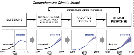
Figure 10.1. Several steps from emissions to climate response contribute to the overall uncertainty of a climate model projection. These uncertainties can be quantified through a combined effort of observation, process understanding, a hierarchy of climate models, and ensemble simulations. In a comprehensive climate model, physical and chemical representations of processes permit a consistent quantification of uncertainty. Note that the uncertainty associated with the future emission path is of an entirely different nature and not addressed in Chapter 10 .Bottom row adapted from Figure 10.26, A1B scenario, for illustration only.
Many of the figures in Chapter 10 are based on the mean and spread of the multi-model ensemble of comprehensive AOGCMs. The reason to focus on the multi-model mean is that averages across structurally different models empirically show better large-scale agreement with observations, because individual model biases tend to cancel (see Chapter8 ). The expanded use of multi-model ensembles of projections of future climate change therefore provides higher quality and more quantitative climate change information compared to the TAR. Even though the ability to simulate present-day mean climate and variability, as well as observed trends, differs across models, no weighting of individual models is applied in calculating the mean. Since the ensemble is strictly an ‘ensemble of opportunity’, without sampling protocol, the spread of models does not necessarily span the full possible range of uncertainty, and a statistical interpretation of the model spread is therefore problematic. However, attempts are made to quantify uncertainty throughout the chapter based on various other lines of evidence, including perturbed physics ensembles specifically designed to study uncertainty within one model framework, and Bayesian methods using observational constraints.
In addition to this coordinated international multi-model experiment, a number of entirely new types of experiments have been performed since the TAR to quantify uncertainty regarding climate model response to external forcings. The extent to which uncertainties in parametrizations translate into the uncertainty in climate change projections is addressed in much greater detail. New calculations of future climate change from the larger suite of SRES scenarios with simple models and Earth System Models of Intermediate Complexity (EMICs) provide additional information regarding uncertainty related to the choice of scenario. Such models also provide estimates of long-term evolution of global mean temperature, ocean heat uptake and sea level rise due to thermal expansion beyond the 21st century, and thus allow climate change commitments to be better constrained.
Climate sensitivity has always been a focus in the IPCC assessments, and this chapter assesses more quantitative estimates of equilibrium climate sensitivity and transient climate response (TCR) in terms of not only ranges but also probabilities within these ranges. Some of these probabilities are now derived from ensemble simulations subject to various observational constraints, and no longer rely solely on expert judgement. This permits a much more complete assessment of model response uncertainties from these sources than ever before. These are now standard benchmark calculations with the global coupled climate models, and are useful to assess model response in the subsequent time-evolving climate change scenario experiments.
With regard to these time-evolving experiments simulating 21st-century climate, since the TAR increased computing capabilities now allow routine performance of multi-member ensembles in climate change scenario experiments with global coupled climate models. This provides the capability to analyse more multi-model results and multi-member ensembles, and yields more probabilistic estimates of time-evolving climate change in the 21st century.
Finally, while future changes in some weather and climate extremes (e.g., heat waves) were addressed in the TAR, there were relatively few studies on this topic available for assessment at that time. Since then, more analyses have been performed regarding possible future changes in a variety of extremes. It is now possible to assess, for the first time, multi-model ensemble results for certain types of extreme events (e.g., heat waves, frost days, etc.). These new studies provide a more complete range of results for assessment regarding possible future changes in these important phenomena with their notable impacts on human societies and ecosystems. A synthesis of results from studies of extremes from observations and model is provided in Chapter 11 .
The use of multi-model ensembles has been shown in other modelling applications to produce simulated climate features that are improved over single models alone (see discussion in Chapters 8 and 9 ). In addition, a hierarchy of models ranging from simple to intermediate to complex allows better quantification of the consequences of various parametrizations and formulations. Very large ensembles (order hundreds) with single models provide the means to quantify parametrization uncertainty. Finally, observed climate characteristics are now being used to better constrain future climate model projections.
10.2 Projected Changes in Emissions, Concentrations and Radiative Forcing
The global projections discussed in this chapter are extensions of the simulations of the observational record discussed in Chapter9 .The simulations of the 19th and 20th centuries are based upon changes in long-lived greenhouse gases (LLGHGs) that are reasonably constrained by the observational record. Therefore, the models have qualitatively similar temporal evolutions of their radiative forcing time histories for LLGHGs (e.g., see Figure 2.23 ). However, estimates of future concentrations of LLGHGs and other radiatively active species are clearly subject to significant uncertainties. The evolution of these species is governed by a variety of factors that are difficult to predict, including changes in population, energy use, energy sources and emissions. For these reasons, a range of projections of future climate change has been conducted using coupled AOGCMs. The future concentrations of LLGHGs and the anthropogenic emissions of sulphur dioxide (SO2), a chemical precursor of sulphate aerosol, are obtained from several scenarios considered representative of low, medium and high emission trajectories. These basic scenarios and other forcing agents incorporated in the AOGCM projections, including several types of natural and anthropogenic aerosols, are discussed in Section 10.2.1 .Developments in projecting radiatively active species and radiative forcing for the early 21st century are considered in Section 10.2.2 .
10.2.1 Emissions Scenarios and Radiative Forcing in the Multi-Model Climate Projections
The temporal evolution of the LLGHGs, aerosols and other forcing agents are described in Sections 10.2.1.1 and 10.2.1.2 .Typically, the future projections are based upon initial conditions extracted from the end of the simulations of the 20th century. Therefore, the radiative forcing at the beginning of the model projections should be approximately equal to the radiative forcing for present-day concentrations relative to pre-industrial conditions. The relationship between the modelled radiative forcing for the year 2000 and the estimates derived in Chapter2 is evaluated in Section 10.2.1.3 .Estimates of the radiative forcing in the multi-model integrations for one of the standard scenarios are also presented in this section. Possible explanations for the range of radiative forcings projected for 2100 are discussed in Section 10.2.1.4 ,including evidence for systematic errors in the formulations of radiative transfer used in AOGCMs. Possible implications of these findings for the range of global temperature change and other climate responses are summarised in Section 10.2.1.5 .
10.2.1.1 The Special Report on Emission Scenarios and Constant-Concentration Commitment Scenarios
The future projections discussed in this chapter are based upon the standard A2, A1B and B2 SRES scenarios ( Nakićenović and Swart, 2000 [NPR] ). The emissions of CO2,methane (CH4)and SO2,the concentrations of CO2,CH4 and nitrous oxide (N2O) and the total radiative forcing for the SRES scenarios are illustrated in Figure 10.26 and summarised for the A1B scenario in Figure 10.1 .The models have been integrated to year 2100 using the projected concentrations of LLGHGs and emissions of SO2 specified by the A1B, B1 and A2 emissions scenarios. Some of the AOGCMs do not include sulphur chemistry, and the simulations from these models are based upon concentrations of sulphate aerosols from Boucher and Pham 2002 [JoC, MoS, ARC] ; see Section 10.2.1.2 ). The simulations for the three scenarios were continued for another 100 to 200 years with all anthropogenic forcing agents held fixed at values applicable to the year 2100 . There is also a new constant-concentration commitment scenario that assumes concentrations are held fixed at year 2000 levels( Section 10.7.1 ). In this idealised scenario, models are initialised from the end of the simulations for the 20th century, the concentrations of radiatively active species are held constant at year 2000 values from these simulations, and the models are integrated to 2100 .
For comparison with this constant composition case, it is useful to note that constant emissions would lead to much larger radiative forcing. For example, constant CO2 emissions at year 2000 values would lead to concentrations reaching about 520 ppm by 2100, close to the B1 case ( Friedlingstein and Solomon, 2005 [PoC, JoC, SRC] ; Hare and Munschausen, 2006; see also FAQ 10.3 ).
10.2.1.2 Forcing by Additional Species and Mechanisms
The forcing agents applied to each AOGCM used to make climate projections are summarised in Table 10.1 .The radiatively active species specified by the SRES scenarios are CO2,CH4,N2O, chlorofluorocarbons (CFCs) and SO2,which is listed in its aerosol form as sulphate (SO4)in the table. The inclusion, magnitude and temporal evolution of the remaining forcing agents listed in Table 10.1 were left to the discretion of the individual modelling groups. These agents include tropospheric and stratospheric ozone, all of the non-sulphate aerosols, the indirect effects of aerosols on cloud albedo and lifetime, the effects of land use and solar variability.
The scope of the treatments of aerosol effects in AOGCMs has increased markedly since the TAR. Seven of the AOGCMs include the first indirect effects and five include the second indirect effects of aerosols on cloud properties( Section 2.4.5 ). Under the more emissions-intensive scenarios considered in this chapter, the magnitude of the first indirect (Twomey) effect can saturate. Johns et al. 2003 [JoC, MoS] ) parametrize the first indirect effect of anthropogenic sulphur (S) emissions as perturbations to the effective radii of cloud drops in simulations of the B1, B2, A2 and A1FI scenarios using UKMO-HadCM3. At 2100, the first indirect forcing ranges from –0.50 to –0.79 Wm–2.The normalised indirect forcing (the ratio of the forcing (Wm–2)to the mass burden of a species (mgm–2), leaving units of W mg–1)decreases by a factor of four, from approximately –7 W mgS–1 in 1860 to between –1 and –2 W mgS–1 by the year 2100 Boucher and Pham 2002 [JoC, MoS, ARC] and Pham et al. 2005 [JoC, MoS, ARC] ) find a comparable projected decrease in forcing efficiency of the indirect effect, from –9.6 W mgS–1 in 1860 to between –2.1 and –4.4 W mgS–1 in 2100 Johns et al. 2003 [JoC, MoS] and Pham et al. 2005 [JoC, MoS, ARC] ) attribute the projected decline to the decreased sensitivity of clouds to greater sulphate concentrations at sufficiently large aerosol burdens.
10.2.1.3 Comparison of Modelled Forcings to Estimates in Chapter2
The forcings used to generate climate projections for the standard SRES scenarios are not necessarily uniform across the multi-model ensemble. Differences among models may be caused by different projections for radiatively active species (see Section 10.2.1.2 )and by differences in the formulation of radiative transfer (see Section 10.2.1.4 ). The AOGCMs in the ensemble include many species that are not specified or constrained by the SRES scenarios, including ozone, tropospheric non-sulphate aerosols, and stratospheric volcanic aerosols. Other types of forcing that vary across the ensemble include solar variability, the indirect effects of aerosols on clouds and the effects of land use change on land surface albedo and other land surface properties( Table 10.1 ). While the time series of LLGHGs for the future scenarios are mostly identical across the ensemble, the concentrations of these gases in the 19th and early 20th centuries were left to the discretion of individual modelling groups. The differences in radiatively active species and the formulation of radiative transfer affect both the 19th- and 20th-century simulations and the scenario integrations initiated from these historical simulations. The resulting differences in the forcing complicate the separation of forcing and response across the multi-model ensemble. These differences can be quantified by comparing the range of shortwave and longwave forcings across the multi-model ensemble against standard estimates of radiative forcing over the historical record. Shortwave and longwave forcing refer to modifications of the solar and infrared atmospheric radiation fluxes, respectively, that are caused by external changes to the climate system( Section 2.2 ).
Table 10.1. Radiative forcing agents in the multi-model global climate projections. See Table 8.1 for descriptions of the models. Entries mean Y: forcing agent is included; C: forcing agent varies with time during the 20th Century Climate in Coupled Models (20C3M) simulations and is set to constant or annually cyclic distribution for scenario integrations; E: forcing agent represented using equivalent CO2;and n.a.: forcing agent is not specified in either the 20th-century or scenario integrations. Numeric codes indicate that the forcing agent is included using data described at 1: http://www.cnrm.meteo.fr/ensembles/public/results/results.html; 2: Boucher and Pham 2002 [JoC, MoS, ARC] ); 3: Yukimoto et al. 2006 [MoS, SRC] ); 4: Meehl, et al., 2006b [JoC, MoS, SRC] ; 5: http://aom.giss.nasa.gov/IN/GHGA1B.LP; and 6: http://sres.ciesin.org/final_data.html.
| Model | Forcing Agents | |||||||||||||||||
|---|---|---|---|---|---|---|---|---|---|---|---|---|---|---|---|---|---|---|
| Greenhouse Gases | Aerosols | Other | ||||||||||||||||
| CO2 | CH4 | N2O | Stratospheric Ozone | Tropospheric Ozone | CFCs | SO4 | Urban | Black carbon | Organic carbon | Nitrate | 1st Indirect | 2nd Indirect | Dust | Volcanic | Sea Salt | Land Use | Solar | |
| BCC-CM1 | Y | Y | Y | Y | C | 4 | 4 | n.a. | n.a. | n.a. | n.a. | n.a. | n.a. | n.a. | C | n.a. | C | C |
| BCCR-BCM2.0 | 1 | 1 | 1 | C | C | 1 | 2 | C | n.a. | n.a. | n.a. | n.a. | n.a. | C | n.a. | C | C | C |
| CCSM3 | 4 | 4 | 4 | 4 | 4 | 4 | 4 | n.a. | 4 | 4 | n.a. | n.a. | n.a. | Y | C | Y | n.a. | C |
| CGCM3.1(T47) | Y | Y | Y | C | C | Y | 2 | n.a. | n.a. | n.a. | n.a. | n.a. | n.a. | C | C | C | C | C |
| CGCM3.1(T63) | Y | Y | Y | C | C | Y | 2 | n.a. | n.a. | n.a. | n.a. | n.a. | n.a. | C | C | C | C | C |
| CNRM-CM3 | 1 | 1 | 1 | Y | Y | 1 | 2 | C | n.a. | n.a. | n.a. | n.a. | n.a. | C | n.a. | C | n.a. | n.a. |
| CSIRO-MK3.0 | Y | E | E | Y | Y | E | Y | n.a. | n.a. | n.a. | n.a. | n.a. | n.a. | n.a. | n.a. | n.a. | n.a. | n.a. |
| ECHAM5/MPI-OM | 1 | 1 | 1 | Y | C | 1 | 2 | n.a. | n.a. | n.a. | n.a. | Y | n.a. | n.a. | n.a. | n.a. | n.a. | n.a. |
| ECHO-G | 1 | 1 | 1 | C | Y | 1 | 6 | n.a. | n.a. | n.a. | n.a. | Y | n.a. | n.a. | C | n.a. | n.a. | C |
| FGOALS-g1.0 | 4 | 4 | 4 | C | C | 4 | 4 | n.a. | n.a. | n.a. | n.a. | n.a. | n.a. | n.a. | n.a. | n.a. | n.a. | C |
| GFDL-CM2.0 | Y | Y | Y | Y | Y | Y | Y | n.a. | Y | Y | n.a. | n.a. | n.a. | C | C | C | C | C |
| GFDL-CM2.1 | Y | Y | Y | Y | Y | Y | Y | n.a. | Y | Y | n.a. | n.a. | n.a. | C | C | C | C | C |
| GISS-AOM | 5 | 5 | 5 | C | C | 5 | 2 | n.a. | n.a. | n.a. | n.a. | n.a. | n.a. | n.a. | n.a. | Y | n.a. | n.a. |
| GISS-EH | Y | Y | Y | Y | Y | Y | Y | n.a. | Y | Y | Y | n.a. | Y | C | Y | C | Y | Y |
| GISS-ER | Y | Y | Y | Y | Y | Y | Y | n.a. | Y | Y | Y | n.a. | Y | C | Y | C | Y | Y |
| INM-CM3.0 | 4 | 4 | 4 | C | C | n.a. | 4 | n.a. | n.a. | n.a. | n.a. | n.a. | n.a. | n.a. | C | n.a. | n.a. | C |
| IPSL-CM4 | 1 | 1 | 1 | n.a. | n.a. | 1 | 2 | n.a. | n.a. | n.a. | n.a. | Y | n.a. | n.a. | n.a. | n.a. | n.a. | n.a. |
| MIROC3.2(H) | Y | Y | Y | Y | Y | Y | Y | n.a. | Y | Y | n.a. | Y | Y | Y | C | Y | C | C |
| MIROC3.2(M) | Y | Y | Y | Y | Y | Y | Y | n.a. | Y | Y | n.a. | Y | Y | Y | C | Y | C | C |
| MRI-CGCM2.3.2 | 3 | 3 | 3 | C | C | 3 | 3 | n.a. | n.a. | n.a. | n.a. | n.a. | n.a. | n.a. | C | n.a. | n.a. | C |
| PCM | Y | Y | Y | Y | Y | Y | Y | n.a. | n.a. | n.a. | n.a. | n.a. | n.a. | n.a. | C | n.a. | n.a. | C |
| UKMO-HadCM3 | Y | Y | Y | Y | Y | Y | Y | n.a. | n.a. | n.a. | n.a. | Y | n.a. | n.a. | C | n.a. | n.a. | C |
| UKMO-HadGEM1 | Y | Y | Y | Y | Y | Y | Y | n.a. | Y | Y | n.a. | Y | Y | n.a. | C | Y | Y | C |
The longwave radiative forcings for the SRES A1B scenario from climate model simulations are compared against estimates using the TAR formulae (see Chapter2 )in Figure 10.2 a. The graph shows the longwave forcings from the TAR and 20 AOGCMs in the multi-model ensemble from 2000 to 2100 . The forcings from the models are diagnosed from changes in top-of-atmosphere fluxes and the forcing for doubled atmospheric CO2 ( Forster and Taylor, 2006 [JoC, MoS, SRC] ). The TAR and median model estimates of the longwave forcing are in very good agreement over the 21st century, with differences ranging from –0.37 to +0.06 Wm–2.For the year 2000, the global mean values from the TAR and median model differ by only –0.13 Wm–2.However, the 5th to 95th percentile range of the models for the period 2080 to 2099 is approximately 3.1 Wm–2,or approximately 47% of the median longwave forcing for that time period.
The corresponding time series of shortwave forcings for the SRES A1B scenario are plotted in Figure 10.2 b. It is evident that the relative differences among the models and between the models and the TAR estimates are larger for the shortwave band. The TAR value is larger than the median model forcing by 0.2 to 0.3 Wm–2 for individual 20-year segments of the integrations. For the year 2000, the TAR estimate is larger by 0.42 Wm–2.In addition, the range of modelled forcings is sufficiently large that it includes positive and negative values for every 20-year period. For the year 2100, the shortwave forcing from individual AOGCMs ranges from approximately –1.7 Wm–2 to +0.4 Wm–2 (5th to 95th percentile). The reasons for this large range include the variety of the aerosol treatments and parametrizations for the indirect effects of aerosols in the multi-model ensemble.
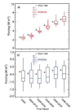
Figure 10.2. Radiative forcings for the period 2000 to 2100 for the SRES A1B scenario diagnosed from AOGCMs and from the TAR ( IPCC, 2001 [NPR] ) forcing formulas ( Forster and Taylor, 2006 [JoC, MoS, SRC] ). (a) Longwave forcing; (b) shortwave forcing. The AOGCM results are plotted with box-and-whisker diagrams representing percentiles of forcings computed from 20 models in the AR4 multi-model ensemble. The central line within each box represents the median value of the model ensemble. The top and bottom of each box shows the 75th and 25th percentiles, and the top and bottom of each whisker displays the 95th and 5th percentile values in the ensemble, respectively. The models included are CCSM3, CGCM3.1 (T47 and T63), CNRM-CM3, CSIRO-MK3, ECHAM5/MPI-OM, ECHO-G, FGOALS-g1.0, GFDL-CM2.0, GFDL-CM2.1, GISS-EH, GISS-ER, INM-CM3.0, IPSL-CM4, MIROC3.2 (medium and high resolution), MRI-CGCM2.3.2, PCM1, UKMO-HadCM3 and UKMO-HadGEM1 (see Table 8.1 for model details).
Since the large range in both longwave and shortwave forcings may be caused by a variety of factors, it is useful to determine the range caused just by differences in model formulation for a given (identical) change in radiatively active species. A standard metric is the global mean, annually averaged all-sky forcing at the tropopause for doubled atmospheric CO2.Estimates of this forcing for 15 of the models in the ensemble are given in Table 10.2 .The shortwave forcing is caused by absorption in the near-infrared bands of CO2.The range in the longwave forcing at 200 mb is 0.84 Wm–2,and the coefficient of variation, or ratio of the standard deviation to mean forcing, is 0.09. These results suggest that up to 35% of the range in longwave forcing in the ensemble for the period 2080 to 2099 is due to the spread in forcing estimates for the specified increase in CO2.The findings also imply that it is not appropriate to use a single best value of the forcing from doubled atmospheric CO2 to relate forcing and response (e.g., climate sensitivity) across a multi-model ensemble. The relationships for a given model should be derived using the radiative forcing produced by the radiative parametrizations in that model. Although the shortwave forcing has a coefficient of variation close to one, the range across the ensemble explains less than 17% of the range in shortwave forcing at the end of the 21st-century simulations. This suggests that species and forcing agents other than CO2 cause the large variation among modelled shortwave forcings.
Table 10.2. All-sky radiative forcing for doubled atmospheric CO2.See Table 8.1 for model details.
| ModelSource | Longwave (Wm–2) | Shortwave (Wm–2) |
|---|---|---|
| CGCM 3.1 (T47/T63)a | 3.39 | –0.07 |
| CSIRO-MK3.0b | 3.42 | 0.05 |
| GISS-EH/ERa | 4.21 | –0.15 |
| GFDL-CM2.0/2.1b | 3.62 | –0.12 |
| IPSL-CM4c | 3.50 | –0.02 |
| MIROC 3.2-hiresd | 3.06 | 0.08 |
| MIROC 3.2-medresd | 2.99 | 0.10 |
| ECHAM5/MPI-OMa | 3.98 | 0.03 |
| MRI-CGCM2.3.2b | 3.75 | –0.28 |
| CCSM3a | 4.23 | –0.28 |
| UKMO-HadCM3a | 4.03 | –0.22 |
| UKMO-HadGEM1a | 4.02 | –0.24 |
| Mean ± standard deviatione | 3.80 ± 0.33 | –0.13 ± 0.11 |
10.2.1.4 Results from the Radiative-Transfer Model Intercomparison Project: Implications for Fidelity of Forcing Projections
Differences in radiative forcing across the multi-model ensemble illustrated in Table 10.2 have been quantified in the Radiative-Transfer Model Intercomparison Project (RTMIP, W.D. Collins et al., 2006 [Ambiguous] ). The basis of RTMIP is an evaluation of the forcings computed by 20 AOGCMs using five benchmark line-by-line (LBL) radiative transfer codes. The comparison is focused on the instantaneous clear-sky radiative forcing by the LLGHGs CO2,CH4,N2O, CFC-11, CFC-12 and the increased water vapour expected in warmer climates. The results of this intercomparison are not directly comparable to the estimates of forcing at the tropopause( Chapter2 ), since the latter include the effects of stratospheric adjustment. The effects of adjustment on forcing are approximately –2% for CH4,–4% forN2O, +5% for CFC-11, +8% for CFC-12 and –13% for CO2 ( IPCC, 1995 [NPR, MoS] ; Hansen et al., 1997 [JoC, MoS, SRC] ). The total (longwave plus shortwave) radiative forcings at 200 mb, a surrogate for the tropopause, are shown in Table 10.3 for climatological mid-latitude summer conditions.
Total forcings calculated from the AOGCM and LBL codes due to the increase in LLGHGs from 1860 to 2000 differ by less than 0.04, 0.49 and 0.10 Wm–2 at the top of model, surface and pseudo-tropopause at 200mb, respectively( Table 10.3 ). Based upon the Student t-test, none of the differences in mean forcings shown in Table 10.3 is statistically significant at the 0.01 level. This indicates that the ensemble mean forcings are in reasonable agreement with the LBL codes. However, the forcings from individual models, for example from doubled atmospheric CO2,span a range at least 10 times larger than that exhibited by the LBL models.
The forcings from doubling atmospheric CO2 from its concentration at 1860 AD are shown in Figure 10.3 aat the top of the model (TOM), 200 hPa( Table 10.3 ), and the surface. The AOGCMs tend to underestimate the longwave forcing at these three levels. The relative differences in the mean forcings are less than 8% for the pseudo-tropopause at 200 hPa but increase to approximately 13% at the TOM and to 33% at the surface. In general, the mean shortwave forcings from the LBL and AOGCM codes are in good agreement at all three surfaces. However, the range in shortwave forcing at the surface from individual AOGCMs is quite large. The coefficient of variation (the ratio of the standard deviation to the mean) for the surface shortwave forcing from AOGCMs is 0.95. In response to a doubling in atmospheric CO2,the specific humidity increases by approximately 20% through much of the troposphere. The changes in shortwave and longwave fluxes due to a 20% increase in water vapour are illustrated in Figure 10.3 b. The mean longwave forcing from increasing water vapour is quite well simulated with the AOGCM codes. In the shortwave, the only significant difference between the AOGCM and LBL calculations occurs at the surface, where the AOGCMs tend to underestimate the magnitude of the reduction in insolation. In general, the biases in the AOGCM forcings are largest at the surface level.
Table 10.3. Total instantaneous forcing at 200 hPa (Wm–2)from AOGCMs and LBL codes in RTMIP (W.D. Collins et al., 2006 [Ambiguous] ). Calculations are for cloud-free climatological mid-latitude summer conditions.
| Radiative Species | CO2 | CO2 | N2O+ CFCs | CH4 + CFCs | All LLGHGs | Water Vapour |
|---|---|---|---|---|---|---|
| Forcinga | 2000–1860 | 2x–1x | 2000–1860 | 2000–1860 | 2000–1860 | 1.2x–1x |
| AOGCM mean | 1.56 | 4.28 | 0.47 | 0.95 | 2.68 | 4.82 |
| AOGCM std. dev. | 0.23 | 0.66 | 0.15 | 0.30 | 0.30 | 0.34 |
| LBL mean | 1.69 | 4.75 | 0.38 | 0.73 | 2.58 | 5.08 |
| LBL std. dev. | 0.02 | 0.04 | 0.12 | 0.12 | 0.11 | 0.16 |
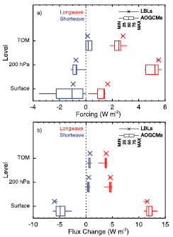
Figure 10.3. Comparison of shortwave and longwave instantaneous radiative forcings and flux changes computed from AOGCMs and line-by-line (LBL) radiative transfer codes (W.D. Collins et al., 2006 [Ambiguous] ). (a) Instantaneous forcing from doubling atmospheric CO2 from its concentration in 1860; b) changes in radiative fluxes caused by the 20% increase in water vapour expected in the climate produced from doubling atmospheric CO2.The forcings and flux changes are computed for clear-sky conditions in mid-latitude summer and do not include effects of stratospheric adjustment. No other well-mixed greenhouse gases are included. The minimum-to-maximum range and median are plotted for five representative LBL codes. The AOGCM results are plotted with box-and-whisker diagrams (see caption for Figure 10.2) representing percentiles of forcings from 20 models in the AR4 multi-model ensemble. The AOGCMs included are BCCRBCM2.0, CCSM3, CGCM3.1(T47 and T63), CNRMCM3, ECHAM5/MPIOM, ECHOG, FGOALSg1.0, GFDLCM2.0, GFDLCM2.1, GISSEH, GISSER, INMCM3.0, IPSLCM4, MIROC3.2 (medium and high resolution), MRICGCM2.3.2, PCM, UKMOHadCM3, and UKMOHadGEM1 (see Table 8.1 for model details). The LBL codes are the Geophysical Fluid Dynamics Laboratory (GFDL) LBL, the Goddard Institute for Space Studies (GISS) LBL3, the National Center for Atmospheric Research (NCAR)/Imperial College of Science, Technology and Medicine (ICSTM) general LBL GENLN2, the National Aeronautics and Space Administration (NASA) Langley Research Center MRTA and the University of Reading Reference Forward Model (RFM).
10.2.1.5 Implications for Range in Climate Response
The results from RTMIP imply that the spread in climate response discussed in this chapter is due in part to the diverse representations of radiative transfer among the members of the multi-model ensemble. Even if the concentrations of LLGHGs were identical across the ensemble, differences in radiative transfer parametrizations among the ensemble members would lead to different estimates of radiative forcing by these species. Many of the climate responses (e.g., global mean temperature) scale linearly with the radiative forcing to first approximation. Therefore, systematic errors in the calculations of radiative forcing should produce a corresponding range in climate responses. Assuming that the RTMIP results( Table 10.3 )are globally applicable, the range of forcings for 1860 to 2000 in the AOGCMs should introduce a ±18% relative range (the 5 to 95% confidence interval) for 2000 in the responses that scale with forcing. The corresponding relative range for doubled atmospheric CO2,which is comparable to the change in CO2 in the B1 scenario by 2100, is ± 25%.
Some recent studies have suggested that the global atmospheric burden of soil dust aerosols could decrease by between 20 and 60% due to reductions in desert areas associated with climate change ( Mahowald and Luo, 2003 [JoC, MoS] Tegen et al. 2004a [JoC, MoS] ,b) compared simulations by the European Centre for Medium Range Weather Forecasts/Max Planck Institute for Meteorology Atmospheric GCM (ECHAM4) and UKMO-HadCM3 that included the effects of climate-induced changes in atmospheric conditions and vegetation cover and the effects of increased CO2 concentrations on vegetation density. These simulations are forced with identical (IS92a) time series for LLGHGs. Their findings suggest that future projections of changes in dust loading are quite model dependent, since the net changes in global atmospheric dust loading produced by the two models have opposite signs. They also conclude that dust from agriculturally disturbed soils is less than 10% of the current burden, and that climate-induced changes in dust concentrations would dominate land use changes under both minimum and maximum estimates of increased agricultural area by 2050 .
10.2.2 Recent Developments in Projections of Radiative Species and Forcing for the 21st Century
Estimation of ozone forcing for the 21st century is complicated by the short chemical lifetime of ozone compared to atmospheric transport time scales and by the sensitivity of the radiative forcing to the vertical distribution of ozone. Gauss et al. 2003 [JoC, MoS] ) calculate the forcing by anthropogenic increases of tropospheric ozone through 2100 from 11 different chemical transport models integrated with the SRES A2p scenario. The A2p scenario is the preliminary version of the marker A2 scenario and has nearly identical time series of LLGHGs and forcing. Since the emissions of CH4,carbon monoxide (CO), reactive nitrogen oxides (NOx)and volatile organic compounds (VOCs), which strongly affect the formation of ozone, are maximised in the A2p scenario, the modelled forcings should represent an upper bound for the forcing produced under more constrained emissions scenarios. The 11 models simulate an increase in tropospheric ozone of 11.4 to 20.5 Dobson units (DU) by 2100, corresponding to a range of radiative forcing from 0.40 to 0.78 Wm–2.Under this scenario, stratospheric ozone increases by between 7.5 and 9.3 DU, which raises the radiative forcing by an additional 0.15 to 0.17 Wm–2.
One aspect of future direct aerosol radiative forcing omitted from all but 2 (the GISS-EH and GISS-ER models) of the 23 AOGCMS analysed in AR4 (see Table 8.1 for list) is the role of nitrate aerosols. Rapid increases in NOx emissions could produce enough nitrate aerosol to offset the expected decline in sulphate forcing by 2100 Adams et al. 2001 [JoC, MoS] ) compute the radiative forcing by sulphate and nitrate accounting for the interactions among sulphate, nitrate and ammonia. For 2000, the sulphate and nitrate forcing are –0.95 and –0.19 Wm–2,respectively. Under the SRES A2 scenario, by 2100 declining SO2 emissions cause the sulphate forcing to drop to –0.85 Wm–2,while the nitrate forcing rises to –1.28 Wm–2.Hence, the total sulphate-nitrate forcing increases in magnitude from –1.14 Wm–2 to –2.13 Wm–2 rather than declining as models that omit nitrates would suggest. This projection is consistent with the large increase in coal burning forecast as part of the A2 scenario.
Recent field programs focused on Asian aerosols have demonstrated the importance of black carbon (BC) and organic carbon (OC) for regional climate, including potentially significant perturbations of the surface energy budget and hydrological cycle ( Ramanathan et al., 2001 [JoC, ARC] ). Modelling groups have developed a multiplicity of projections for the concentrations of these aerosol species. For example, Takemura et al. 2001 [MoS, ARC] ) use data sets for BC released by fossil fuel and biomass burning ( Cooke and Wilson, 1996 [JoC, MoS] ) under current conditions and scale them by the ratio of future to present-day CO2.The emissions of OC are derived using OC:BC ratios estimated for each source and fuel type. Koch 2001 [JoC, MoS] ) models the future radiative forcing of BC by scaling a different set of present-day emission inventories by the ratio of future to present-day CO2 emissions. There are still large uncertainties associated with current inventories of BC and OC ( Bond et al., 2004 [JoC] ), the ad hoc scaling methods used to produce future emissions, and considerable variation among estimates of the optical properties of carbonaceous aerosols ( Kinne et al., 2006 [MoS, ARC] ). Given these uncertainties, future projections of forcing by BC and OC should be quite model dependent.
Recent evidence suggests that there are detectable anthropogenic increases in stratospheric sulphate (e.g., Myhre et al., 2004 [JoC, ARC] ), water vapour (e.g., Forster and Shine, 2002 [JoC] ), and condensed water in the form of aircraft contrails. However, recent modelling studies suggest that these forcings are relatively minor compared to the major LLGHGs and aerosol species. Marquart et al. 2003 [JoC, MoS, ARC] ) estimate that the radiative forcing by contrails will increase from 0.035 Wm–2 in 1992 to 0.094 Wm–2 in 2015 and to 0.148 Wm–2 in 2050 . The rise in forcing is due to an increase in subsonic aircraft traffic following estimates of future fuel consumption ( Penner et al., 1999 [NPR, ARC] ). These estimates are still subject to considerable uncertainties related to poor constraints on the microphysical properties, optical depths and diurnal cycle of contrails ( Myhre and Stordal, 2001 [JoC, ARC] , 2002; Marquart et al., 2003 [JoC, MoS, ARC] Pitari et al. 2002 [JoC, MoS] ) examine the effect of future emissions under the A2 scenario on stratospheric concentrations of sulphate aerosol and ozone. By 2030, the mass of stratospheric sulphate increases by approximately 33%, with the majority of the increase contributed by enhanced upward fluxes of anthropogenic SO2 through the tropopause. The increase in direct shortwave forcing by stratospheric aerosols in the A2 scenario during 2000 to 2030 is –0.06 Wm–2.
10.3 Projected Changes in the Physical Climate System
The context for the climate change results presented here is set in Chapter8 (evaluation of simulation skill of the control runs and inherent natural variability of the global coupled climate models), and in Chapter9 (evaluation of the simulations of 20th-century climate using the global coupled climate models). Table 8.1 describes the characteristics of the models, and Table 10.4 summarises the climate change experiments that have been performed with the AOGCMs and other models that are assessed in this chapter.
The TAR showed multi-model results for future changes in climate from simple 1% yr–1 CO2 increase experiments, and from several scenarios including the older IS92a, and, new to the TAR, two SRES scenarios (A2 and B2). For the latter, results from nine models were shown for globally averaged temperature change and regional changes. As noted in Section 10.1 ,since the TAR, an unprecedented internationally coordinated climate change experiment has been performed by 23 models from around the world, listed in Table 10.4 along with the results submitted. This larger number of models running the same experiments allows better quantification of the multi-model signal as well as uncertainty regarding spread across the models (in this section), and also points the way to probabilistic estimates of future climate change( Section 10.5 ). The emission scenarios considered here include one of the SRES scenarios from the TAR, scenario A2, along with two additional scenarios, A1B and B1 (see Section 10.2 for details regarding the scenarios). This is a subset of the SRES marker scenarios used in the TAR, and they represent ‘low’ (B1), ‘medium’ (A1B) and ‘high’ (A2) scenarios with respect to the prescribed concentrations and the resulting radiative forcing, relative to the SRES range. This choice was made solely due to the limited computational resources for multi-model simulations using comprehensive AOGCMs and does not imply any preference or qualification of these three scenarios over the others. Qualitative conclusions derived from those three scenarios are in most cases also valid for other SRES scenarios.
Additionally, three climate change commitment experiments were performed, one where concentrations of greenhouse gases were held fixed at year 2000 values (constant composition commitment) and the models were run to 2100 (termed 20th-century stabilisation here), and two where concentrations were held fixed at year 2100 values for A1B and B1, and the models were run for an additional 100 to 200 years (see Section 10.7 ). The span of the experiments is shown in Figure 10.4 .

*Some of the ensemble members using the CCSM3 were run on the Earth Simulator in Japan in collaboration with the Central Research Institute of Electric Power Industry (CRIEPI).
Table 10.4. Summary of climate change model experiments produced with AOGCMs. Numbers in each scenario column indicate how many ensemble members were produced for each model. Coloured fields indicate that some but not necessarily all variables of the specific data type (separated by climate system component and time interval) were available for download at the PCMDI to be used in this report; ISCCP is the International Satellite Cloud Climatology Project. Additional data has been submitted for some models and may subsequently become available. Where different colour shadings are given in the legend, the colour indicates whether data from a single or from multiple ensemble members is available. Details on the scenarios, variables and models can be found at the PCMDI webpage (http://www-pcmdi.llnl.gov/ipcc/about_ipcc.php). Model IDs are the same as in Table 8.1, which provides details of the models.
This section considers the basic changes in climate over the next hundred years simulated by current climate models under non-mitigation anthropogenic forcing scenarios. While we assess all studies in this field, the focus is on results derived by the authors from the new data set for the three SRES scenarios. Following the TAR, means across the multi-model ensemble are used to illustrate representative changes. Means are able to simulate the contemporary climate more accurately than individual models, due to biases tending to compensate each other ( Phillips and Gleckler, 2006 [MoS, SRC] ). It is anticipated that this holds for changes in climate also( Chapter9 ). The mean temperature trends from the 20th-century simulations are included in Figure 10.4 .While the range of model results is indicated here, the consideration of uncertainty resulting from this range is addressed more completely in Section 10.5 .The use of means has the additional advantage of reducing the ‘noise’ associated with internal or unforced variability in the simulations. Models are equally weighted here, but other options are noted in Section 10.5 .Lists of the models used in the results are provided in the Supplementary Material for this Chapter.
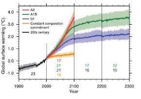
Figure 10.4. Multi-model means of surface warming (relative to 1980 – 1999 ) for the scenarios A2, A1B and B1, shown as continuations of the 20th-century simulation. Values beyond 2100 are for the stabilisation scenarios (see Section 10.7 ). Linear trends from the corresponding control runs have been removed from these time series. Lines show the multi-model means, shading denotes the ±1 standard deviation range of individual model annual means. Discontinuities between different periods have no physical meaning and are caused by the fact that the number of models that have run a given scenario is different for each period and scenario, as indicated by the coloured numbers given for each period and scenario at the bottom of the panel. For the same reason, uncertainty across scenarios should not be interpreted from this figure (see Section 10.5.4.6 for uncertainty estimates).
Standard metrics for response of global coupled models are the equilibrium climate sensitivity, defined as the equilibrium globally averaged surface air temperature change for a doubling of CO2 for the atmosphere coupled to a non-dynamic slab ocean, and the TCR, defined as the globally averaged surface air temperature change at the time of CO2 doubling in the 1% yr–1 transient CO2 increase experiment. The TAR showed results for these 1% simulations, and Section 10.5.2 discusses equilibrium climate sensitivity, TCR and other aspects of response. Chapter8 includes processes and feedbacks involved with these metrics.
10.3.1 Time-Evolving Global Change
The globally averaged surface warming time series from each model in the MMD is shown in Figure 10.5 ,either as a single member (if that was all that was available) or a multi-member ensemble mean, for each scenario in turn. The multi-model ensemble mean warming is also plotted for each case. The surface air temperature is used, averaged over each year, shown as an anomaly relative to the 1980 to 1999 period and offset by any drift in the corresponding control runs in order to extract the forced response. The base period was chosen to match the contemporary climate simulation that is the focus of previous chapters. Similar results have been shown in studies of these models (e.g., Xu et al., 2005 [MoS, SRC] ; Meehl et al., 2006b [JoC, MoS, SRC] ; Yukimoto et al., 2006 [MoS, SRC] ). Interannual variability is evident in each single-model series, but little remains in the ensemble mean because most of this is unforced and is a result of internal variability, as was presented in detail in Section 9.2.2 of TAR. Clearly, there is a range of model results for each year, but over time this range due to internal variability becomes smaller as a fraction of the mean warming. The range is somewhat smaller than the range of warming at the end of the 21st century for the A2 scenario in the comparable Figure 9.6 of the TAR, despite the larger number of models here (the ensemble mean warming is comparable, +3.0°C in the TAR for 2071 to 2100 relative to 1961 to 1990, and +3.13°C here for 2080 to 2099 relative to 1980 to 1999, Table 10.5 ). Consistent with the range of forcing presented in Section 10.2 ,the warming by 2100 is largest in the high greenhouse gas growth scenario A2, intermediate in the moderate growth A1B, and lowest in the low growth B1. Naturally, models with high sensitivity tend to simulate above-average warming in each scenario. The trends of the multi-model mean temperature vary somewhat over the century because of the varying forcings, including that of aerosols (see Section 10.2 ). This is illustrated in Figure 10.4 ,which shows the mean for A1B exceeding that for A2 around 2040 . The time series beyond 2100 are derived from the extensions of the simulations (those available) under the idealised constant composition commitment experiments( Section 10.7.1 ).
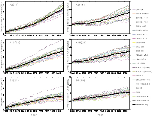
Figure 10.5. Time series of globally averaged (left) surface warming (surface air temperature change, °C) and (right) precipitation change (%) from the various global coupled models for the scenarios A2 (top), A1B (middle) and B1 (bottom). Numbers in parentheses following the scenario name represent the number of simulations shown. Values are annual means, relative to the 1980 to 1999 average from the corresponding 20th-century simulations, with any linear trends in the corresponding control run simulations removed. A three-point smoothing was applied. Multi-model (ensemble) mean series are marked with black dots. See Table 8.1 for model details.
Internal variability in the model response is reduced by averaging over 20-year time periods. This span is shorter than the traditional 30-year climatological period, in recognition of the transient nature of the simulations, and of the larger size of the ensemble. This analysis focuses on three periods over the coming century: an early-century period 2011 to 2030, a mid-century period 2046 to 2065 and the late-century period 2080 to 2099, all relative to the 1980 to 1999 means. The multi-model ensemble mean warmings for the three future periods in the different experiments are given in Table 10.5 ,among other results. The close agreement of warming for the early century, with a range of only 0.05°C among the SRES cases, shows that no matter which of these non-mitigation scenarios is followed, the warming is similar on the time scale of the next decade or two. Note that the precision given here is only relevant for comparison between these means. As evident in Figure 10.4 and discussed in Section 10.5 ,uncertainties in the projections are larger. It is also worth noting that half of the early-century climate change arises from warming that is already committed to under constant composition (0.37°C for the early century). By mid-century, the choice of scenario becomes more important for the magnitude of warming, with a range of 0.46°C, and with about one-third of that warming due to climate change that is already committed to. By the late century, there are clear consequences for which scenario is followed, with a range of 1.3°C in these results, with as little as 18% of that warming coming from climate change that is already committed to.
Table 10.5. Global mean warming (annual mean surface air temperature change) from the multi-model ensemble mean for four time periods relative to 1980 to 1999 for each of the available scenarios. (The mean for the base period is 13.6°C). Also given are two measures of agreement of the geographic scaled patterns of warming (the fields in Figure 10.8 normalised by the global mean), relative to the A1B 2080 to 2099 case. First the non-dimensional M value (see Section 10.3.2.1 )and second (in italics) the global mean absolute error (mae, or difference, in °C/°C) between the fields, both multiplied by 100 for brevity. Here M = (2/π) arcsin[1 – mse / (VX +VY + (GX –GY)2)], with mse the mean square error between the two fields X and Y, and V and G are variance and global mean of the fields (as subscripted). Values of 1 for M and 0 for mae indicate perfect agreement with the standard pattern. ‘Commit’ refers to the constant composition commitment experiment. Note that warming values for the end of the 21st century, given here as the average of years 2080 to 2099, are for a somewhat different averaging period than used in Figure 10.29 ( 2090 – 2099 ); the longer averaging period here is consistent with the comparable averaging period for the geographic plots in this section and is intended to smooth spatial noise.
| Global mean warming (°C) | Measures of agreement (M × 100, mae × 100) | |||||||
|---|---|---|---|---|---|---|---|---|
| 2011–2030 | 2046–2065 | 2080–2099 | 2180–2199 | 2011–2030 | 2046–2065 | 2080–2099 | 2180–2199 | |
| A2 | 0.64 | 1.65 | 3.13 | 83, 8 | 91, 4 | 93, 3 | ||
| A1B | 0.69 | 1.75 | 2.65 | 3.36 | 88, 5 | 94, 4 | 100, 0 | 90, 5 |
| B1 | 0.66 | 1.29 | 1.79 | 2.10 | 86, 6 | 89, 4 | 92, 3 | 86, 6 |
| Commita | 0.37 | 0.47 | 0.56 | 74, 11 | 66, 13 | 68, 13 | ||
Global mean precipitation increases in all scenarios( Figure 10.5 ,right column), indicating an intensification of the hydrological cycle. Douville et al. 2002 [JoC] ) show that this is associated with increased water-holding capacity of the atmosphere in addition to other processes. The multi-model mean varies approximately in proportion to the mean warming, though uncertainties in future hydrological cycle behaviour arise due in part to the different responses of tropical precipitation across models ( Douville et al., 2005 [JoC] ). Expressed as a percentage of the mean simulated change for 1980 to 1999 (2.83 mm day–1), the rate varies from about 1.4% °C–1 in A2 to 2.3% °C–1 in the constant composition commitment experiment (for a table corresponding to Table 10.5 but for precipitation, see the Supplementary Material, Table S10.1). These increases are less than increases in extreme precipitation events, consistent with energetic constraints (see Sections 9.5.4.2 and 10.3.6.1 )
10.3.2 Patterns of Change in the 21st Century
10.3.2.1 Warming
The TAR noted that much of the regional variation of the annual mean warming in the multi-model means is associated with high- to low-latitude contrast. This can be better quantified from the new multi-model mean in terms of zonal averages. A further contrast is provided by partitioning the land and ocean values based on model data interpolated to a standard grid. Figure 10.6 illustrates the late-century A2 case, with all values shown both in absolute terms and relative to the global mean warming. Warming over land is greater than the mean except in the southern mid-latitudes, where the warming over ocean is a minimum. Warming over ocean is smaller than the mean except at high latitudes, where sea ice changes have an influence. This pattern of change illustrated by the ratios is quite similar across the scenarios. The commitment case (shown), discussed in Section 10.7.1 ,has relatively smaller warming of land, except in the far south, which warms closer to the global rate. At nearly all latitudes, the A1B and B1 warming ratios lie between A2 and commitment, with A1B particularly close to the A2 results. Aside from the commitment case, the ratios for the other time periods are also quite similar to those for A2. Regional patterns and precipitation contrasts are discussed in Section 10.3.2.3 .
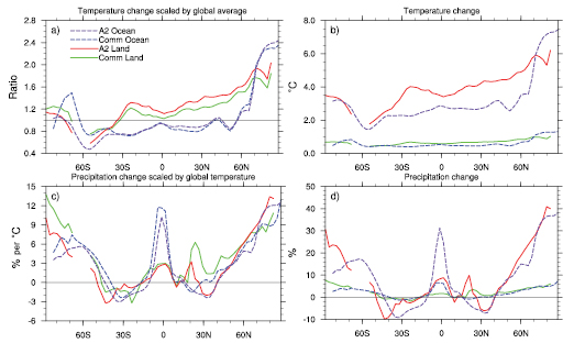
Figure 10.6. Zonal means over land and ocean separately, for annual mean surface warming (a, b) and precipitation (c, d), shown as ratios scaled with the global mean warming (a, c) and not scaled (b, d). Multi-model mean results are shown for two scenarios, A2 and Commitment (see Section 10.7 ), for the period 2080 to 2099 relative to the zonal means for 1980 to 1999 . Results for individual models can be seen in the Supplementary Material for this chapter.
Figure 10.7 shows the zonal mean warming for the A1B scenario at each latitude from the bottom of the ocean to the top of the atmosphere for the three 21st-century periods used in Table 10.5 .To produce this ensemble mean, the model data were first interpolated to standard ocean depths and atmospheric pressures. Consistent with the global transfer of excess heat from the atmosphere to the ocean, and the difference between warming over land and ocean, there is some discontinuity between the plotted means of the lower atmosphere and the upper ocean. The relatively uniform warming of the troposphere and cooling of the stratosphere in this multi-model mean are consistent with the changes shown in Figure 9.8 of the TAR, but now its evolution during the 21st century under this scenario can also be seen. Upper-tropospheric warming reaches a maximum in the tropics and is seen even in the early-century time period. The pattern is very similar over the three periods, consistent with the rapid adjustment of the atmosphere to the forcing. These changes are simulated with good consistency among the models. The larger values of both signs are stippled, indicating that the ensemble mean is larger in magnitude than the inter-model standard deviation. The ratio of mean to standard deviation can be related to formal tests of statistical significance and confidence intervals, if the individual model results were to be considered a sample.
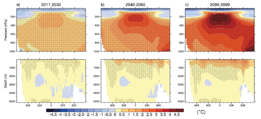
Figure 10.7. Zonal means of change in atmospheric (top) and oceanic (bottom) temperatures (°C), shown as cross sections. Values are the multi-model means for the A1B scenario for three periods (a–c). Stippling denotes regions where the multi-model ensemble mean divided by the multi-model standard deviation exceeds 1.0 (in magnitude). Anomalies are relative to the average of the period 1980 to 1999 . Results for individual models can be seen in the Supplementary Material for this chapter.
The ocean warming evolves more slowly. There is initially little warming below the mixed layer, except at some high latitudes. Even as a ratio with mean surface warming, later in the century the temperature increases more rapidly in the deep ocean, consistent with results from individual models (e.g., Watterson, 2003 [JoC, MoS, SRC] ; Stouffer, 2004 [JoC, SRC] ). This rapid warming of the atmosphere and the slow penetration of the warming into the ocean has implications for the time scales of climate change commitment( Section 10.7 ). It has been noted in a five-member multi-model ensemble analysis that, associated with the changes in temperature of the upper ocean in Figure 10.7 ,the tropical Pacific Ocean heat transport remains nearly constant with increasing greenhouse gases due to the compensation of the subtropical cells and the horizontal gyre variations, even as the subtropical cells change in response to changes in the trade winds ( Hazeleger, 2005 [JoC] ). Additionally, a southward shift of the Antarctic Circumpolar Current is projected to occur in a 15-member multi-model ensemble, due to changes in surface winds in a future warmer climate ( Fyfe and Saenko, 2005 [JoC, ARC] ). This is associated with a poleward shift of the westerlies at the surface (see Section 10.3.6 )and in the upper troposphere particularly notable in the Southern Hemisphere (SH) ( Stone and Fyfe, 2005 [JoC, ARC] ), and increased relative angular momentum from stronger westerlies ( Räisänen, 2003 [JoC, SRC] ) and westerly momentum flux in the lower stratosphere particularly in the tropics and southern mid-latitudes ( Watanabe et al., 2005 [SRC] ). The surface wind changes are associated with corresponding changes in wind stress curl and horizontal mass transport in the ocean ( Saenko et al., 2005 [JoC, ARC] ).
Global-scale patterns for each of the three scenarios and time periods are given in Figure 10.8 .In each case, greater warming over most land areas is evident (e.g., Kunkel and Liang, 2005 [JoC, MoS, ARC] ). Over the ocean, warming is relatively large in the Arctic and along the equator in the eastern Pacific (see Sections 10.3.5.2 and 10.3.5.3 ), with less warming over the North Atlantic and the Southern Ocean (e.g., Xu et al., 2005 [MoS, SRC] ). Enhanced oceanic warming along the equator is also evident in the zonal means of Figure 10.6 ,and can be associated with oceanic heat flux changes ( Watterson, 2003 [JoC, MoS, SRC] ) and forced by the atmosphere ( Liu et al., 2005 [JoC] ).
Fields of temperature change have a similar structure, with the linear correlation coefficient as high as 0.994 between the late-century A2 and A1B cases. As for the zonal means, the fields normalised by the mean warming are very similar. The strict agreement between the A1B field, as a standard, and the others is quantified in Table 10.5 ,by the absolute measure M ( Watterson, 1996 [JoC, MoS, SRC] ; a transformation of a measure of ( Mielke, 1991 ) ), with unity meaning identical fields and zero meaning no similarity (the expected value under random rearrangement of the data on the grid of the measure prior to the arcsin transformation). Values of M become progressively larger later in the 21st century, with values of 0.9 or larger for the late 21st century, thus confirming the closeness of the scaled patterns in the late-century cases. The deviation from unity is approximately proportional to the mean absolute difference. The earlier warming patterns are also similar to the standard case, particularly for the same scenario A1B. Furthermore, the zonal means over land and ocean considered above are representative of much of the small differences in warming ratio. While there is some influence of differences in forcing patterns among the scenarios, and of effects of oceanic uptake and heat transport in modifying the patterns over time, there is also support for the role of atmospheric heat transport in offsetting such influences (e.g., Boer and Yu, 2003b [JoC] ; Watterson and Dix, 2005 [JoC, MoS, SRC] Dufresne et al. 2005 [JoC, SRC] ) show that aerosol contributes a modest cooling of the Northern Hemisphere (NH) up to the mid-21st century in the A2 scenario.
Such similarities in patterns of change have been described by Mitchell 2003 [JoC, MoS] and Harvey 2004 [JoC] ). They aid the efficient presentation of the broad scale multi-model results, as patterns depicted for the standard A1B 2080 to 2099 case are usually typical of other cases. This largely applies to other seasons and also other variables under consideration here. Where there is similarity of normalised changes, values for other cases can be estimated by scaling by the appropriate ratio of global means from Table 10.5 .Note that for some quantities like variability and extremes, such scaling is unlikely to work. The use of such scaled results in combination with global warmings from simple models is discussed in Section 11.10.1 .
As for the zonal means (aside from the Arctic Ocean), consistency in local warmings among the models is high (stippling is omitted in Figure 10.8 for clarity). Only in the central North Atlantic and the far south Pacific in 2011 to 2030 is the mean change less than the standard deviation, in part a result of ocean model limitations there( Section 8.3.2 ). Some regions of high-latitude surface cooling occur in individual models.
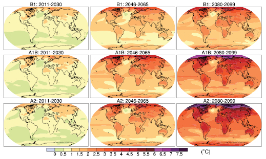
Figure 10.8. Multi-model mean of annual mean surface warming (surface air temperature change, °C) for the scenarios B1 (top), A1B (middle) and A2 (bottom), and three time periods, 2011 to 2030 (left), 2046 to 2065 (middle) and 2080 to 2099 (right). Stippling is omitted for clarity (see text). Anomalies are relative to the average of the period 1980 to 1999 . Results for individual models can be seen in the Supplementary Material for this chapter.
The surface warming fields for the extratropical winter and summer seasons, December to February (DJF) and June to August (JJA), are shown for scenario A1B in Figure 10.9 .The high-latitude warming is rather seasonal, being larger in winter as a result of sea ice and snow, as noted in Chapter 9 of the TAR. However, the relatively small warming in southern South America is more extensive in southern winter. Similar patterns of change in earlier model simulations are described by Giorgi et al. 2001 [JoC, MoS, ARC] ).
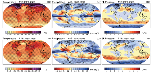
Figure 10.9. Multi-model mean changes in surface air temperature (°C, left), precipitation (mm day–1,middle) and sea level pressure (hPa, right) for boreal winter (DJF, top) and summer (JJA, bottom). Changes are given for the SRES A1B scenario, for the period 2080 to 2099 relative to 1980 to 1999 . Stippling denotes areas where the magnitude of the multi-model ensemble mean exceeds the inter-model standard deviation. Results for individual models can be seen in the Supplementary Material for this chapter.
10.3.2.2 Cloud and Diurnal Cycle
In addition to being an important link to humidity and precipitation, cloud cover plays an important role for the sensitivity of the general circulation models (GCMs; e.g., Soden and Held, 2006 [JoC, MoS, ARC] ) and for the diurnal temperature range (DTR) over land (e.g., Dai and Trenberth, 2004 [PoC, JoC, MoS, ARC] and references therein) so this section considers the projection of these variables now made possible by multi-model ensembles. Cloud radiative feedbacks to greenhouse gas forcing are sensitive to the elevation, latitude and hence temperature of the clouds, in addition to their optical depth and their atmospheric environment (see Section 8.6.3.2 ). Current GCMs simulate clouds through various complex parametrizations (see Section 8.2.1.3 )to produce cloud cover quantified by an area fraction within each grid square and each atmospheric layer. Taking multi-model ensemble zonal means of this quantity interpolated to standard pressure levels and latitudes shows increases in cloud cover at all latitudes in the vicinity of the tropopause, and mostly decreases below, indicating an increase in the altitude of clouds overall( Figure 10.10 a). This shift occurs consistently across models. Outside the tropics the increases aloft are rather consistent, as indicated by the stippling in the figure. Near-surface amounts increase at some latitudes. The mid-level mid-latitude decreases are very consistent, amounting to as much as one-fifth of the average cloud fraction simulated for 1980 to 1999 .
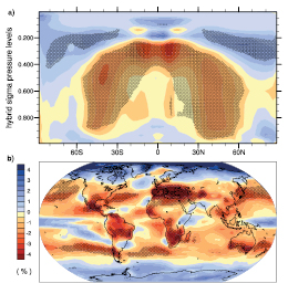
Figure 10.10. Multi-model mean changes in (a) zonal mean cloud fraction (%), shown as a cross section though the atmosphere, and (b) total cloud area fraction (percent cover from all models). Changes are given as annual means for the SRES A1B scenario for the period 2080 to 2099 relative to 1980 to 1999 . Stippling denotes areas where the magnitude of the multi-model ensemble mean exceeds the inter-model standard deviation. Results for individual models can be seen in the Supplementary Material for this chapter.
The total cloud area fraction from an individual model represents the net coverage over all the layers, after allowance for the overlap of clouds, and is an output included in the data set. The change in the ensemble mean of this field is shown in Figure 10.10 b. Much of the low and middle latitudes experience a decrease in cloud cover, simulated with some consistency. There are a few low-latitude regions of increase, as well as substantial increases at high latitudes. The larger changes relate well to changes in precipitation discussed in Section 10.3.2.3 .While clouds need not be precipitating, moderate spatial correlation between cloud cover and precipitation holds for seasonal means of both the present climate and future changes.
The radiative effect of clouds is represented by the cloud radiative forcing diagnostic (see Section 8.6.3.2 ). This can be evaluated from radiative fluxes at the top of the atmosphere calculated with or without the presence of clouds that are output by the GCMs. In the multi-model mean (not shown) values vary in sign over the globe. The global and annual mean averaged over the models, for 1980 to 1999, is –22.3 Wm–2.The change in mean cloud radiative forcing has been shown to have different signs in a limited number of previous modelling studies ( Meehl et al., 2004b [JoC, MoS, SRC] ; Tsushima et al., 2006 [JoC, MoS] ). Figure 10.11 ashows globally averaged cloud radiative forcing changes for 2080 to 2099 under the A1B scenario for individual models of the data set, which have a variety of different magnitudes and even signs. The ensemble mean change is –0.6 Wm–2.This range indicates that cloud feedback is still an uncertain feature of the global coupled models (see Section 8.6.3.2.2 ).
The DTR has been shown to be decreasing in several land areas of the globe in 20th-century observations (see Section 3.2.2.7 ), together with increasing cloud cover (see also Section 9.4.2.3 ). In the multi-model mean of present climate, DTR over land is indeed closely spatially anti-correlated with the total cloud cover field. This is true also of the 21st-century changes in the fields under the A1B scenario, as can be seen by comparing the change in DTR shown in Figure 10.11 bwith the cloud area fraction shown in Figure 10.10 b. Changes in DTR reach a magnitude of 0.5°C in some regions, with some consistency among the models. Smaller widespread decreases are likely due to the radiative effect of the enhanced greenhouse gases including water vapour (see also Stone and Weaver, 2002 [JoC, MoS, SRC] ). Further discussion of DTR is provided in Section 10.3.6.2 .
In addition to the DTR, Kitoh and Arakawa 2005 [JoC, MoS, SRC] ) document changes in the regional patterns of diurnal precipitation over the Indonesian region, and show that over ocean, nighttime precipitation decreases and daytime precipitation increases, while over land the opposite is the case, thus producing a decrease in the diurnal precipitation amplitude over land and ocean. They attribute these changes to a larger nighttime temperature increase over land due to increased greenhouse gases.
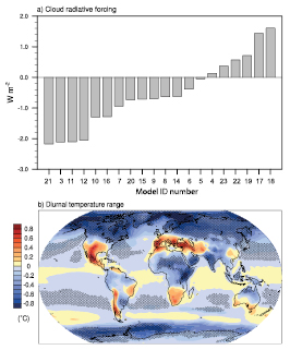
Figure 10.11. Changes in (a) global mean cloud radiative forcing (Wm–2)from individual models (see Table 10.4 for the list of models) and (b) multi-model mean diurnal temperature range (°C). Changes are annual means for the SRES A1B scenario for the period 2080 to 2099 relative to 1980 to 1999 . Stippling denotes areas where the magnitude of the multi-model ensemble mean exceeds the inter-model standard deviation. Results for individual models can be seen in the Supplementary Material for this chapter.
10.3.2.3 Precipitation and Surface Water
Models simulate that global mean precipitation increases with global warming. However, there are substantial spatial and seasonal variations in this field even in the multi-model means depicted in Figure 10.9 .There are fewer areas stippled for precipitation than for the warming, indicating more variation in the magnitude of change among the ensemble of models. Increases in precipitation at high latitudes in both seasons are very consistent across models. The increases in precipitation over the tropical oceans and in some of the monsoon regimes (e.g., South Asian monsoon in JJA, Australian monsoon in DJF) are notable, and while not as consistent locally, considerable agreement is found at the broader scale in the tropics ( Neelin et al., 2006 [JoC, MoS] ). There are widespread decreases in mid-latitude summer precipitation, except for increases in eastern Asia. Decreases in precipitation over many subtropical areas are evident in the multi-model ensemble mean, and consistency in the sign of change among the models is often high ( Wang, 2005 [JoC, MoS] ), particularly in some regions like the tropical Central American-Caribbean ( Neelin et al., 2006 [JoC, MoS] ). Further discussion of regional changes is presented in Chapter 11 .
The global map of the A1B 2080 to 2099 change in annual mean precipitation is shown in Figure 10.12 ,along with other hydrological quantities from the multi-model ensemble. Emori and Brown 2005 [JoC, SRC] ) show percentage changes of annual precipitation from the ensemble. Increases of over 20% occur at most high latitudes, as well as in eastern Africa, central Asia and the equatorial Pacific Ocean. The change over the ocean between 10°S and 10°N accounts for about half the increase in the global mean( Figure 10.5 ). Substantial decreases, reaching 20%, occur in the Mediterranean region ( Rowell and Jones, 2006 [JoC, MoS, ARC] ), the Caribbean region ( Neelin et al., 2006 [JoC, MoS] ) and the subtropical western coasts of each continent. Overall, precipitation over land increases by about 5%, while precipitation over ocean increases 4%, but with regional changes of both signs. The net change over land accounts for 24% of the global mean increase in precipitation, a little less than the areal proportion of land (29%). In Figure 10.12 ,stippling indicates that the sign of the local change is common to at least 80% of the models (with the alternative test shown in the Supplementary Material). This simpler test for consistency is of particular interest for quantities where the magnitudes for the base climate vary across models.
These patterns of change occur in the other scenarios, although with agreement (by the metric M) a little lower than for the warming. The predominance of increases near the equator and at high latitudes, for both land and ocean, is clear from the zonal mean changes of precipitation included in Figure 10.6 .The results for change scaled by global mean warming are rather similar across the four scenarios, an exception being a relatively large increase over the equatorial ocean for the commitment case. As with surface temperature, the A1B and B1 scaled values are always close to the A2 results. The zonal means of the percentage change map (shown in Figure 10.6 )feature substantial decreases in the subtropics and lower mid-latitudes of both hemispheres in the A2 case, even if increases occur over some regions.
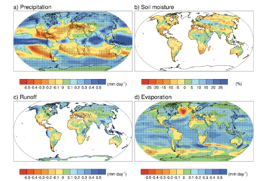
Figure 10.12. Multi-model mean changes in (a) precipitation (mm day–1), (b) soil moisture content (%), (c) runoff (mm day–1)and (d) evaporation (mm day–1). To indicate consistency in the sign of change, regions are stippled where at least 80% of models agree on the sign of the mean change. Changes are annual means for the SRES A1B scenario for the period 2080 to 2099 relative to 1980 to 1999 . Soil moisture and runoff changes are shown at land points with valid data from at least 10 models. Details of the method and results for individual models can be found in the Supplementary Material for this chapter.
Wetherald and Manabe 2002 [JoC, MoS] ) provide a good description of the mechanism of hydrological change simulated by GCMs. In GCMs, the global mean evaporation changes closely balance the precipitation change, but not locally because of changes in the atmospheric transport of water vapour. Annual average evaporation( Figure 10.12 )increases over much of the ocean, with spatial variations tending to relate to those in the surface warming( Figure 10.8 ). As found by Kutzbach et al. 2005 [JoC, MoS] and Bosilovich et al. 2005 [JoC] ), atmospheric moisture convergence increases over the equatorial oceans and over high latitudes. Over land, rainfall changes tend to be balanced by both evaporation and runoff. Runoff( Figure 10.12 )is notably reduced in southern Europe and increased in Southeast Asia and at high latitudes, where there is consistency among models in the sign of change (although less consistency in the magnitude of change). The larger changes reach 20% or more of the simulated 1980 to 1999 values, which range from 1 to 5 mm day–1 in wetter regions to below 0.2 mm day–1 in deserts. Runoff from the melting of ice sheets( Section 10.3.3 )is not included here. Nohara et al. 2006 [JoC, MoS, SRC] and Milly et al. 2005 [JoC] ) assess the impacts of these changes in terms of river flow, and find that discharges from high-latitude rivers increase, while those from major rivers in the Middle East, Europe and Central America tend to decrease.
Models simulate the moisture in the upper few metres of the land surface in varying ways, and evaluation of the soil moisture content is still difficult (See Section 8.2.3.2 ;Wang, 2005 [JoC, MoS] ; Gao and Dirmeyer, 2006 [JoC, MoS, ARC] for multi-model analyses). The average of the total soil moisture content quantity submitted to the data set is presented here to indicate typical trends. In the annual mean( Figure 10.12 ), decreases are common in the subtropics and the Mediterranean region. There are increases in east Africa, central Asia, and some other regions with increased precipitation. Decreases also occur at high latitudes, where snow cover diminishes( Section 10.3.3 ). While the magnitudes of change are quite uncertain, there is good consistency in the signs of change in many of these regions. Similar patterns of change occur in seasonal results ( Wang, 2005 [JoC, MoS] ). Regional hydrological changes are considered in Chapter 11 and in the IPCC Working Group II report.
10.3.2.4 Sea Level Pressure and Atmospheric Circulation
As a basic component of the mean atmospheric circulations and weather patterns, projections of the mean sea level pressure for the medium scenario A1B are considered. Seasonal mean changes for DJF and JJA are shown in Figure 10.9 (matching results in Wang and Swail, 2006b [JoC, MoS] ). Sea level pressure differences show decreases at high latitudes in both seasons in both hemispheres. The compensating increases are predominantly over the mid-latitude and subtropical ocean regions, extending across South America, Australia and southern Asia in JJA, and the Mediterranean in DJF. Many of these increases are consistent across the models. This pattern of change, discussed further in Section 10.3.5.3 ,has been linked to an expansion of the Hadley Circulation and a poleward shift of the mid-latitude storm tracks ( Yin, 2005 [JoC, MoS] ). This helps explain, in part, the increases in precipitation at high latitudes and decreases in the subtropics and parts of the mid-latitudes. Further analysis of the regional details of these changes is given in Chapter 11 .The pattern of pressure change implies increased westerly flows across the western parts of the continents. These contribute to increases in mean precipitation( Figure 10.9 )and increased precipitation intensity ( Meehl et al., 2005a [JoC, MoS, SRC] ).
10.3.3 Changes in Ocean/Ice and High-Latitude Climate
10.3.3.1 Changes in Sea Ice Cover
Models of the 21st century project that future warming is amplified at high latitudes resulting from positive feedbacks involving snow and sea ice, and other processes( Section 8.6.3.3 ). The warming is particularly large in autumn and early winter ( Manabe and Stouffer, 1980 [JoC, MoS, SRC] ; Holland and Bitz, 2003 [JoC, MoS, SRC] ) when sea ice is thinnest and the snow depth is insufficient to blur the relationship between surface air temperature and sea ice thickness ( Maykut and Untersteiner, 1971 [JoC, MoS] ). As shown by Zhang and Walsh 2006 [JoC, MoS, ARC] ), the coupled models show a range of responses in NH sea ice areal extent ranging from very little change to a strong and accelerating reduction over the 21st century( Figure 10.13 a,b).
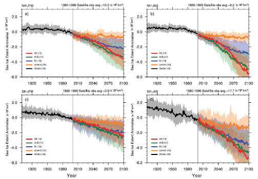
Figure 10.13. Multi-model simulated anomalies in sea ice extent for the 20th century (20c3m) and 21st century using the SRES A2, A1B and B1 as well as the commitment scenario for (a) Northern Hemisphere January to March (JFM), (b) Northern Hemisphere July to September (JAS). Panels (c) and (d) are as for (a) and (b) but for the Southern Hemisphere. The solid lines show the multi-model mean, shaded areas denote ±1 standard deviation. Sea ice extent is defined as the total area where sea ice concentration exceeds 15%. Anomalies are relative to the period 1980 to 2000 . The number of models is given in the legend and is different for each scenario.
An important characteristic of the projected change is for summer ice area to decline far more rapidly than winter ice area ( Gordon and O’Farrell, 1997 [JoC, MoS] ), and hence sea ice rapidly approaches a seasonal ice cover in both hemispheres (Figures 10.13 band 10.14). Seasonal ice cover is, however, rather robust and persists to some extent throughout the 21st century in most (if not all) models. Bitz and Roe 2004 [JoC, SRC] ) note that future projections show that arctic sea ice thins fastest where it is initially thickest, a characteristic that future climate projections share with sea ice thinning observed in the late 20th century ( Rothrock et al., 1999 [JoC, ARC] ). Consistent with these results, a projection by Gregory et al. 2002b [JoC, MoS, SRC] ) shows that arctic sea ice volume decreases more quickly than sea ice area (because trends in winter ice area are low) in the 21st century.
In 20th- and 21st-century simulations, antarctic sea ice cover is projected to decrease more slowly than in the Arctic (Figures 10.13 c,d and 10.14 ), particularly in the vicinity of the Ross Sea where most models predict a local minimum in surface warming. This is commensurate with the region with the greatest reduction in ocean heat loss, which results from reduced vertical mixing in the ocean ( Gregory, 2000 [JoC, SRC] ). The ocean stores much of its increased heat below 1 km depth in the Southern Ocean. In contrast, horizontal heat transport poleward of about 60°N increases in many models ( Holland and Bitz, 2003 [JoC, MoS, SRC] ), but much of this heat remains in the upper 1 km of the northern subpolar seas and Arctic Ocean ( Gregory, 2000 [JoC, SRC] ; Bitz et al., 2006 [JoC, SRC] Bitz et al. 2006 [JoC, SRC] ) argue that these differences in the depth where heat is accumulating in the high-latitude oceans have consequences for the relative rates of sea ice decay in the Arctic and Antarctic.
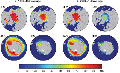
Figure 10.14. Multi-model mean sea ice concentration (%) for January to March (JFM) and June to September (JAS), in the Arctic (top) and Antarctic (bottom) for the periods (a) 1980 to 2000 and b) 2080 to 2100 for the SRES A1B scenario. The dashed white line indicates the present-day 15% average sea ice concentration limit. Modified from Flato et al. 2004 [JoC, MoS, ARC] ).
While most climate models share these common characteristics (peak surface warming in autumn and early winter, sea ice rapidly becomes seasonal, arctic ice decays faster than antarctic ice, and northward ocean heat transport increases into the northern high latitudes), models have poor agreement on the amount of thinning of sea ice (Flato and Participating CMIP Modeling Groups, 2004; Arzel et al., 2006 [JoC, MoS, ARC] ) and the overall climate change in the polar regions ( IPCC, 2001 [NPR] ; Holland and Bitz, 2003 [JoC, MoS, SRC] Flato 2004 [JoC, MoS, ARC] ) shows that the basic state of the sea ice and the reduction in thickness and/or extent have little to do with sea ice model physics among CMIP2 models. Holland and Bitz 2003 [JoC, MoS, SRC] and Arzel et al. 2006 [JoC, MoS, ARC] ) find serious biases in the basic state of simulated sea ice thickness and extent. Further, Rind et al. 1995 [JoC, MoS, ARC] Holland and Bitz 2003 [JoC, MoS, SRC] and Flato 2004 [JoC, MoS, ARC] ) show that the basic state of the sea ice thickness and extent have a significant influence on the projected change in sea ice thickness in the Arctic and extent in the Antarctic.
10.3.3.2 Changes in Snow Cover and Frozen Ground
Snow cover is an integrated response to both temperature and precipitation and exhibits strong negative correlation with air temperature in most areas with a seasonal snow cover (see Section 8.6.3.3 for an evaluation of model-simulated present-day snow cover). Because of this temperature association, the simulations project widespread reductions in snow cover over the 21st century (Supplementary Material, Figure S10.1). For the Arctic Climate Impact Assessment (ACIA) model mean, at the end of the 21st century the projected reduction in the annual mean NH snow cover is 13% under the B2 scenario ( ACIA, 2004 [NPR] ). The individual model projections range from reductions of 9 to 17%. The actual reductions are greatest in spring and late autumn/early winter, indicating a shortened snow cover season ( ACIA, 2004 [NPR] ). The beginning of the snow accumulation season (the end of the snowmelt season) is projected to be later (earlier), and the fractional snow coverage is projected to decrease during the snow season ( Hosaka et al., 2005 [MoS, SRC] ).
Warming at high northern latitudes in climate model simulations is also associated with large increases in simulated thaw depth over much of the permafrost regions ( Lawrence and Slater, 2005 [JoC, MoS, SRC] ; Yamaguchi et al., 2005 [MoS, SRC] ;( Kitabata et al., 2006 ) Yamaguchi et al. 2005 [MoS, SRC] ) show that initially soil moisture increases during the summer. In the late 21st century when the thaw depth has increased substantially, a reduction in summer soil moisture eventually occurs ( (Kitabata et al., 2006 ) Stendel and Christensen 2002 [JoC, ARC] ) show poleward movement of permafrost extent, and a 30 to 40% increase in active layer thickness for most of the permafrost area in the NH, with the largest relative increases concentrated in the northernmost locations.
Regionally, the changes are a response to both increased temperature and increased precipitation (changes in circulation patterns) and are complicated by the competing effects of warming and increased snowfall in those regions that remain below freezing (see Section 4.2 for a further discussion of processes that affect snow cover). In general, snow amount and snow coverage decreases in the NH (Supplementary Material, Figure S10.1). However, in a few regions (e.g., Siberia), snow amount is projected to increase. This is attributed to the increase in precipitation (snowfall) from autumn to winter ( (Meleshko et al., 2004; ) Hosaka et al., 2005 [MoS, SRC] ).
10.3.3.3 Changes in Greenland Ice Sheet Mass Balance
As noted in Section 10.6 ,modelling studies (e.g., Hanna et al., 2002 [MoS, SRC] ; Kiilsholm et al., 2003 [JoC, MoS, SRC] ; Wild et al., 2003 [JoC, SRC] ) as well as satellite observations, airborne altimeter surveys and other studies ( Abdalati et al., 2001 [JoC] ; Thomas et al., 2001 [JoC, ARC] ; Krabill et al., 2004 [JoC] ; Johannessen et al., 2005 [JoC] ;( Zwally et al., 2005; ) Rignot and Kanagaratnam, 2006 [JoC, ARC] ) suggest a slight inland thickening and strong marginal thinning resulting in an overall negative Greenland Ice Sheet mass balance which has accelerated recently (see Section 4.6.2.2 .). A consistent feature of all climate models is that projected 21st-century warming is amplified in northern latitudes. This suggests continued melting of the Greenland Ice Sheet, since increased summer melting dominates over increased winter precipitation in model projections of future climate. Ridley et al. 2005 [JoC, SRC] ) coupled UKMO-HadCM3 to an ice sheet model to explore the melting of the Greenland Ice Sheet under elevated (four times pre-industrial) levels of atmospheric CO2 (see Section 10.7.4.3 , Figure 10.38 ). While the entire Greenland Ice Sheet eventually completely ablated (after 3 kyr), the peak rate of melting was 0.06 Sv (1 Sv = 106 m3 s–1)corresponding to about 5.5 mm yr–1 global sea level rise (see Sections 10.3.4 and 10.6.6). Toniazzo et al. 2004 [JoC, SRC] ) further show that in UKMO-HadCM3, the complete melting of the Greenland Ice sheet is an irreversible process even if pre-industrial levels of atmospheric CO2 are re-established after it melts.
10.3.4 Changes in the Atlantic Meridional Overturning Circulation
Afeature common to all climate model projections is the increase in high-latitude temperature as well as an increase in high-latitude precipitation. This was reported in the TAR and is confirmed by the projections using the latest versions of comprehensive climate models (see Section 10.3.2 ). Both of these effects tend to make the high-latitude surface waters less dense and hence increase their stability, thereby inhibiting convective processes. As more coupled models have become available since the TAR, the evolution of the Atlantic Meridional Overturning Circulation (MOC) can be more thoroughly assessed. Figure 10.15 shows simulations from 19 coupled models integrated from 1850 to 2100 under SRES A1B atmospheric CO2 and aerosol scenarios up to year 2100, and constant concentrations thereafter (see Figure 10.5 ). All of the models, except CGCM3.1, INM-CM3.0 and MRI-CGCM2.3.2, were run without flux adjustments (see Table 8.1 ). The MOC is influenced by the density structure of the Atlantic Ocean, small-scale mixing and the surface momentum and buoyancy fluxes. Some models simulate a MOC strength that is inconsistent with the range of present-day estimates ( (Smethie and Fine, 2001; ) Ganachaud, 2003 [JoC, MoS] ;( Lumpkin and Speer, 2003; ) Talley, 2003 [ARC] ). The MOC for these models is shown for completeness but is not used in assessing potential future changes in the MOC in response to various emissions scenarios.
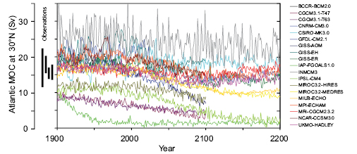
Figure 10.15. Evolution of the Atlantic meridional overturning circulation (MOC) at 30°N in simulations with the suite of comprehensive coupled climate models (see Table 8.1 for model details) from 1850 to 2100 using 20th Century Climate in Coupled Models (20C3M) simulations for 1850 to 1999 and the SRES A1B emissions scenario for 1999 to 2100 . Some of the models continue the integration to year 2200 with the forcing held constant at the values of year 2100 . Observationally based estimates of late-20th century MOC are shown as vertical bars on the left. Three simulations show a steady or rapid slow down of the MOC that is unrelated to the forcing; a few others have late-20th century simulated values that are inconsistent with observational estimates. Of the model simulations consistent with the late-20th century observational estimates, no simulation shows an increase in the MOC during the 21st century; reductions range from indistinguishable within the simulated natural variability to over 50% relative to the 1960 to 1990 mean; and none of the models projects an abrupt transition to an off state of the MOC. Adapted from Schmittner et al. 2005 [JoC, MoS, SRC] ) with additions.
Fewer studies have focused on projected changes in the Southern Ocean resulting from future climate warming. A common feature of coupled model simulations is the projected poleward shift and strengthening of the SH westerlies ( Yin, 2005 [JoC, MoS] ; Fyfe and Saenko, 2006 [JoC, MoS, ARC] ). This in turn leads to a strengthening, poleward shift and narrowing of the Antarctic Circumpolar Current. Fyfe and Saenko 2006 [JoC, MoS, ARC] ) further note that the enhanced equatorward surface Ekman transport, associated with the intensified westerlies, is balanced by an enhanced deep geostrophic poleward return flow below 2,000 m.
Generally, the simulated late-20th century Atlantic MOC shows a spread ranging from a weak MOC of about 12 Sv to over 20 Sv( Figure 10.15 ;Schmittner et al., 2005 [JoC, MoS, SRC] ). When forced with the SRES A1B scenario, the models show a reduction in the MOC of up to 50% or more, but in one model, the changes are not distinguishable from the simulated natural variability. The reduction in the MOC proceeds on the time scale of the simulated warming because it is a direct response to the increase in buoyancy at the ocean surface. A positive North Atlantic Oscillation (NAO) trend might delay this response by a few decades but not prevent it ( Delworth and Dixon, 2000 [JoC, SRC] ). Such a weakening of the MOC in future climate causes reduced sea surface temperature (SST) and salinity in the region of the Gulf Stream and North Atlantic Current ( Dai et al., 2005 [JoC, MoS, ARC] ). This can produce a decrease in northward heat transport south of 60°N, but increased northward heat transport north of 60°N (A. Hu et al., 2004 [Ambiguous] ). No model shows an increase in the MOC in response to the increase in greenhouse gases, and no model simulates an abrupt shut-down of the MOC within the 21st century. One study suggests that inherent low-frequency variability in the Atlantic region, the Atlantic Multidecadal Oscillation, may produce a natural weakening of the MOC over the next few decades that could further accentuate the decrease due to anthropogenic climate change ( Knight et al., 2005 [JoC] ; see Section 8.4.6 ).
In some of the older models (e.g., Dixon et al., 1999 [JoC, SRC] ), increased high-latitude precipitation dominates over increased high-latitude warming in causing the weakening, while in others (e.g., Mikolajewicz and Voss, 2000 [JoC] ), the opposite is found. In a recent model intercomparison, Gregory et al. 2005 [JoC, MoS, SRC] ) find that for all 11 models analysed, the MOC reduction is caused more by changes in surface heat flux than changes in surface freshwater flux. In addition, simulations using models of varying complexity ( Stocker et al., 1992b [JoC, MoS, SRC] ; Saenko et al., 2003 [JoC, SRC] ; Weaver et al., 2003 [JoC, SRC] ) show that freshening or warming in the Southern Ocean acts to increase or stabilise the Atlantic MOC. This is likely a consequence of the complex coupling of Southern Ocean processes with North Atlantic Deep Water production.
Afew simulations using coupled models are available that permit the assessment of the long-term stability of the MOC ( Stouffer and Manabe, 1999 [JoC, MoS, SRC] ; Voss and Mikolajewicz, 2001 [JoC, MoS] ; Stouffer and Manabe, 2003 [JoC, SRC] ; Wood et al., 2003 [JoC, ARC] ; Yoshida et al., 2005 [MoS] ; Bryan et al., 2006 [JoC] ). Most of these simulations assume an idealised increase in atmospheric CO2 by 1% yr–1 to various levels ranging from two to four times pre-industrial levels. One study also considers slower increases ( Stouffer and Manabe, 1999 [JoC, MoS, SRC] ), or a reduction in CO2 ( Stouffer and Manabe, 2003 [JoC, SRC] ). The more recent models are not flux adjusted and have higher resolution (about 1.0°) ( Yoshida et al., 2005 [MoS] ; Bryan et al., 2006 [JoC] ). A common feature of all simulations is a reduction in the MOC in response to the warming and a stabilisation or recovery of the MOC when the concentration is kept constant after achieving a level of two to four times the pre-industrial atmospheric CO2 concentration. None of these models shows a shutdown of the MOC that continues after the forcing is kept constant. But such a long-term shutdown cannot be excluded if the amount of warming and its rate exceed certain thresholds as shown using an EMIC ( Stocker and Schmittner, 1997 [JoC, SRC] ). Complete shut-downs, although not permanent, were also simulated by a flux-adjusted coupled model ( Manabe and Stouffer, 1994 [JoC, MoS, SRC] ; Stouffer and Manabe, 2003 [JoC, SRC] ; see also Chan and Motoi, 2005 [JoC] ). In none of these AOGCM simulations were the thresholds, as determined by the EMIC, passed ( Stocker and Schmittner, 1997 [JoC, SRC] ). As such, the long-term stability of the MOC found in the present AOGCM simulations is consistent with the results from the simpler models.
The reduction in MOC strength associated with increasing greenhouse gases represents a negative feedback for the warming in and around the North Atlantic. That is, through reducing the transport of heat from low to high latitudes, SSTs are cooler than they would otherwise be if the MOC was unchanged. As such, warming is reduced over and downstream of the North Atlantic. It is important to note that in models where the MOC weakens, warming still occurs downstream over Europe due to the overall dominant role of the radiative forcing associated with increasing greenhouse gases ( Gregory et al., 2005 [JoC, MoS, SRC] ). Many future projections show that once the radiative forcing is held fixed, re-establishment of the MOC occurs to a state similar to that of the present day. The partial or complete re-establishment of the MOC is slow and causes additional warming in and around the North Atlantic. While the oceanic meridional heat flux at low latitudes is reduced upon a slowdown of the MOC, many simulations show increasing meridional heat flux into the Arctic which contributes to accelerated warming and sea ice melting there. This is due to both the advection of warmer water and an intensification of the influx of North Atlantic water into the Arctic (A. Hu et al., 2004 [Ambiguous] ).
Climate models that simulated a complete shutdown of the MOC in response to sustained warming were flux-adjusted coupled GCMs or EMICs. A robust result from such simulations is that the shutdown of the MOC takes several centuries after the forcing is kept fixed (e.g., at 4 × atmospheric CO2 concentration). Besides the forcing amplitude and rate ( Stocker and Schmittner, 1997 [JoC, SRC] ), the amount of mixing in the ocean also appears to determine the stability of the MOC: increased vertical and horizontal mixing tends to stabilise the MOC and to eliminate the possibility of a second equilibrium state ( Manabe and Stouffer, 1999 [JoC, SRC] ; Knutti and Stocker, 2000 [JoC, SRC] ; Longworth et al., 2005 [JoC, SRC] ). Random internal variability or noise, often not present in simpler models, may also be important in determining the effective MOC stability ( Knutti and Stocker, 2002 [JoC, MoS, SRC] ; Monahan, 2002 [MoS, ARC] ).
The MOC is not necessarily a comprehensive indicator of ocean circulation changes in response to global warming. In a transient 2 × atmospheric CO2 experiment using a coupled AOGCM, the MOC changes were small, but convection in the Labrador Sea stopped due to warmer and hence less dense waters that inflow from the Greenland-Iceland-Norwegian Sea (GIN Sea) ( Wood et al., 1999 [JoC, MoS, SRC] ; Stouffer et al., 2006a [JoC, MoS, SRC] ). Similar results were found by A. Hu et al. 2004 [Ambiguous] ), who also report an increase in convection in the GIN Sea due to the influx of more saline waters from the North Atlantic. Various simulations using coupled models of different complexity find significant reductions in convection in the GIN Sea in response to warming ( Schaeffer et al., 2004 [JoC, MoS, ARC] ; Bryan et al., 2006 [JoC] ). Presumably, a delicate balance exists in the GIN Sea between the circum-arctic river runoff, sea ice production and advection of saline waters from the North Atlantic, and on a longer time scale, the inflow of freshwater through Bering Strait. The projected increases in circum-arctic river runoff ( Wu et al., 2005 [JoC, SRC] ) may enhance the tendency towards a reduction in GIN Sea convection ( Stocker and Raible, 2005 [JoC, SRC] ; Wu et al., 2005 [JoC, SRC] ). Cessation of convection in the Labrador Sea in the next few decades is also simulated in a high-resolution model of the Atlantic Ocean driven by surface fluxes from two AOGCMs ( Schweckendiek and Willebrand, 2005 [JoC, MoS, ARC] ). The large-scale responses of the high-resolution ocean model (e.g., MOC, Labrador Seas) agree with those from the AOGCMs. The grid resolution of the ocean components in the coupled AOGCMs has significantly increased since the TAR, and some consistent patterns of changes in convection and water mass properties in the Atlantic Ocean emerge in response to the warming, but models still show a variety of responses in the details.
The best estimate of sea level from 1993 to 2003 (see Section 5.5.5.2 )associated with the slight net negative mass balance from Greenland is 0.1 to 0.3 mm yr–1 over the total ocean surface. This converts to only about 0.002 to 0.003 Sv of freshwater forcing. Such an amount, even when added directly and exclusively to the North Atlantic, has been suggested to be too small to affect the North Atlantic MOC (see Weaver and Hillaire-Marcel, 2004a [SRC] ). While one model exhibits a MOC weakening in the later part of the 21st century due to Greenland Ice Sheet melting ( Fichefet et al., 2003 [JoC, ARC] ), this same model had a very large downward drift of its overturning in the control climate, making it difficult to actually attribute the model MOC changes to the ice sheet melting. As noted in Section 10.3.3.3 ,Ridley et al. 2005 [JoC, SRC] ) find the peak rate of Greenland Ice Sheet melting is about 0.1 Sv when they instantaneously elevate greenhouse gas levels in UKMO-HadCM3. They further note that this has little effect on the North Atlantic meridional overturning, although 0.1 Sv is sufficiently large to cause more dramatic transient changes in the strength of the MOC in other models ( Stouffer et al., 2006b [JoC, MoS, SRC] ).
Taken together, it is very likely that the MOC, based on currently available simulations, will decrease, perhaps associated with a significant reduction in Labrador Sea Water formation, but very unlikely that the MOC will undergo an abrupt transition during the course of the 21st century. At this stage, it is too early to assess the likelihood of an abrupt change of the MOC beyond the end of the 21st century, but the possibility cannot be excluded (see Box 10.1 ). The few available simulations with models of different complexity instead suggest a centennial slowdown. Recovery of the MOC is simulated in some models if the radiative forcing is stabilised but would take several centuries; in other models, the reduction persists.
Theory, models and palaeoclimatic reconstructions (see Chapter6 )have established the fact that changes in the climate system can be abrupt and widespread. A working definition of ‘abrupt climate change’ is given in Alley et al. (2002): ‘Technically, an abrupt climate change occurs when the climate system is forced to cross some threshold, triggering a transition to a new state at a rate determined by the climate system itself and faster than the cause’. More generally, a gradual change in some determining quantity of the climate system (e.g., radiation balance, land surface properties, sea ice, etc.) can cause a variety of structurally different responses( Box 10.1 ,Figure 1). The response of a purely linear system scales with the forcing, and at stabilisation of the forcing, a new equilibrium is achieved which is structurally similar, but not necessarily close to the original state. However, if the system contains more than one equilibrium state, transitions to structurally different states are possible. Upon the crossing of a tipping point (bifurcation point), the evolution of the system is no longer controlled by the time scale of the forcing, but rather determined by its internal dynamics, which can either be much faster than the forcing, or significantly slower. Only the former case would be termed ‘abrupt climate change’, but the latter case is of equal importance. For the long-term evolution of a climate variable one must distinguish between reversible and irreversible changes. The notion of ‘climate surprises’ usually refers to abrupt transitions and temporary or permanent transitions to a different state in parts of the climate system such as, for example, the 8.2 kyr event (see Section 6.5.2.1 ). The best-documented type of abrupt climate change in the palaeoclimatic archives is that associated with changes in the ocean circulation (Stocker, 2000). Since the TAR, many new results from climate models of different complexity have provided a more detailed view on the anticipated changes in the Atlantic MOC in response to global warming. Most models agree that the MOC weakens over the next 100 years and that this reduction ranges from indistinguishable from natural variability to over 50% by 2100( Figure 10.15 ). None of the AOGCM simulations shows an abrupt change when forced with the SRES emissions scenarios until 2100, but some long-term model simulations suggest that a complete cessation can result for large forcings (Stouffer and Manabe, 2003). Models of intermediate complexity indicate that thresholds in the MOC may be present but that they depend on the amount and rate of warming for a given model (Stocker and Schmittner, 1997). The few long-term simulations from AOGCMs indicate that even complete shutdowns of the MOC may be reversible (Stouffer and Manabe, 2003; Yoshida et al., 2005; Stouffer et al., 2006b). However, until millennial simulations with AOGCMs are available, the important question of potential irreversibility of an MOC shutdown remains unanswered. Both simplified models and AOGCMs agree, however, that a potentially complete shut-down of the MOC, induced by global warming, would take many decades to more than a century. There is no direct model evidence that the MOC could collapse within a few decades in response to global warming. However, a few studies do show the potential for rapid changes in the MOC (Manabe and Stouffer, 1999), and the processes concerned are poorly understood (see Section 8.7 ). This is not inconsistent with the palaeoclimate records. The cooling events during the last ice ages registered in the Greenland ice cores developed over a couple of centuries to millennia. In contrast, there were also a number of very rapid warmings, the so-called Dansgaard-Oeschger events (NorthGRIP Members, 2004), or rapid cooling (LeGrande et al., 2006), which evolved over decades or less, most probably associated with rapid latitudinal shifts in ocean convection sites and changes in strength of the MOC (see Section 6.3.2 ). Recent simulations with models with ocean components that resolve topography in sufficient detail obtain a consistent pattern of a strong to complete reduction of convection in the Labrador Sea (Wood et al., 1999; Schweckendiek and Willebrand, 2005). Such changes in the convection, with implications for the atmospheric circulation, can develop within a few years (Schaeffer et al., 2002). The long-term and regional-to-hemispheric scale effects of such changes in water mass properties have not yet been investigated. With a reduction in the MOC, the meridional heat flux also decreases in the subtropical and mid-latitudes with large-scale effects on the atmospheric circulation. In consequence, the warming of the North Atlantic surface proceeds more slowly. Even for strong reductions in MOC towards the end of the 21st century, no cooling is observed in the regions around the North Atlantic because it is overcompensated by the radiative forcing that caused the ocean response in the first place. At high latitudes, an increase in the oceanic meridional heat flux is simulated by these models. This increase is due to both an increase in the overturning circulation in the Arctic and the advection of warmer waters from lower latitudes and thus contributes significantly to continuing sea ice reduction in the Atlantic sector of the Arctic (A. Hu et al., 2004). Few simulations have also addressed the changes in overturning in the South Atlantic and Southern Ocean. In addition to water mass modifications, this also has an effect on the transport by the Antarctic Circumpolar Current, but results are not yet conclusive. Current understanding of the processes responsible for the initiation of an ice age indicate that a reduction or collapse of the MOC in response to global warming could not start an ice age (Berger and Loutre, 2002; Crucifix and Loutre, 2002; Yoshimori et al., 2002; Weaver and Hillaire-Marcel, 2004b).
Box 10.1, Figure 1. Schematic illustration of various responses of a climate variable to forcing. The forcing (top panels) reaches a new stable level (left part of figure), and later approaches the original level on very long time scales (right part of the figure). The response of the climate variable (bottom panels) can be smooth (solid line) or cross a tipping point inducing a transition to a structurally different state (dashed lines). That transition can be rapid (abrupt change, long-dashed), or gradual (short-dashed), but is usually dictated by the internal dynamics of the climate system rather than the forcing. The long-term behaviour (right part) also exhibits different possibilities. Changes can be irreversible (dash-dotted) with the system settling at a different stable state, or reversible (solid, dotted) when the forcing is set back to its original value. In the latter case, the transition again can be gradual or abrupt. An example for illustration, but not the only one, is the response of the Atlantic meridional overturning circulation to a gradual change in radiative forcing. Arctic sea ice is responding sensitively to global warming. While changes in winter sea ice cover are moderate, late summer sea ice is projected to disappear almost completely towards the end of the 21st century. A number of positive feedbacks in the climate system accelerate the melt back of sea ice. The ice-albedo feedback allows open water to receive more heat from the Sun during summer, and the increase in ocean heat transport to the Arctic through the advection of warmer waters and stronger circulation further reduces ice cover. Minimum arctic sea ice cover is observed in September. Model simulations indicate that the September sea ice cover decreases substantially in response to global warming, generally evolving on the time scale of the warming. With sustained warming, the late summer disappearance of a major fraction of arctic sea ice is permanent. Glaciers and ice caps are sensitive to changes in temperature and precipitation. Observations point to a reduction in volume over the last 20 years (see Section 4.5.2 ), with a rate during 1993 to 2003 corresponding to 0.77 ± 0.22 mm yr–1 sea level equivalent, with a larger mean central estimate than that for 1961 to 1998 (corresponding to 0.50 ± 0.18 mm yr–1 sea level equivalent). Rapid changes are therefore already underway and enhanced by positive feedbacks associated with the surface energy balance of shrinking glaciers and newly exposed land surface in periglacial areas. Acceleration of glacier loss over the next few decades is likely (see Section 10.6.3 ). Based on simulations of 11 glaciers in various regions, a volume loss of 60% of these glaciers is projected by the year 2050 (Schneeberger et al., 2003). Glaciated areas in the Americas are also affected. A comparative study including seven GCM simulations at 2 × atmospheric CO2 conditions inferred that many glaciers may disappear completely due to an increase in the equilibrium line altitude (Bradley et al., 2004). The disappearance of these ice bodies is much faster than a potential re-glaciation several centuries hence, and may in some areas be irreversible. Satellite and in situ measurement networks have demonstrated increasing melting and accelerated ice flow around the periphery of the Greenland Ice Sheet (GIS) over the past 25 years (see Section 4.6.2 ). The few simulations of long-term ice sheet simulations suggest that the GIS will significantly decrease in volume and area over the coming centuries if a warmer climate is maintained (Gregory et al., 2004a; Huybrechts et al., 2004; Ridley et al., 2005). A threshold of annual mean warming of 1.9°C to 4.6°C in Greenland has been estimated for elimination of the GIS (Gregory and Huybrechts, 2006; see section 10.7.3.3), a process which would take many centuries to complete. Even if temperatures were to decrease later, the reduction of the GIS to a much smaller extent might be irreversible, because the climate of an ice-free Greenland could be too warm for accumulation; however, this result is model dependent (see Section 10.7.3.3). The positive feedbacks involved here are that once the ice sheet gets thinner, temperatures in the accumulation region are higher, increasing the melting and causing more precipitation to fall as rain rather than snow; that the lower albedo of the exposed ice-free land causes a local climatic warming; and that surface melt water might accelerate ice flow (see Section 10.6.4.2 ). Acollapse of the West Antarctic Ice Sheet (WAIS) has been discussed as a potential response to global warming for many years (Bindschadler, 1998; Oppenheimer, 1998; Vaughan, 2007). A complete collapse would cause a global sea level rise of about 5 m. The observed acceleration of ice streams in the Amundsen Sea sector of the WAIS, the rapidity of propagation of this signal upstream and the acceleration of glaciers that fed the Larsen B Ice Shelf after its collapse have renewed these concerns (see Section 10.6.4.2 ). (continued) It is possible that the presence of ice shelves tends to stabilise the ice sheet, at least regionally. Therefore, a weakening or collapse of ice shelves, caused by melting on the surface or by melting at the bottom by a warmer ocean, might contribute to a potential destabilisation of the WAIS, which could proceed through the positive feedback of grounding-line retreat. Present understanding is insufficient for prediction of the possible speed or extent of such a collapse (see Box 4.1 and Section 10.7.3.4). Irreversible and relatively rapid changes in vegetation cover and composition have occurred frequently in the past. The most prominent example is the desertification of the Sahara region about 4 to 6 ka (Claussen et al., 1999). The reason for this behaviour is believed to lie in the limits of plant communities with respect to temperature and precipitation. Once critical levels are crossed, certain species can no longer compete within their ecosystem. Areas close to vegetation boundaries will experience particularly large and rapid changes due to the slow migration of these boundaries induced by global warming. A climate model simulation into the future shows that drying and warming in South America leads to a continuous reduction in the forest of Amazonia (Cox et al., 2000, 2004). While evolving continuously over the 21st century, such a change and ultimate disappearance could be irreversible, although this result could be model dependent since an analysis of 11 AOGCMs shows a wide range of future possible rainfall changes over the Amazon (Li et al., 2006). One of the possible ‘climate surprises’ concerns the role of the soil in the global carbon cycle. As the concentration of CO2 is increasing, the soil is acting, in the global mean, as a carbon sink by assimilating carbon due to accelerated growth of the terrestrial biosphere (see also Section 7.3.3.1.1 ). However, by about 2050, a model simulation suggests that the soil changes to a source of carbon by releasing previously accumulated carbon due to increased respiration (Cox et al., 2000) induced by increasing temperature and precipitation. This represents a positive feedback to the increase in atmospheric CO2.While different models agree regarding the sign of the feedback, large uncertainties exist regarding the strength (Cox et al., 2000; Dufresne et al., 2002; Friedlingstein et al., 2006). However, the respiration increase is caused by a warmer and wetter climate. The switch from moderate sink to strong source of atmospheric carbon is rather rapid and occurs within two decades (Cox et al., 2004), but the timing of the onset is uncertain (Huntingford et al., 2004). A model intercomparison reveals that once set in motion, the increase in respiration continues even after the CO2 levels are held constant (Cramer et al., 2001). Although considerable uncertainties still exist, it is clear that feedback mechanisms between the terrestrial biosphere and the physical climate system exist which can qualitatively and quantitatively alter the response to an increase in radiative forcing. Changes in weather patterns and regimes can be abrupt processes that might occur spontaneously due to dynamical interactions in the atmosphere-ice-ocean system, or manifest as the crossing of a threshold in the system due to slow external forcing. Such shifts have been reported in SST in the tropical Pacific, leading to a more positive ENSO phase (Trenberth, 1990), in the stratospheric polar vortex (Christiansen, 2003), in a shut-down of deep convection in the Greenland Sea (Bönisch et al., 1997; Ronski and Budeus, 2005) and in an abrupt freshening of the Labrador Sea (Dickson et al., 2002). In the latter, the freshening evolved throughout the entire depth but the shift in salinity was particularly rapid: the 34.87 psu isohaline plunged from seasonally surface to 1,600 metres within 2 years with no return since 1973. In a long, unforced model simulation, a period of a few decades with anomalously cold temperatures (up to 10 standard deviations below average) in the region south of Greenland was found (Hall and Stouffer, 2001). It was caused by persistent winds that changed the stratification of the ocean and inhibited convection, thereby reducing heat transfer from the ocean to the atmosphere. Similar results were found in a different model in which the major convection site in the North Atlantic spontaneously switched to a more southerly location for several decades to centuries (Goosse et al., 2002). Other simulations show that the slowly increasing radiative forcing is able to cause transitions in the convective activity in the Greenland-Iceland-Norwegian Sea that have an influence on the atmospheric circulation over Greenland and Western Europe (Schaeffer et al., 2002). The changes unfold within a few years and indicate that the system has crossed a threshold. Amulti-model analysis of regimes of polar variability (NAO, Arctic and Antarctic Oscillations) reveals that the simulated trends in the 21st century influence the Arctic and Antarctic Oscillations and point towards more zonal circulation (Rauthe et al., 2004). Temperature changes associated with changes in atmospheric circulation regimes such as the NAO can exceed in certain regions (e.g., Northern Europe) the long-term global warming that causes such inter-decadal regime shifts (Dorn et al., 2003). Box 10.1: Future Abrupt Climate Change, ‘Climate Surprises’, and Irreversible Changes
Atlantic Meridional Overturning Circulation and other ocean circulation changes:
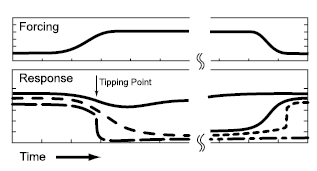
Arctic sea ice:
Glaciers and ice caps:
Greenland and West Antarctic Ice Sheets:
Vegetation cover:
Atmospheric and ocean-atmosphere regimes:
10.3.5 Changes in Properties of Modes of Variability
10.3.5.1 Interannual Variability in Surface Air Temperature and Precipitation
Future changes in anthropogenic forcing will result not only in changes in the mean climate state but also in the variability of climate. Addressing the interannual variability in monthly mean surface air temperature and precipitation of 19 AOGCMs in CMIP2, Räisänen 2002 [JoC, SRC] ) finds a decrease in temperature variability during the cold season in the extratropical NH and a slight increase in temperature variability in low latitudes and in warm season northern mid-latitudes. The former is likely due to the decrease of sea ice and snow with increasing temperature. The summer decrease in soil moisture over the mid-latitude land surfaces contributes to the latter. Räisänen 2002 [JoC, SRC] ) also finds an increase in monthly mean precipitation variability in most areas, both in absolute value (standard deviation) and in relative value (coefficient of variation). However, the significance level of these variability changes is markedly lower than that for time mean climate change. Similar results were obtained from 18 AOGCM simulations under the SRES A2 scenario ( Giorgi and Bi, 2005 [JoC, MoS, ARC] ).
10.3.5.2 Monsoons
In the tropics, an increase in precipitation is projected by the end of the 21st century in the Asian monsoon and the southern part of the West African monsoon with some decreases in the Sahel in northern summer ( Cook and Vizy, 2006 [JoC, MoS] ), as well as increases in the Australian monsoon in southern summer in a warmer climate( Figure 10.9 ). The monsoonal precipitation in Mexico and Central America is projected to decrease in association with increasing precipitation over the eastern equatorial Pacific that affects Walker Circulation and local Hadley Circulation changes( Figure 10.9 ). A more detailed assessment of regional monsoon changes is provided in Chapter 11 .
As a projected global warming will be more rapid over land than over the oceans, the continental-scale land-sea thermal contrast will become larger in summer and smaller in winter. Based on this, a simple idea is that the summer monsoon will be stronger and the winter monsoon will be weaker in the future than the present. However, model results are not as straightforward as this simple consideration. Tanaka et al. 2005 [MoS] ) define the intensities of Hadley, Walker and monsoon circulations using the velocity potential fields at 200 hPa. Using 15 AOGCMs, they show a weakening of these tropical circulations by 9%, 8% and 14%, respectively, by the late 21st century compared to the late 20th century. Using eight AOGCMs, Ueda et al. 2006 [JoC, MoS] ) demonstrate that pronounced warming over the tropics results in a weakening of the Asian summer monsoon circulations in relation to a reduction in the meridional thermal gradients between the Asian continent and adjacent oceans.
Despite weakening of the dynamical monsoon circulation, atmospheric moisture buildup due to increased greenhouse gases and consequent temperature increase results in a larger moisture flux and more precipitation for the Indian monsoon ( Douville et al., 2000 [MoS] ; IPCC, 2001 [NPR] ; Ashrit et al., 2003 [MoS] ; Meehl and Arblaster, 2003 [JoC, MoS, SRC] ; May, 2004; Ashrit et al., 2005 [MoS, SRC] ). For the South Asian summer monsoon, models suggest a northward shift of lower-tropospheric monsoon wind systems with a weakening of the westerly flow over the northern Indian Ocean ( Ashrit et al., 2003 [MoS] , 2005 ). Over Africa in northern summer, multi-model analysis projects an increase in rainfall in East and Central Africa, a decrease in the Sahel, and increases along the Gulf of Guinea coast( Figure 10.9 ). However, some individual models project an increase of rainfall in more extensive areas of West Africa related to a projected northward movement of the Sahara and the Sahel ( Liu et al., 2002 [JoC, MoS, SRC] ; Haarsma et al., 2005 [JoC] ). Whether the Sahel will be more or less wet in the future is thus uncertain, although a multi-model assessment of the West African monsoon indicates that the Sahel could become marginally more dry ( Cook and Vizy, 2006 [JoC, MoS] ). This inconsistency of the rainfall projections may be related to AOGCM biases, or an unclear relationship between Gulf of Guinea and Indian Ocean warming, land use change and the West African monsoon. Nonlinear feedbacks that may exist within the West African climate system should also be considered ( Jenkins et al., 2005 [JoC, MoS, SRC] ).
Most model results project increased interannual variability in season-averaged Asian monsoon precipitation associated with an increase in its long-term mean value (e.g., Hu et al., 2000b [JoC, MoS, SRC] ; Räisänen, 2002 [JoC, SRC] ; Meehl and Arblaster, 2003 [JoC, MoS, SRC] Hu et al. 2000a [JoC] ) relate this to increased variability in the tropical Pacific SST (El Niño variability) in their model. Meehl and Arblaster 2003 [JoC, MoS, SRC] ) relate the increased monsoon precipitation variability to increased variability in evaporation and precipitation in the Pacific due to increased SSTs. Thus, the South Asian monsoon variability is affected through the Walker Circulation such that the role of the Pacific Ocean dominates and that of the Indian Ocean is secondary.
Atmospheric aerosol loading affects regional climate and its future changes (see Chapter7 ). If the direct effect of the aerosol increase is considered, surface temperatures will not get as warm because the aerosols reflect solar radiation. For this reason, land-sea temperature contrast becomes smaller than in the case without the direct aerosol effect, and the summer monsoon becomes weaker. Model simulations of the Asian monsoon project that the sulphate aerosols’ direct effect reduces the magnitude of precipitation change compared with the case of only greenhouse gas increases ( Emori et al., 1999 [MoS, SRC] ; Roeckner et al., 1999 [JoC, MoS, SRC] ;( Lal and Singh, 2001 ) ). However, the relative cooling effect of sulphate aerosols is dominated by the effects of increasing greenhouse gases by the end of the 21st century in the SRES marker scenarios( Figure 10.26 ), leading to the increased monsoon precipitation at the end of the 21st century in these scenarios (see Section 10.3.2.3 ). Furthermore, it is suggested that aerosols with high absorptivity such as black carbon absorb solar radiation in the lower atmosphere, cool the surface, stabilise the atmosphere and reduce precipitation ( Ramanathan et al., 2001 [JoC, ARC] ). The solar radiation reaching the surface decreases as much as 50% locally, which could reduce the surface warming by greenhouse gases ( Ramanathan et al., 2005 [JoC, ARC] ). These atmospheric brown clouds could cause precipitation to increase over the Indian Ocean in winter and decrease in the surrounding Indonesia region and the western Pacific Ocean ( Chung et al., 2002 [Ambiguous] ), and could reduce the summer monsoon precipitation in South and East Asia ( Menon et al., 2002 [JoC, SRC] ; Ramanathan et al., 2005 [JoC, ARC] ). However, the total influence on monsoon precipitation of temporally varying direct and indirect effects of various aerosol species is still not resolved and the subject of active research.
10.3.5.3 Mean Tropical Pacific Climate Change
This subsection assesses changes in mean tropical Pacific climate. Enhanced greenhouse gas concentrations result in a general increase in SST, which will not be spatially uniform in association with a general reduction in tropical circulations in a warmer climate (see Section 10.3.5.2 ). Figures 10.8 and 10.9 indicate that SST increases more over the eastern tropical Pacific than over the western tropical Pacific, together with a decrease in the sea level pressure (SLP) gradient along the equator and an eastward shift of the tropical Pacific rainfall distribution. These background tropical Pacific changes can be called an El Niño-like mean state change (upon which individual El Niño-Southern Oscillation (ENSO) events occur). Although individual models show a large scatter of ‘ENSO-ness’ (Collins and The CMIP Modelling Groups, 2005; Yamaguchi and Noda, 2006 [SRC] ), an ENSO-like global warming pattern with positive polarity (i.e., El Niño-like mean state change) is simulated based on the spatial anomaly patterns of SST, SLP and precipitation( Figure 10.16 ;Yamaguchi and Noda, 2006 [SRC] ). The El Niño-like change may be attributable to the general reduction in tropical circulations resulting from the increased dry static stability in the tropics in a warmer climate ( Knutson and Manabe, 1995 [JoC, MoS, SRC] ; Sugi et al., 2002 [MoS, SRC] ; Figure 10.7 ). An eastward displacement of precipitation in the tropical Pacific accompanies an intensified and south-westward displaced subtropical anticyclone in the western Pacific, which can be effective in transporting moisture from the low latitudes to the Meiyu/Baiu region, thus generating more precipitation in the East Asian summer monsoon ( Kitoh and Uchiyama, 2006 [MoS, SRC] ).
In summary, the multi-model mean projects a weak shift towards conditions which may be described as ‘El Niño-like’, with SSTs in the central and eastern equatorial Pacific warming more than those in the west, and with an eastward shift in mean precipitation, associated with weaker tropical circulations.
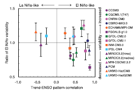
Figure 10.16. Base state change in average tropical Pacific SSTs and change in El Niño variability simulated by AOGCMs (see Table 8.1 for model details). The base state change (horizontal axis) is denoted by the spatial anomaly pattern correlation coefficient between the linear trend of SST in the 1% yr–1 CO2 increase climate change experiment and the first Empirical Orthogonal Function (EOF) of SST in the control experiment over the area 10°S to 10°N, 120°E to 80°W (reproduced from Yamaguchi and Noda, 2006 [SRC] ). Positive correlation values indicate that the mean climate change has an El Niño-like pattern, and negative values are la Niña-like. The change in El Niño variability (vertical axis) is denoted by the ratio of the standard deviation of the first EOF of sea level pressure (SLP) between the current climate and the last 50 years of the SRES A2 experiments ( 2051 – 2100 ), except for FGOALS-g1.0 and MIROC3.2(hires), for which the SRES A1B was used, and UKMO-HadGEM1 for which the 1% yr–1 CO2 increase climate change experiment was used, in the region 30°S to 30°N, 30°E to 60°W with a five-month running mean (reproduced from van Oldenborgh et al., 2005 [Ambiguous] ). Error bars indicate the 95% confidence interval. Note that tropical Pacific base state climate changes with either El Niño-like or La Niña-like patterns are not permanent El Niño or La Niña events, and all still have ENSO inter- annual variability superimposed on that new average climate state in a future warmer climate.
10.3.5.4 El Niño
This subsection addresses the projected change in the amplitude, frequency and spatial pattern of El Niño. Guilyardi 2006 [JoC, MoS] ) assessed mean state, coupling strength and modes (SST mode resulting from local SST-wind interaction or thermocline mode resulting from remote wind-thermocline feedbacks), using the pre-industrial control and stabilised 2 × and 4 × atmospheric CO2 simulations in a multi-model ensemble. The models that exhibit the largest El Niño amplitude change in scenario experiments are those that shift towards a thermocline mode. The observed 1976 climate shift in the tropical Pacific actually involved such a mode shift ( Fedorov and Philander, 2001 [JoC] ). The mean state change, through change in the sensitivity of SST variability to surface wind stress, plays a key role in determining the ENSO variance characteristics (Z. Hu et al., 2004 [Ambiguous] ; Zelle et al., 2005 [JoC, MoS] ). For example, a more stable ENSO system is less sensitive to changes in the background state than one that is closer to instability ( Zelle et al., 2005 [JoC, MoS] ). Thus, GCMs with an improper simulation of present-day climate mean state and air-sea coupling strength are not suitable for ENSO amplitude projections. van Oldenborgh et al. 2005 [Ambiguous] ) calculate the change in ENSO variability by the ratio of the standard deviation of the first Empirical Orthogonal Function (EOF) of SLP between the current climate and in the future( Figure 10.16 ), which shows that changes in ENSO interannual variability differ from model to model. They categorised 19 models based on their skill in the present-day ENSO simulations. Using the most realistic 6 out of 19 models, they find no statistically significant changes in the amplitude of ENSO variability in the future. Large uncertainty in the skewness of the variability limits the assessment of the future relative strength of El Niño and la Niña events. Merryfield 2006 [JoC, MoS] ) also analysed a multi-model ensemble and finds a wide range of behaviour for future El Niño amplitude, ranging from little change to larger El Niño events to smaller El Niño events, although several models that simulated some observed aspects of present-day El Niño events showed future increases in El Niño amplitude. However, significant multi-decadal fluctuations in El Niño amplitude in observations and in long coupled model control runs add another complicating factor to attempting to discern whether any future changes in El Niño amplitude are due to external forcing or are simply a manifestation of internal multi-decadal variability ( Meehl et al., 2006a [JoC, MoS, SRC] ). Even with the larger warming scenario under 4 × atmospheric CO2 climate, Yeh and Kirtman 2005 [JoC, ARC] ) find that despite the large changes in the tropical Pacific mean state, the changes in ENSO amplitude are highly model dependent. Therefore, there are no clear indications at this time regarding future changes in El Niño amplitude in a warmer climate. However, as first noted in the TAR, ENSO teleconnections over North America appear to weaken due at least in part to the mean change of base state mid-latitude atmospheric circulation ( Meehl et al., 2006a [JoC, MoS, SRC] ).
In summary, all models show continued ENSO interannual variability in the future no matter what the change in average background conditions, but changes in ENSO interannual variability differ from model to model. Based on various assessments of the current multi-model archive, in which present-day El Niño events are now much better simulated than in the TAR, there is no consistent indication at this time of discernible future changes in ENSO amplitude or frequency.
10.3.5.5 ENSO-Monsoon Relationship
The El Niño-Southern Oscillation affects interannual variability throughout the tropics through changes in the Walker Circulation. Analysis of observational data finds a significant correlation between ENSO and tropical circulation and precipitation such that there is a tendency for less Indian summer monsoon rainfall in El Niño years and above normal rainfall in La Niña years. Recent analyses have revealed that the correlation between ENSO and the Indian summer monsoon has decreased recently, and many hypotheses have been put forward (see Chapter3 ). With respect to global warming, one hypothesis is that the Walker Circulation (accompanying ENSO) shifted south-eastward, reducing downward motion in the Indian monsoon region, which originally suppressed precipitation in that region at the time of El Niño, but now produces normal precipitation as a result ( Krishna Kumar et al., 1999 [JoC] ). Another explanation is that as the ground temperature of the Eurasian continent has risen in the winter-spring season, the temperature difference between the continent and the ocean has increased, thereby causing more precipitation, and the Indian monsoon is normal in spite of the occurrence of El Niño ( Ashrit et al., 2001 [JoC] ).
An earlier version of an AOGCM developed at the Max Planck Institute (MPI) ( Ashrit et al., 2001 [JoC] ) and the Action de Recherche Petite Echelle Grande Echelle/Océan Parallélisé (ARPEGE/OPA) model ( Ashrit et al., 2003 [MoS] ) simulated no global-warming related change in the ENSO-monsoon relationship, although a decadal-scale fluctuation is seen, suggesting that a weakening of the relationship might be part of the natural variability. However, Ashrit et al. 2001 [JoC] ) show that while the impact of La Niña does not change, the influence of El Niño on the monsoon becomes small, suggesting the possibility of asymmetric behaviour of the changes in the ENSO-monsoon relationship. On the other hand, the MRI-CGCM2 (see Table 8.1 for model details) indicates a weakening of the correlation into the 21st century, particularly after 2050 ( Ashrit et al., 2005 [MoS, SRC] ). The MRI-CGCM2 model results support the above hypothesis that the Walker Circulation shifts eastward and no longer influences India at the time of El Niño in a warmer climate. Camberlin et al. 2004 [JoC, MoS] and van Oldenborgh and Burgers 2005 [JoC] ) find decadal fluctuations in the effect of ENSO on regional precipitation. In most cases, these fluctuations may reflect natural variability in the ENSO teleconnection, and long-term correlation trends may be comparatively weaker.
The Tropospheric Biennial Oscillation (TBO) has been suggested as a fundamental set of coupled interactions in the Indo-Pacific region that encompasses ENSO and the Asian-Australian monsoon, and the TBO has been shown to be simulated by current AOGCMs (see Chapter8 Nanjundiah et al. 2005 [MoS, ARC] ) analyse a multi-model data set to show that, for models that successfully simulate the TBO for present-day climate, the TBO becomes more prominent in a future warmer climate due to changes in the base state climate, although, as with ENSO, there is considerable inherent decadal variability in the relative dominance of TBO and ENSO.
In summary, the ENSO-monsoon relationship can vary due to natural variability. Model projections suggest that a future weakening of the ENSO-monsoon relationship could occur in a future warmer climate.
10.3.5.6 Annular Modes and Mid-Latitude Circulation Changes
Many simulations project some decrease in the arctic surface pressure in the 21st century, as seen in the multi-model average (see Figure 10.9 ). This contributes to an increase in indices of the Northern Annular Mode (NAM) or the Arctic Oscillation (AO), as well as the NAO, which is closely related to the NAM in the Atlantic sector (see Chapter8 ). In the recent multi-model analyses, more than half of the models exhibit a positive trend in the NAM ( Rauthe et al., 2004 [JoC, MoS] ; Miller et al., 2006 [PoC, JoC, MoS, SRC] ) and/or NAO ( Osborn, 2004 [PoC, JoC, MoS, ARC] ; Kuzmina et al., 2005 [JoC, MoS] ). Although the magnitude of the trends shows a large variation among different models, Miller et al. 2006 [PoC, JoC, MoS, SRC] ) find that none of the 14 models exhibits a trend towards a lower NAM index and higher arctic SLP. In another multi-model analysis, Stephenson et al. 2006 [JoC, MoS] ) show that of the 15 models able to simulate the NAO pressure dipole, 13 predict a positive increase in the NAO index with increasing CO2 concentrations, although the magnitude of the response is generally small and model dependent. However, the multi-model average from the larger number (21) of models shown in Figure 10.9 indicates that it is likely that the NAM index would not notably decrease in a future warmer climate. The average of IPCC-AR4 simulations from 13 models suggests the increase of the NAM index becomes statistically significant early in the 21st century( Figure 10.17 a, Miller et al., 2006 [PoC, JoC, MoS, SRC] ).
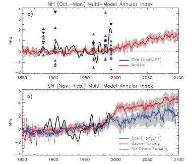
Figure 10.17. (a) Multi-model mean of the regression of the leading EOF of ensemble mean Northern Hemisphere sea level pressure (NH SLP, thin red line). The time series of regression coefficients has zero mean between year 1900 and 1970 . The thick red line is a 10-year low-pass filtered version of the mean. The grey shading represents the inter-model spread at the 95% confidence level and is filtered. A filtered version of the observed SLP from the Hadley Centre (HadSLP1) is shown in black. The regression coefficient for the winter following a major tropical eruption is marked by red, blue and black triangles for the multi-model mean, the individual model mean and observations, respectively. (b) As in (a) for Southern Hemisphere SLP for models with (red) and without (blue) ozone forcing. Adapted from Miller et al. 2006 [PoC, JoC, MoS, SRC] ).
The spatial patterns of the simulated SLP trends vary among different models, in spite of close correlations of the models’ leading patterns of interannual (or internal) variability with the observations ( Osborn, 2004 [PoC, JoC, MoS, ARC] ; Miller et al., 2006 [PoC, JoC, MoS, SRC] ). However, at the hemispheric scale of SLP change, the reduction in the Arctic is seen in the multi-model mean( Figure 10.9 ), although the change is smaller than the inter-model standard deviation. Besides the decrease in the arctic region, increases over the North Pacific and the Mediterranean Sea exceed the inter-model standard deviation; the latter suggests an association with a north-eastward shift of the NAO’s centre of action ( Hu and Wu, 2004 [JoC, MoS] ). The diversity of the patterns seems to reflect different responses in the Aleutian Low ( Rauthe et al., 2004 [JoC, MoS] ) in the North Pacific. Yamaguchi and Noda 2006 [SRC] ) discuss the modelled response of ENSO versus AO, and find that many models project a positive AO-like change. In the North Pacific at high latitudes, however, the SLP anomalies are incompatible between the El Niño-like change and the positive AO-like change, because models that project an El Niño-like change over the Pacific simulate a non-AO-like pattern in the polar region. As a result, the present models cannot fully determine the relative importance of the mechanisms inducing the positive AO-like change and those inducing the ENSO-like change, leading to scatter in global warming patterns at regional scales over the North Pacific. Rauthe et al. 2004 [JoC, MoS] ) suggest that the effects of sulphate aerosols contribute to a deepening of the Aleutian Low resulting in a slower or smaller increase in the AO index.
Analyses of results from various models indicate that the NAM can respond to increasing greenhouse gas concentrations through tropospheric processes ( Fyfe et al., 1999 [JoC, ARC] ; Gillett et al., 2003 [Ambiguous] ; Miller et al., 2006 [PoC, JoC, MoS, SRC] ). Greenhouse gases can also drive a positive NAM trend through changes in the stratospheric circulation, similar to the mechanism by which volcanic aerosols in the stratosphere force positive annular changes ( Shindell et al., 2001 [PoC, JoC, MoS, SRC] ). Models with their upper boundaries extending farther into the stratosphere exhibit, on average, a relatively larger increase in the NAM index and respond consistently to the observed volcanic forcing( Figure 10.17 a, Miller et al., 2006 [PoC, JoC, MoS, SRC] ), implying the importance of the connection between the troposphere and the stratosphere.
Aplausible explanation for the cause of the upward NAM trend simulated by the models is an intensification of the polar vortex resulting from both tropospheric warming and stratospheric cooling mainly due to the increase in greenhouse gases ( Shindell et al., 2001 [PoC, JoC, MoS, SRC] ; Sigmond et al., 2004 [JoC, MoS, ARC] ; Rind et al., 2005a [JoC, ARC] ). The response may not be linear with the magnitude of radiative forcing ( Gillett et al., 2002 [JoC, ARC] ) since the polar vortex response is attributable to an equatorward refraction of planetary waves ( Eichelberger and Holton, 2002 [JoC, MoS] ) rather than radiative forcing itself. Since the long-term variation in the NAO is closely related to SST variations ( Rodwell et al., 1999 [PoC, JoC, MoS, ARC] ), it is considered essential that the projection of the changes in the tropical SST ( Hoerling et al., 2004 [JoC] ; Hurrell et al., 2004 [JoC, ARC] ) and/or meridional gradient of the SST change ( Rind et al., 2005b [JoC, ARC] ) is reliable.
The future trend in the Southern Annular Mode (SAM) or the Antarctic Oscillation (AAO) has been projected in a number of model simulations ( Gillett and Thompson, 2003 [JoC, MoS, ARC] ; Shindell and Schmidt, 2004 [PoC, JoC, SRC] ; Arblaster and Meehl, 2006 [JoC, MoS, SRC] ; Miller et al., 2006 [PoC, JoC, MoS, SRC] ). According to the latest multi-model analysis ( Miller et al., 2006 [PoC, JoC, MoS, SRC] ), most models indicate a positive trend in the SAM index, and a declining trend in the antarctic SLP (as seen in Figure 10.9 ), with a higher likelihood than for the future NAM trend. On average, a larger positive trend is projected during the late 20th century by models that include stratospheric ozone changes than those that do not( Figure 10.17 b), although during the 21st century, when ozone changes are smaller, the SAM trends of models with and without ozone are similar. The cause of the positive SAM trend in the second half of the 20th century is mainly attributed to stratospheric ozone depletion, evidenced by the fact that the signal is largest in the lower stratosphere in austral spring through summer ( Thompson and Solomon, 2002 [PoC, JoC, ARC] ; Arblaster and Meehl, 2006 [JoC, MoS, SRC] ). However, increases in greenhouse gases are also important factors ( Shindell and Schmidt, 2004 [PoC, JoC, SRC] ; Arblaster and Meehl, 2006 [JoC, MoS, SRC] ) for the year-round positive SAM trend induced by meridional temperature gradient changes ( Brandefelt and Källén, 2004 [JoC, MoS] ). During the 21st century, although the ozone amount is expected to stabilise or recover, the polar vortex intensification is likely to continue due to the increases in greenhouse gases ( Arblaster and Meehl, 2006 [JoC, MoS, SRC] ).
It is implied that the future change in the annular modes leads to modifications of the future change in various fields such as surface temperatures, precipitation and sea ice with regional features similar to those for the modes of natural variability (e.g., Hurrell et al., 2003 [NPR, ARC] ). For instance, the surface warming in winter would be intensified in northern Eurasia and most of North America while weakened in the western North Atlantic, and winter precipitation would increase in northern Europe while decreasing in southern Europe. The atmospheric circulation change would also affect the ocean circulations. Sakamoto et al. 2005 [JoC, MoS] ) simulate an intensification of the Kuroshio Current but no shift in the Kuroshio Extension in response to an AO-like circulation change for the 21st century. However, Sato et al. 2006 [MoS] ) simulate a northward shift of the Kuroshio Extension, which leads to a strong warming off the eastern coast of Japan.
In summary, the future changes in the extratropical circulation variability are likely to be characterised by increases in positive phases of both the NAM and the SAM. The response in the NAM to anthropogenic forcing might not be distinct from the larger multi-decadal internal variability in the first half of the 21st century. The change in the SAM would appear earlier than in the NAM since stratospheric ozone depletion acts as an additional forcing. The positive trends in annular modes would influence the regional changes in temperature, precipitation and other fields, similar to those that accompany the NAM and the SAM in the present climate, but would be superimposed on the global-scale changes in a future warmer climate.
10.3.6 Future Changes in Weather and Climate Extremes
Projections of future changes in extremes rely on an increasingly sophisticated set of models and statistical techniques. Studies assessed in this section rely on multi-member ensembles (three to five members) from single models, analyses of multi-model ensembles ranging from 8 to 15 or more AOGCMs, and a perturbed physics ensemble with a single mixed-layer model with over 50 members. The discussion here is intended to identify general characteristics of changes in extremes in a global context. Chapter3 provides a definition of weather and climate extremes, and Chapter 11 addresses changes in extremes for specific regions.
10.3.6.1 Precipitation Extremes
Along-standing result from global coupled models noted in the TAR is a projected increase in the chance of summer drying in the mid-latitudes in a future warmer climate with associated increased risk of drought. This is shown in Figure 10.12 ,and has been documented in the more recent generation of models ( Burke et al., 2006 [JoC, MoS] ; Meehl et al., 2006b [JoC, MoS, SRC] ; Rowell and Jones, 2006 [JoC, MoS, ARC] ). For example, Wang 2005 [JoC, MoS] ) analyse 15 recent AOGCMs and show that in a future warmer climate, the models simulate summer dryness in most parts of the northern subtropics and mid-latitudes, but with a large range in the amplitude of summer dryness across models. Droughts associated with this summer drying could result in regional vegetation die-offs ( Breshears et al., 2005 [JoC] ) and contribute to an increase in the percentage of land area experiencing drought at any one time, for example, extreme drought increasing from 1% of present-day land area to 30% by the end of the century in the A2 scenario ( Burke et al., 2006 [JoC, MoS] ). Drier soil conditions can also contribute to more severe heat waves as discussed in Section 10.3.6.2 ( Brabson et al., 2005 [JoC, MoS, ARC] ).
Associated with the risk of drying is a projected increase in the chance of intense precipitation and flooding. Although somewhat counter-intuitive, this is because precipitation is projected to be concentrated into more intense events, with longer periods of little precipitation in between. Therefore, intense and heavy episodic rainfall events with high runoff amounts are interspersed with longer relatively dry periods with increased evapotranspiration, particularly in the subtropics as discussed in Section 10.3.6.2 in relation to Figure 10.19 ( Frei et al., 1998 [JoC, ARC] ; Allen and Ingram, 2002 [JoC, MoS, SRC] ; Palmer and Räisänen, 2002 [JoC, SRC] ; Christensen and Christensen, 2003 [JoC, ARC] ; Beniston, 2004 [JoC, MoS, ARC] ; Christensen and Christensen, 2004 [JoC, ARC] ; Pal et al., 2004 [JoC, MoS, ARC] ; Meehl et al., 2005a [JoC, MoS, SRC] ). However, increases in the frequency of dry days do not necessarily mean a decrease in the frequency of extreme high rainfall events depending on the threshold used to define such events ( Barnett et al., 2006 [JoC, MoS] ). Another aspect of these changes has been related to the mean changes in precipitation, with wet extremes becoming more severe in many areas where mean precipitation increases, and dry extremes where the mean precipitation decreases ( Kharin and Zwiers, 2005 [JoC, MoS, ARC] ; Meehl et al., 2005a [JoC, MoS, SRC] ; Räisänen, 2005a [JoC, SRC] ; Barnett et al., 2006 [JoC, MoS] ). However, analysis of the 53-member perturbed physics ensemble indicates that the change in the frequency of extreme precipitation at an individual location can be difficult to estimate definitively due to model parametrization uncertainty ( Barnett et al., 2006 [JoC, MoS] ). Some specific regional aspects of these changes in precipitation extremes are discussed further in Chapter 11 .
Climate models continue to confirm the earlier results that in a future climate warmed by increasing greenhouse gases, precipitation intensity (e.g., proportionately more precipitation per precipitation event) is projected to increase over most regions ( Wilby and Wigley, 2002 [PoC, JoC, MoS, SRC] ; Kharin and Zwiers, 2005 [JoC, MoS, ARC] ; Meehl et al., 2005a [JoC, MoS, SRC] ; Barnett et al., 2006 [JoC, MoS] ), and the increase in precipitation extremes is greater than changes in mean precipitation ( Kharin and Zwiers, 2005 [JoC, MoS, ARC] ). As discussed in Chapter9 ,this is related to the fact that the energy budget of the atmosphere constrains increases in large-scale mean precipitation, but extreme precipitation relates to increases in moisture content and thus the nonlinearities involved with the Clausius-Clapeyron relationship such that, for a given increase in temperature, increases in extreme precipitation can be more than the mean precipitation increase (e.g., Allen and Ingram, 2002 [JoC, MoS, SRC] ). Additionally, time scale can play a role whereby increases in the frequency of seasonal mean rainfall extremes can be greater than the increases in the frequency of daily extremes ( Barnett et al., 2006 [JoC, MoS] ). The increase in mean and extreme precipitation in various regions has been attributed to contributions from both dynamic and thermodynamic processes associated with global warming ( Emori and Brown, 2005 [JoC, SRC] ). The greater increase in extreme precipitation compared to the mean is attributed to the greater thermodynamic effect on the extremes due to increases in water vapour, mainly over subtropical areas. The thermodynamic effect is important nearly everywhere, but changes in circulation also contribute to the pattern of precipitation intensity changes at middle and high latitudes ( Meehl et al., 2005a [JoC, MoS, SRC] Kharin and Zwiers 2005 [JoC, MoS, ARC] ) show that changes in both the location and scale of the extreme value distribution produce increases in precipitation extremes substantially greater than increases in annual mean precipitation. An increase in the scale parameter from the gamma distribution represents an increase in precipitation intensity, and various regions such as the NH land areas in winter showed particularly high values of increased scale parameter ( Semenov and Bengtsson, 2002 [JoC, MoS] ; Watterson and Dix, 2003 [JoC, MoS, SRC] ). Time-slice simulations with a higher-resolution model (~1°) show similar results using changes in the gamma distribution, namely increased extremes in the hydrological cycle ( Voss et al., 2002 [JoC, MoS, SRC] ). However, some regional decreases are also projected such as over the subtropical oceans ( Semenov and Bengtsson, 2002 [JoC, MoS] ).
Anumber of studies have noted the connection between increased rainfall intensity and an implied increase in flooding. McCabe et al. 2001 [JoC] and Watterson 2005 [MoS, SRC] ) show a projected increase in extreme rainfall intensity with the extra-tropical surface lows, particularly over NH land, with an implied increase in flooding. In a multi-model analysis of the CMIP models, Palmer and Räisänen 2002 [JoC, SRC] ) show an increased likelihood of very wet winters over much of central and northern Europe due to an increase in intense precipitation associated with mid-latitude storms, suggesting more floods across Europe (see also Chapter 11 ). They found similar results for summer precipitation with implications for greater flooding in the Asian monsoon region in a future warmer climate. Similarly, Milly et al. 2002 [JoC, ARC] Arora and Boer 2001 [JoC, MoS, ARC] and Voss et al. 2002 [JoC, MoS, SRC] ) relate the increased risk of floods in a number of major river basins in a future warmer climate to an increase in spring river discharge related to increased winter snow depth in some regions. Christensen and Christensen 2003 [JoC, ARC] ) conclude that there could be an increased risk of summer flooding in Europe.
Globally averaged time series of the ( Frich et al. 2002 ) ) indices in the multi-model analysis of Tebaldi et al. 2006 [JoC, MoS, SRC] ) show simulated increases in precipitation intensity during the 20th century continuing through the 21st century( Figure 10.18 a,b), along with a somewhat weaker and less consistent trend of increasing dry periods between rainfall events for all scenarios( Figure 10.18 c,d). Part of the reason for these results is shown in the geographic maps for these quantities, where precipitation intensity increases almost everywhere, but particularly at middle and high latitudes where mean precipitation also increases ( Meehl et al., 2005a [JoC, MoS, SRC] ; compare Figure 10.18 bto Figure 10.9 ). However, in Figure 10.18 d, there are regions of increased runs of dry days between precipitation events in the subtropics and lower mid-latitudes, but decreased runs of dry days at higher mid-latitudes and high latitudes where mean precipitation increases (compare Figure 10.9 with Figure 10.18 d). Since there are areas of both increases and decreases in consecutive dry days between precipitation events in the multi-model average( Figure 10.9 ), the global mean trends are smaller and less consistent across models as shown in Figure 10.18 .Consistency of response in a perturbed physics ensemble with one model shows only limited areas of increased frequency of wet days in July, and a larger range of changes in precipitation extremes relative to the control ensemble mean in contrast to the more consistent response of temperature extremes( Section 10.6.3.2 ), indicating a less consistent response for precipitation extremes in general compared to temperature extremes ( Barnett et al., 2006 [JoC, MoS] ). Analysis of the ( Frich et al. 2002 ) ) precipitation indices in a 20-km resolution global model shows similar results to those in Figure 10.18 ,with particularly large increases in precipitation intensity in South Asia and West Africa ( Kamiguchi et al., 2005 [MoS] ).
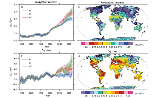
Figure 10.18. Changes in extremes based on multi-model simulations from nine global coupled climate models, adapted from Tebaldi et al. 2006 [JoC, MoS, SRC] ). (a) Globally averaged changes in precipitation intensity (defined as the annual total precipitation divided by the number of wet days) for a low (SRES B1), middle (SRES A1B) and high (SRES A2) scenario. (b) Changes in spatial patterns of simulated precipitation intensity between two 20-year means ( 2080 – 2099 minus 1980 – 1999 ) for the A1B scenario. (c) Globally averaged changes in dry days (defined as the annual maximum number of consecutive dry days). (d) Changes in spatial patterns of simulated dry days between two 20-year means ( 2080 – 2099 minus 1980 – 1999 ) for the A1B scenario. Solid lines in (a) and (c) are the 10-year smoothed multi-model ensemble means; the envelope indicates the ensemble mean standard deviation. Stippling in (b) and (d) denotes areas where at least five of the nine models concur in determining that the change is statistically significant. Extreme indices are calculated only over land following ( Frich et al. 2002 ) ). Each model’s time series was centred on its 1980 to 1999 average and normalised (rescaled) by its standard deviation computed (after de-trending) over the period 1960 to 2099 . The models were then aggregated into an ensemble average, both at the global and at the grid-box level. Thus, changes are given in units of standard deviations.
10.3.6.2 Temperature Extremes
The TAR concluded that there was a very likely risk of increased high temperature extremes (and reduced risk of low temperature extremes) with more extreme heat episodes in a future climate. The latter result has been confirmed in subsequent studies ( Yonetani and Gordon, 2001 [JoC, MoS] Kharin and Zwiers 2005 [JoC, MoS, ARC] ) show in a single model that future increases in temperature extremes follow increases in mean temperature over most of the world except where surface properties change (melting snow, drying soil). Furthermore, they show that in most instances warm extremes correspond to increases in daily maximum temperature, but cold extremes warm up faster than daily minimum temperatures, although this result is less consistent when model parameters are varied in a perturbed physics ensemble where there are increased daily temperature maxima for nearly the entire land surface. However, the range in magnitude of increases was substantial indicating a sensitivity to model formulations ( Clark et al., 2006 [JoC, MoS, SRC] ).
Weisheimer and Palmer 2005 [JoC, SRC] ) examine changes in extreme seasonal (DJF and JJA) temperatures in 14 models for three scenarios. They show that by the end of 21st century, the probability of such extreme warm seasons is projected to rise in many areas. This result is consistent with the perturbed physics ensemble where, for nearly all land areas, extreme JJA temperatures were at least 20 times and in some areas 100 times more frequent compared to the control ensemble mean, making these changes greater than the ensemble spread.
Since the TAR, possible future cold air outbreaks have been studied. Vavrus et al. 2006 [JoC, ARC] ) analyse seven AOGCMs run with the A1B scenario, and define a cold air outbreak as two or more consecutive days when the daily temperatures are at least two standard deviations below the present-day winter mean. For a future warmer climate, they document a 50 to 100% decline in the frequency of cold air outbreaks in NH winter in most areas compared to the present, with the smallest reductions occurring in western North America, the North Atlantic and southern Europe and Asia due to atmospheric circulation changes associated with the increase in greenhouse gases.
No studies at the time of the TAR specifically documented changes in heat waves (very high temperatures over a sustained period of days, see Chapter3 ). Several recent studies address possible future changes in heat waves explicitly, and find an increased risk of more intense, longer-lasting and more frequent heat waves in a future climate ( Meehl and Tebaldi, 2004 [JoC, SRC] ; Schär et al., 2004 [JoC, ARC] ; Clark et al., 2006 [JoC, MoS, SRC] Meehl and Tebaldi 2004 [JoC, SRC] ) show that the pattern of future changes in heat waves, with greatest intensity increases over western Europe, the Mediterranean and the southeast and western USA, is related in part to base state circulation changes due to the increase in greenhouse gases. An additional factor leading to extreme heat is drier soils in a future warmer climate ( Brabson et al., 2005 [JoC, MoS, ARC] ; Clark et al., 2006 [JoC, MoS, SRC] Schär et al. 2004 [JoC, ARC] Stott et al. 2004 [JoC, SRC] and Beniston 2004 [JoC, MoS, ARC] ) use the European 2003 heat wave as an example of the types of heat waves that are likely to become more common in a future warmer climate. Schär et al. 2004 [JoC, ARC] ) note that the increase in the frequency of extreme warm conditions is also associated with a change in interannual variability, such that the statistical distribution of mean summer temperatures is not merely shifted towards warmer conditions but also becomes wider. A multi-model ensemble shows that heat waves are simulated to have been increasing over the latter part of the 20th century, and are projected to increase globally and over most regions( Figure 10.19 ;Tebaldi et al., 2006 [JoC, MoS, SRC] ), although different model parameters can contribute to the range in the magnitude of this response ( Clark et al., 2006 [JoC, MoS, SRC] ).
Adecrease in DTR in most regions in a future warmer climate was reported in the TAR, and is substantiated by more recent studies (e.g., Stone and Weaver, 2002 [JoC, MoS, SRC] ; also discussed in relation to Figure 10.11 band in Chapter 11 ). For a quantity related to the DTR, the TAR concluded that it would be likely that a future warmer climate would also be characterised by a decrease in the number of frost days, although there were no studies at that time from global coupled climate models that addressed this issue explicitly. It has since been shown that there would indeed be decreases in frost days in a future warmer climate in the extratropics ( Meehl et al., 2004a [JoC, MoS, SRC] ), with the pattern of the decreases dictated by the changes in atmospheric circulation due to the increase in greenhouse gases ( Meehl et al., 2004a [JoC, MoS, SRC] ). Results from a nine-member multi-model ensemble show simulated decreases in frost days for the 20th century continuing into the 21st century globally and in most regions( Figure 10.19 ). A quantity related to frost days in many mid- and high-latitude areas, particularly in the NH, is growing season length as defined by ( Frich et al. 2002 ) ), and this has been projected to increase in future climate ( Tebaldi et al., 2006 [JoC, MoS, SRC] ). This result is also shown in a nine-member multi-model ensemble where the simulated increase in growing season length in the 20th century continues into the 21st century globally and in most regions( Figure 10.19 ). The globally averaged extremes indices in Figures 10.18 and 10.19 have non-uniform changes across the scenarios compared to the more consistent relative increases in Figure 10.5 for globally averaged temperature. This indicates that patterns that scale well by radiative forcing for temperature (e.g., Figure 10.8 )would not scale for extremes.
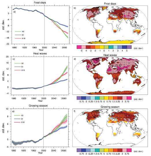
Figure 10.19. Changes in extremes based on multi-model simulations from nine global coupled climate models, adapted from Tebaldi et al. 2006 [JoC, MoS, SRC] ). (a) Globally averaged changes in the frost day index (defined as the total number of days in a year with absolute minimum temperature below 0°C) for a low (SRES B1), middle (SRES A1B) and high (SRES A2) scenario. (b) Changes in spatial patterns of simulated frost days between two 20-year means ( 2080 – 2099 minus 1980 – 1999 ) for the A1B scenario. (c) Globally averaged changes in heat waves (defined as the longest period in the year of at least five consecutive days with maximum temperature at least 5°C higher than the climatology of the same calendar day). (d) Changes in spatial patterns of simulated heat waves between two 20-year means ( 2080 – 2099 minus 1980 – 1999 ) for the A1B scenario. (e) Globally averaged changes in growing season length (defined as the length of the period between the first spell of five consecutive days with mean temperature above 5°C and the last such spell of the year). (f) Changes in spatial patterns of simulated growing season length between two 20-year means ( 2080 – 2099 minus 1980 – 1999 ) for the A1B scenario. Solid lines in (a), (c) and (e) show the 10-year smoothed multi-model ensemble means; the envelope indicates the ensemble mean standard deviation. Stippling in (b), (d) and (f) denotes areas where at least five of the nine models concur in determining that the change is statistically significant. Extreme indices are calculated only over land. Frost days and growing season are only calculated in the extratropics. Extremes indices are calculated following ( Frich et al. 2002 ) ). Each model’s time series was centred around its 1980 to 1999 average and normalised (rescaled) by its standard deviation computed (after de-trending) over the period 1960 to 2099 . The models were then aggregated into an ensemble average, both at the global and at the grid-box level. Thus, changes are given in units of standard deviations.
10.3.6.3 Tropical Cyclones (Hurricanes)
Earlier studies assessed in the TAR showed that future tropical cyclones would likely become more severe with greater wind speeds and more intense precipitation. More recent modelling experiments have addressed possible changes in tropical cyclones in a warmer climate and generally confirmed those earlier results. These studies fall into two categories: those with model grid resolutions that only roughly represent some aspects of individual tropical cyclones, and those with model grids of sufficient resolution to reasonably simulate individual tropical cyclones.
In the first category, a number of climate change experiments with global models have started to simulate some characteristics of individual tropical cyclones, although classes of models with 50 to 100 km resolution or lower cannot accurately simulate observed tropical cyclone intensities due to the limitations of the relatively coarse grid spacing (e.g., Yoshimura et al., 2006 [SRC] ). A study with roughly 100-km grid spacing shows a decrease in tropical cyclone frequency globally and in the North Pacific but a regional increase over the North Atlantic and no significant changes in maximum intensity ( Sugi et al., 2002 [MoS, SRC] Yoshimura et al. 2006 [SRC] ) use the same model but different SST patterns and two different convection schemes, and show a decrease in the global frequency of relatively weak tropical cyclones but no significant change in the frequency of intense storms. They also show that the regional changes are dependent on the SST pattern, and precipitation near the storm centres could increase in the future. Another study using a 50 km resolution model confirms this dependence on SST pattern, and also shows a consistent increase in precipitation intensity in future tropical cyclones ( Chauvin et al., 2006 [JoC, MoS] ). Another global modelling study with roughly a 100-km grid spacing finds a 6% decrease in tropical storms globally and a slight increase in intensity, with both increases and decreases regionally related to the El Niño-like base state response in the tropical Pacific to increased greenhouse gases ( McDonald et al., 2005 [JoC, MoS] ). Another study with the same resolution model indicates decreases in tropical cyclone frequency and intensity but more mean and extreme precipitation from the tropical cyclones simulated in the future in the western north Pacific ( Hasegawa and Emori, 2005 [MoS, SRC] ). An AOGCM analysis with a coarser-resolution atmospheric model (T63, or about 200-km grid spacing) shows little change in overall numbers of tropical storms in that model, but a slight decrease in medium-intensity storms in a warmer climate ( Bengtsson et al., 2006 [JoC, SRC] ). In a global warming simulation with a coarse-resolution atmospheric model (T42, or about 300-km grid spacing), the frequency of global tropical cyclone occurrence did not change significantly, but the mean intensity of the global tropical cyclones increased significantly ( (Tsutsui, 2002 ) ). Thus, from this category of coarser-grid models that can only represent rudimentary aspects of tropical cyclones, there is no consistent evidence for large changes in either frequency or intensity of these models’ representation of tropical cyclones, but there is a consistent response of more intense precipitation from future storms in a warmer climate. Also note that the decreasing tropical precipitation in future climate in Yoshimura et al. 2006 [SRC] ) is for SSTs held fixed as atmospheric CO2 is increased, a situation that does not occur in any global coupled model.
In the second category, studies have been performed with models that have been able to credibly simulate many aspects of tropical cyclones. For example, Knutson and Tuleya 2004 [JoC, MoS, SRC] ) use a high-resolution (down to 9 km) mesoscale hurricane model to simulate hurricanes with intensities reaching about 60 to 70 ms–1,depending on the treatment of moist convection in the model. They use mean tropical conditions from nine global climate models with increased CO2 to simulate tropical cyclones with 14% more intense central pressure falls, 6% higher maximum surface wind speeds and about 20% greater near-storm rainfall after an idealised 80-year buildup of CO2 at 1% yr–1 compounded (warming given by TCR shown for models in Chapter8 ). Using a multiple nesting technique, an AOGCM was used to force a regional model over Australasia and the western Pacific with 125-km grid resolution, with an embedded 30-km resolution model over the south-western Pacific ( (Walsh et al., 2004 ) ). At that 30-km resolution, the model is able to closely simulate the climatology of the observed tropical cyclone lower wind speed threshold of 17 ms–1.Tropical cyclone occurrence (in terms of days of tropical cyclone activity) is slightly greater than observed, and the somewhat weaker than observed pressure gradients near the storm centres are associated with lower than observed maximum wind speeds, likely due to the 30-km grid spacing that is too coarse to capture extreme pressure gradients and winds. For 3 × atmospheric CO2 in that model configuration, the simulated tropical cyclones experienced a 56% increase in the number of storms with maximum wind speed greater than 30 ms–1 and a 26% increase in the number of storms with central pressures less than 970 hPa, with no large changes in frequency and movement of tropical cyclones for that southwest Pacific region. It should also be noted that ENSO fluctuations have a strong impact on patterns of tropical cyclone occurrence in the southern Pacific ( Nguyen and Walsh, 2001 [JoC, MoS] ), and that uncertainty with respect future ENSO behaviour( Section 10.3.5.1 )contributes to uncertainty with respect to tropical cyclones ( (Walsh, 2004 ) ).
In another experiment with a high resolution global model that is able to generate tropical cyclones that begin to approximate real storms, a global 20-km grid atmospheric model was run in time slice experiments for a present-day 10-year period and a 10-year period at the end of the 21st century for the A1B scenario to examine changes in tropical cyclones. Observed climatological SSTs were used to force the atmospheric model for the 10-year period at the end of the 20th century, time-mean SST anomalies from an AOGCM simulation for the future climate were added to the observed SSTs and atmospheric composition was changed in the model to be consistent with the A1B scenario. At that resolution, tropical cyclone characteristics, numbers and tracks were relatively well simulated for present-day climate, although simulated wind speed intensities were somewhat weaker than observed intensities ( Oouchi et al., 2006 [MoS] ). In that study, tropical cyclone frequency decreased 30% globally (but increased about 34% in the North Atlantic). The strongest tropical cyclones with extreme surface winds increased in number while weaker storms decreased. The tracks were not appreciably altered, and maximum peak wind speeds in future simulated tropical cyclones increased by about 14% in that model, although statistically significant increases were not found in all basins. As noted above, the competing effects of greater stabilisation of the tropical troposphere (less storms) and greater SSTs (the storms that form are more intense) likely contribute to these changes except for the tropical North Atlantic where there are greater SST increases than in the other basins in that model. Therefore, the SST warming has a greater effect than the vertical stabilisation in the Atlantic and produces not only more storms but also more intense storms there. However, these regional changes are largely dependent on the spatial pattern of future simulated SST changes ( Yoshimura et al., 2006 [SRC] ).
Sugi et al. 2002 [MoS, SRC] ) show that the global-scale reduction in tropical cyclone frequency is closely related to weakening of tropospheric circulation in the tropics in terms of vertical mass flux. They note that a significant increase in dry static stability in the tropical troposphere and little increase in tropical precipitation (or convective heating) are the main factors contributing to the weakening of the tropospheric circulation. Sugi and Yoshimura 2004 [JoC, SRC] ) investigate a mechanism of this tropical precipitation change. They show that the effect of CO2 enhancement (without changing SST conditions, which is not realistic as noted above) is a decrease in mean precipitation ( Sugi and Yoshimura, 2004 [JoC, SRC] ) and a decrease in the number of tropical cyclones as simulated in an atmospheric model with about 100 km resolution ( Yoshimura and Sugi, 2005 [SRC] ). Future changes in the large-scale steering flow as a mechanism to deduce possible changes in tropical cyclone tracks in the western North Pacific ( Wu and Wang, 2004 [JoC, SRC] ) were analysed to show different shifts at different times in future climate change experiments along with a dependence of such shifts on the degree of El Niño-like mean climate change in the Pacific (see Section 10.3.5 ).
Asynthesis of the model results to date indicates that, for a future warmer climate, coarse-resolution models show few consistent changes in tropical cyclones, with results dependent on the model, although those models do show a consistent increase in precipitation intensity in future storms. Higher-resolution models that more credibly simulate tropical cyclones project some consistent increase in peak wind intensities, but a more consistent projected increase in mean and peak precipitation intensities in future tropical cyclones. There is also a less certain possibility of a decrease in the number of relatively weak tropical cyclones, increased numbers of intense tropical cyclones and a global decrease in total numbers of tropical cyclones.
10.3.6.4 Extratropical Storms and Ocean Wave Height
The TAR noted that there could be a future tendency for more intense extratropical storms, although the number of storms could be less. A more consistent result that has emerged more recently, in agreement with earlier results (e.g., Schubert et al., 1998 [JoC, MoS] ), is a tendency for a poleward shift of several degrees latitude in mid-latitude storm tracks in both hemispheres ( Geng and Sugi, 2003 [JoC] ; Fischer-Bruns et al., 2005 [JoC, MoS, ARC] ; Yin, 2005 [JoC, MoS] ; Bengtsson et al., 2006 [JoC, SRC] ). Consistent with these shifts in storm track activity, Cassano et al. 2006 [JoC, ARC] ), using a 10-member multi-model ensemble, show a future change to a more cyclonically dominated circulation pattern in winter and summer over the Arctic, and increasing cyclonicity and stronger westerlies in the same multi-model ensemble for the Antarctic ( Lynch et al., 2006 [JoC, ARC] ).
Some studies have shown little change in extratropical cyclone characteristics ( Kharin and Zwiers, 2005 [JoC, MoS, ARC] ; Watterson, 2005 [MoS, SRC] ). But a regional study showed a tendency towards more intense systems, particularly in the A2 scenario in another global coupled climate model analysis ( Leckebusch and Ulbrich, 2004 [JoC] ), with more extreme wind events in association with those deepened cyclones for several regions of Western Europe, with similar changes in the B2 simulation although less pronounced in amplitude. Geng and Sugi 2003 [JoC] ) use a higher-resolution (about 100 km resolution) atmospheric GCM (AGCM) with time-slice experiments and find a decrease in cyclone density (number of cyclones in a 4.5° by 4.5° area per season) in the mid-latitudes of both hemispheres in a warmer climate in both the DJF and JJA seasons, associated with the changes in the baroclinicity in the lower troposphere, in general agreement with earlier results and coarser GCM results (e.g., Dai et al., 2001b [JoC, MoS, ARC] ). They also find that the density of strong cyclones increases while the density of weak and medium-strength cyclones decreases. Several studies have shown a possible reduction in mid-latitude storms in the NH but a decrease in central pressures in these storms ( Lambert and Fyfe, 2006 [JoC, MoS, ARC] , for a 15-member multi-model ensemble) and in the SH ( Fyfe, 2003 [JoC, ARC] , with a possible 30% reduction in sub-antarctic cyclones). The latter two studies did not definitively identify a poleward shift of storm tracks, but their methodologies used a relatively coarse grid that may not have been able to detect shifts of several degrees latitude and they used only identification of central pressures which could imply an identification of semi-permanent features like the sub-antarctic trough. More regional aspects of these changes were addressed for the NH in a single model study by Inatsu and Kimoto 2005 [SRC] ), who show a more active storm track in the western Pacific in the future but weaker elsewhere. Fischer-Bruns et al. 2005 [JoC, MoS, ARC] ) document storm activity increasing over the North Atlantic and Southern Ocean and decreasing over the Pacific Ocean.
By analysing stratosphere-troposphere exchanges using time-slice experiments with the middle atmosphere version of ECHAM4, Land and Feichter 2003 [JoC, MoS, ARC] ) suggest that cyclonic and blocking activity becomes weaker poleward of 30°N in a warmer climate at least in part due to decreased baroclinicity below 400 hPa, while cyclonic activity becomes stronger in the SH associated with increased baroclinicity above 400 hPa. The atmospheric circulation variability on inter-decadal time scales may also change due to increasing greenhouse gases and aerosols. One model result ( Hu et al., 2001 [JoC] ) showed that inter-decadal variability of the SLP and 500 hPa height fields increased over the tropics and decreased at high latitudes due to global warming.
In summary, the most consistent results from the majority of the current generation of models show, for a future warmer climate, a poleward shift of storm tracks in both hemispheres that is particularly evident in the SH, with greater storm activity at higher latitudes.
Anew feature that has been studied related to extreme conditions over the oceans is wave height. Studies by Wang et al. 2004 [JoC, ARC] Wang and Swail 2006a [NPR, MoS] ,b) and Caires et al. 2006 [JoC, MoS] ) have shown that for many regions of the mid-latitude oceans, an increase in extreme wave height is likely to occur in a future warmer climate. This is related to increased wind speed associated with mid-latitude storms, resulting in higher waves produced by these storms, and is consistent with the studies noted above that showed decreased numbers of mid-latitude storms but more intense storms.
10.4 Changes Associated with Biogeochemical Feedbacks and Ocean Acidification
10.4.1 Carbon Cycle/Vegetation Feedbacks
As a parallel activity to the standard IPCC AR4 climate projection simulations described in this chapter, the Coupled Climate-Carbon Cycle Model Intercomparison Project (C4MIP) supported by WCRP and the International Geosphere-Biosphere Programme (IGBP) was initiated. Eleven climate models with a representation of the land and ocean carbon cycle (see Chapter7 )performed simulations where the model was driven by an anthropogenic CO2 emissions scenario for the 1860 to 2100 time period (instead of an atmospheric CO2 concentration scenario as in the standard IPCC AR4 simulations). EachC4MIP model performed two simulations, a ‘coupled’ simulation where the growth of atmospheric CO2 induces a climate change which affects the carbon cycle, and an ‘uncoupled’ simulation, where atmospheric CO2 radiative forcing is held fixed at pre-industrial levels, in order to estimate the atmospheric CO2 growth rate that would occur if the carbon cycle was unperturbed by the climate. Emissions were taken from the observations for the historical period ( (Houghton and Hackler, 2000; ) Marland et al., 2005 [NPR] ) and from the SRES A2 scenario for the future ( Leemans et al., 1998 [NPR] ).
Chapter7 describes the major results of theC4MIP models in terms of climate impact on the carbon cycle. This section starts from these impacts to infer the feedback effect on atmospheric CO2 and therefore on the climate system. There is unanimous agreement among the models that future climate change will reduce the efficiency of the land and ocean carbon cycle to absorb anthropogenic CO2,essentially owing to a reduction in land carbon uptake. The latter is driven by a combination of reduced net primary productivity and increased soil respiration of CO2 under a warmer climate. As a result, a larger fraction of anthropogenic CO2 will stay airborne if climate change controls the carbon cycle. By the end of the 21st century, this additional CO2 varies between 20 and 220 ppm for the two extreme models, with most of the models lying between 50 and 100 ppm ( Friedlingstein et al., 2006 [JoC, MoS, SRC] ). This additional CO2 leads to an additional radiative forcing of between 0.1 and 1.3 Wm–2 and hence an additional warming of between 0.1°C and 1.5°C.
All of theC4MIP models simulate a higher atmospheric CO2 growth rate in the coupled runs than in the uncoupled runs. For the A2 emission scenario, this positive feedback leads to a greater atmospheric CO2 concentration ( Friedlingstein et al., 2006 [JoC, MoS, SRC] ) as noted above, which is in addition to the concentrations in the standard coupled models assessed in the AR4 (e.g., Meehl et al., 2005b [JoC, MoS, SRC] ). By 2100, atmospheric CO2 varies between 730 and 1,020 ppm for theC4MIP models, compared with 836 ppm for the standard SRES A2 concentration in the multi-model data set (e.g., Meehl et al., 2005b [JoC, MoS, SRC] ). This uncertainty due to future changes in the carbon cycle is illustrated in Figure 10.20 awhere the CO2 concentration envelope of theC4MIP uncoupled simulations is centred on the standard SRES A2 concentration value. The range reflects the uncertainty in the carbon cycle. It should be noted that the standard SRES A2 concentration value of 836 ppm was calculated in the TAR with the Bern carbon cycle-climate model (BERN-CC; Joos et al., 2001 [PoC, JoC, SRC] ) that accounted for the climate-carbon cycle feedback. Parameter sensitivity studies were performed with the BERN-CC model at that time and gave a range of 735 ppm to 1,080 ppm, comparable to the range of theC4MIP study. The effects of climate feedback uncertainties on the carbon cycle have also been considered probabilistically by Wigley and Raper 2001 [PoC, JoC, MoS, SRC] ). A later paper ( Wigley, 2004 [NPR, PoC, MoS, SRC] ) considers individual emissions scenarios, accounting for carbon cycle feedbacks in the same way as Wigley and Raper 2001 [PoC, JoC, MoS, SRC] ). The results of these studies are consistent with the more recentC4MIP results. For the A2 scenario considered inC4MIP, the CO2 concentration range in 2100 using the Wigley and Raper model is 769 to 1,088 ppm, compared with 730 to 1,020 ppm in theC4MIP study (which ignored the additional warming effect due to non-CO2 gases). Similarly, using neural networks, Knutti et al. 2003 [PoC, JoC, MoS, SRC] ) show that the climate-carbon cycle feedback leads to an increase of about 0.6°C over the central estimate for the SRES A2 scenario and an increase of about 1.5°C for the upper bound of the uncertainty range.
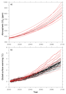
Figure 10.20. (a) 21st-century atmospheric CO2 concentration as simulated by the 11C4MIP models for the SRES A2 emission scenario (red) compared with the standard atmospheric CO2 concentration used as a forcing for many IPCC AR4 climate models (black). The standard CO2 concentration values were calculated by the BERN-CC model and are identical to those used in the TAR. For some IPCC-AR4 models, different carbon cycle models were used to convert carbon emissions to atmospheric concentrations. (b) Globally averaged surface temperature change (relative to 2000 ) simulated by theC4MIP models forced by CO2 emissions (red) compared to global warming simulated by the IPCC AR4 models forced by CO2 concentration (black). TheC4MIP global temperature change has been corrected to account for the non-CO2 radiative forcing used by the standard IPCC AR4 climate models.
Further uncertainties regarding carbon uptake were addressed with a 14-member multi-model ensemble using the CMIP2 models to quantify contributions to uncertainty from inter-model variability as opposed to internal variability ( Berthelot et al., 2002 [JoC, MoS] ). They found that the AOGCMs with the largest climate sensitivity also had the largest drying of soils in the tropics and thus the largest reduction in carbon uptake.
TheC4MIP protocol did not account for the evolution of non-CO2 greenhouse gases and aerosols. In order to compare theC4MIP simulated warming with the IPCC AR4 climate models, the SRES A2 radiative forcings of CO2 alone and total forcing (CO2 plus non-CO2 greenhouse gases and aerosols) as given in Appendix II of the TAR were used. Using these numbers and knowing the climate sensitivity of eachC4MIP model, the warming that would have been simulated by theC4MIP models if they had included the non-CO2 greenhouse gases and aerosols can be estimated. For the SRES A2 scenario, these estimates show that theC4MIP range of global temperature increase by the end of the 21st century would be 2.4°C to 5.6°C, compared with 2.6°C to 4.1°C for standard IPCC-AR4 climate models( Figure 10.20 b). As a result of a much larger CO2 concentration by 2100 in most of theC4MIP models, the upper estimate of the global warming by 2100 is up to 1.5°C higher than for the standard SRES A2 simulations.
TheC4MIP results highlight the importance of coupling the climate system and the carbon cycle in order to simulate, for a given scenario of CO2 emissions, a climate change that takes into account the dynamic evolution of the Earth’s capacity to absorb the CO2 perturbation.
Conversely, the climate-carbon cycle feedback will have an impact on the estimate of the projected CO2 emissions leading to stabilisation of atmospheric CO2 at a given level. The TAR showed the range of future emissions for the Wigley, Richels and Edmonds (WRE; Wigley et al., 1996 [PoC, JoC, SRC] ) stabilisation concentration scenarios, using different model parametrizations (including the climate-carbon feedback, Joos et al., 2001 [PoC, JoC, SRC] ; Kheshgi and Jain, 2003 [JoC, MoS] ). However, the emission reduction due to this feedback was not quantified. Similar to theC4MIP protocol, coupled and uncoupled simulations have been recently performed in order to specifically evaluate the impact of climate change on the future CO2 emissions required to achieve stabilisation ( Matthews, 2005 [JoC, SRC] ; Jones et al., 2006 [NPR, SRC] ). Figure 10.21 shows the emissions required to achieve CO2 stabilisation for the stabilisation profiles SP450, SP550, SP750 and SP 1000 (SP450 refers to stabilisation at a CO2 concentration of 450 ppm, etc.) as simulated by three climate-carbon cycle models. As detailed above, the climate-carbon cycle feedback reduces the land and ocean uptake of CO2,leading to a reduction in the emissions compatible with a given atmospheric CO2 stabilisation pathway. The higher the stabilisation scenario, the larger the climate change, the larger the impact on the carbon cycle, and hence the larger the emission reduction relative to the case without climate-carbon cycle feedback. For example, stabilising atmospheric CO2 at 450 ppm, which will likely result in a global equilibrium warming of 1.4°C to 3.1°C, with a best guess of about 2.1°C, would require a reduction of current annual greenhouse gas emissions by 52 to 90% by 2100 . Positive carbon cycle feedbacks (i.e., reduced ocean and terrestrial carbon uptake caused by the warming) reduce the total (cumulative) emissions over the 21st century compatible with a stabilisation of CO2 concentration at 450 ppm by 105 to 300 GtC relative to a hypothetical case where the carbon cycle does not respond to temperature. The uncertainty regarding the strength of the climate-carbon cycle feedback highlighted in theC4MIP analysis is also evident in Figure 10.21 .For higher stabilisation scenarios such as SP550, SP750 and SP 1000, the larger warming (2.9°C, 4.3°C and 5.5°C, respectively) requires an increasingly larger reduction (130 to 425 GtC, 160 to 500 GtC and 165 to 510 GtC, respectively) in the cumulated compatible emissions.
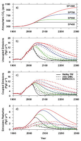
Figure 10.21. (a) Atmospheric CO2 stabilisation scenarios SP 1000 (red), SP750 (blue), SP550 (green) and SP450 (black). (b) Compatible annual emissions calculated by three models, the Hadley simple model ( Jones et al., 2006 [NPR, SRC] ; solid), the UVic EMIC ( Matthews, 2005 [JoC, SRC] ; dashed) and the BERN2.5CC EMIC ( Joos et al., 2001 [PoC, JoC, SRC] ; Plattner et al., 2001 [PoC, JoC, SRC] ; triangles) for the three stabilisation scenarios without accounting for the impact of climate on the carbon cycle (see Table 8.3 for details of the latter two models). (c) As for (b) but with the climate impact on the carbon cycle accounted for. (d) The difference between (b) and (c) showing the impact of the climate-carbon cycle feedback on the calculation of compatible emissions.
The current uncertainty involving processes driving the land and ocean carbon uptake will translate into an uncertainty in the future emissions of CO2 required to achieve stabilisation. In Figure 10.22 ,the carbon-cycle related uncertainty is addressed using the BERN2.5CC carbon cycle EMIC ( Joos et al., 2001 [PoC, JoC, SRC] ; Plattner et al., 2001 [PoC, JoC, SRC] ; see Table 8.3 for model details) and the series of S450 to SP 1000 CO2 stabilisation scenarios. The range of emission uncertainty was derived using identical assumptions as made in the TAR, varying ocean transport parameters and parametrizations describing the cycling of carbon through the terrestrial biosphere. Results are thus very closely comparable, and the small differences can be largely explained by the different CO2 trajectories and the use of a dynamic ocean model here compared to the TAR.
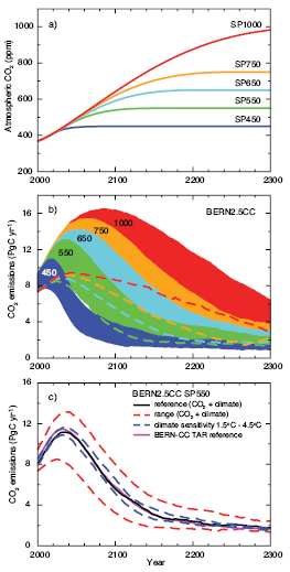
Figure 10.22. Projected CO2 emissions leading to stabilisation of atmospheric CO2 concentrations at different levels and the effect of uncertainty in carbon cycle processes on calculated emissions. Panel (a) shows the assumed trajectories of CO2 concentration (SP scenarios)(Knutti et al., 2005 ); (b) and (c) show the implied CO2 emissions, as projected with the Bern2.5CC EMIC ( Joos et al., 2001 [PoC, JoC, SRC] ; Plattner et al., 2001 [PoC, JoC, SRC] ). The ranges given in (b) for each of the SP scenarios represent effects of different model parametrizations and assumptions illustrated for scenario SP550 in panel (c) (range for ‘CO2 + climate’). The upper and lower bounds in (b) are indicated by the top and bottom of the shaded areas. Alternatively, the lower bound (where hidden) is indicated by a dashed line. Panel (c) illustrates emission ranges and sensitivities for scenario SP550.
The model results confirm that for stabilisation of atmospheric CO2,emissions need to be reduced well below year 2000 values in all scenarios. This is true for the full range of simulations covering carbon cycle uncertainty, even including the upper bound, which is based on rather extreme assumptions of terrestrial carbon cycle processes.
Cumulative emissions for the period from 2000 to 2100 (to 2300 ) range between 596 GtC (933 GtC) for SP450, and 1,236 GtC (3,052 GtC) for SP 1000 . The emission uncertainty varies between –26 and +28% about the reference cases in year 2100 and between –26 and +34% in year 2300, increasing with time. The range of uncertainty thus depends on the magnitude of the CO2 stabilisation level and the induced climate change. The additional uncertainty in projected emissions due to uncertainty in climate sensitivity is illustrated by two additional simulations with 1.5°C and 4.5°C climate sensitivities (see Box 10.2 ). The resulting emissions for this range of climate sensitivities lie within the range covered by the uncertainty in processes driving the carbon cycle.
Both the standard IPCC-AR4 and theC4MIP models ignore the effect of land cover change in future projections. However, as described in Chapters 2 and 7 ,past and future changes in land cover may affect the climate through several processes. First, they may change surface characteristics such as albedo. Second, they may affect the ratio of latent to sensible heat and therefore affect surface temperature. Third, they may induce additional CO2 emissions from the land. Fourth, they can affect the capacity of the land to take up atmospheric CO2.So far, no comprehensive coupled AOGCM has addressed these four components all together. Using AGCMs, DeFries et al. ( 2004 ) studied the impact of future land cover change on the climate, while Maynard and Royer 2004 [JoC] ) performed a similar experiment on Africa only. DeFries et al. ( 2002 ) forced the Colorado State University GCM ( Randall et al., 1996 [JoC, MoS, ARC] ) with Atmospheric Model Intercomparison Project (AMIP) climatological sea surface temperatures and with either the present-day vegetation cover or a 2050 vegetation map adapted from a low-growth scenario of the Integrated Model to Assess the Global Environment (IMAGE-2; Leemans et al., 1998 [NPR] ). The study finds that in the tropics and subtropics, replacement of forests by grassland or cropland leads to a reduction in carbon assimilation, and therefore in latent heat flux. The latter reduction leads to a surface warming of up to 1.5°C in deforested tropical regions. Using the ARPEGE-Climat AGCM ( Déqué et al., 1994 [JoC, MoS] ) with a higher resolution over Africa, Maynard et al. 2002 [JoC] ) performed two experiments, one simulation with 2 × atmospheric CO2 SSTs taken from a previous ARPEGE transient SRES B2 simulation and present-day vegetation, and one with the same SSTs but the vegetation taken from a SRES B2 simulation of the IMAGE-2 model ( Leemans et al., 1998 [NPR] ). Similar to DeFries et al. ( 2002 ), they find that future deforestation in tropical Africa leads to a redistribution of latent and sensible heat that leads to a warming of the surface. However, this warming is relatively small (0.4°C) and represents about 20% of the warming due to the atmospheric CO2 doubling.
Two recent studies further investigated the relative roles of future changes in greenhouse gases compared with future changes in land cover. Using a similar model design as Maynard and Royer 2004 [JoC] Voldoire 2006 [JoC, MoS] ) compared the climate change simulated under a 2050 SRES B2 greenhouse gases scenario to the one under a 2050 SRES B2 land cover change scenario. They show that the relative impact of vegetation change compared to greenhouse gas concentration increase is of the order of 10%, and can reach 30% over localised tropical regions. In a more comprehensive study, Feddema et al. 2005 [JoC, MoS, ARC] ) applied the same methodology for the SRES A2 and B1 scenario over the 2000 to 2100 period. Similarly, they find no significant effect at the global scale, but a potentially large effect at the regional scale, such as a warming of 2°C by 2100 over the Amazon for the A2 land cover change scenario, associated with a reduction in the DTR. The general finding of these studies is that the climate change due to land cover changes may be important relative to greenhouse gases at the regional level, where intense land cover change occurs. Globally, the impact of greenhouse gas concentrations dominates over the impact of land cover change.
10.4.2 Ocean Acidification Due to Increasing Atmospheric Carbon Dioxide
Increasing atmospheric CO2 concentrations lower oceanic pH and carbonate ion concentrations, thereby decreasing the saturation state with respect to calcium carbonate ( Feely et al., 2004 [JoC, ARC] ). The main driver of these changes is the direct geochemical effect due to the addition of anthropogenic CO2 to the surface ocean (see Box 7.3 ). Surface ocean pH today is already 0.1 unit lower than pre-industrial values( Section 5.4.2.3 ). In the multi-model median shown in Figure 10.23 ,pH is projected to decrease by another 0.3 to 0.4 units under the IS92a scenario by 2100 . This translates into a 100 to 150% increase in the concentration ofH+ ions ( Orr et al., 2005 [JoC, SRC] ). Simultaneously, carbonate ion concentrations will decrease. When water is undersaturated with respect to calcium carbonate, marine organisms can no longer form calcium carbonate shells ( Raven et al., 2005 [NPR] ).
Figure 10.23. Multi-model median for projected levels of saturation (%) with respect to aragonite, a meta-stable form of calcium carbonate, over the 21st century from the Ocean Carbon-Cycle Model Intercomparison Project (OCMIP-2) models (adapted from Orr et al., 2005 [JoC, SRC] ). Calcium carbonate dissolves at levels below 100%. Surface maps (left) and combined Pacific/Atlantic zonal mean sections (right) are given for scenario IS92a as averages over three time periods: 2011 to 2030 (top), 2045 to 2065 (middle) and 2080 to 2099 (bottom). Atmospheric CO2 concentrations for these three periods average 440, 570 and 730 ppm, respectively. Latitude-depth sections start in the North Pacific (at the left border), extend to the Southern Ocean Pacific section and return through the Southern Ocean Atlantic section to the North Atlantic (right border). At 100%, waters are saturated (solid black line - the aragonite saturation horizon); values larger than 100% indicate super-saturation; values lower than 100% indicate undersaturation. The observation-based (Global Ocean Data Analysis Project; GLODAP) 1994 saturation horizon (solid white line) is also shown to illustrate the projected changes in the saturation horizon compared to the present.
Under scenario IS92a, the multi-model projection shows large decreases in pH and carbonate ion concentrations throughout the world oceans ( Orr et al., 2005 [JoC, SRC] ; Figures 10.23 and 10.24 ). The decrease in surface carbonate ion concentrations is found to be largest at low and mid-latitudes, although undersaturation is projected to occur at high southern latitudes first( Figure 10.24 ). The present-day surface saturation state is strongly influenced by temperature and is lowest at high latitudes, with minima in the Southern Ocean. The model simulations project that undersaturation will be reached in a few decades. Therefore, conditions detrimental to high-latitude ecosystems could develop within decades, not centuries as suggested previously ( Orr et al., 2005 [JoC, SRC] ).
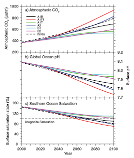
Figure 10.24. Changes in global average surface pH and saturation state with respect to aragonite in the Southern Ocean under various SRES scenarios. Time series of (a) atmospheric CO2 for the six illustrative SRES scenarios, (b) projected global average surface pH and (c) projected average saturation state in the Southern Ocean from the BERN2.5D EMIC ( Plattner et al., 2001 [PoC, JoC, SRC] ). The results for the SRES scenarios A1T and A2 are similar to those for the non-SRES scenarios S650 and IS92a, respectively. Modified from Orr et al. 2005 [JoC, SRC] ).
While the projected changes are largest at the ocean surface, the penetration of anthropogenic CO2 into the ocean interior will alter the chemical composition over the 21st century down to several thousand metres, albeit with substantial regional differences( Figure 10.23 ). The total volume of water in the ocean that is undersaturated with regard to calcite (not shown) or aragonite, a meta-stable form of calcium carbonate, increases substantially as atmospheric CO2 concentrations continue to rise( Figure 10.23 ). In the multi-model projections, the aragonite saturation horizon (i.e., the 100% line separating over- and undersaturated regions) reaches the surface in the Southern Ocean by about 2050 and substantially shoals by 2100 in the South Pacific (by >1,000 m) and throughout the Atlantic (between 800 m and 2,200 m).
Ocean acidification could thus conceivably lead to undersaturation and dissolution of calcium carbonate in parts of the surface ocean during the 21st century, depending on the evolution of atmospheric CO2 ( Orr et al., 2005 [JoC, SRC] ). Southern Ocean surface water is projected to become undersaturated with respect to aragonite at a CO2 concentration of approximately 600 ppm. This concentration threshold is largely independent of emission scenarios.
Uncertainty in these projections due to potential future climate change effects on the ocean carbon cycle (mainly through changes in temperature, ocean stratification and marine biological production and re-mineralization; see Box 7.3 )are small compared to the direct effect of rising atmospheric CO2 from anthropogenic emissions. Orr et al. 2005 [JoC, SRC] ) estimate that 21st century climate change could possibly counteract less than 10% of the projected direct geochemical changes. By far the largest uncertainty in the future evolution of these ocean interior changes is thus associated with the future pathway of atmospheric CO2.
10.4.3 Simulations of Future Evolution of Methane, Ozone and Oxidants
Simulations using coupled chemistry-climate models indicate that the trend in upper-stratospheric ozone changes sign sometime between 2000 and 2005 due to the gradual reduction in halocarbons. While ozone concentrations in the upper stratosphere decreased at a rate of 400 ppb (–6%) per decade during 1980 to 2000, they are projected to increase at a rate of 100 ppb (1 to 2%) per decade from 2000 to 2020 ( Austin and Butchart, 2003 [JoC, MoS, ARC] ). On longer time scales, simulations show significant changes in ozone and CH4 relative to current concentrations. The changes are related to a variety of factors, including increased emissions of chemical precursors, changes in gas-phase and heterogeneous chemistry, altered climate conditions due to global warming and greater transport and mixing across the tropopause. The impacts on CH4 and ozone from increased emissions are a direct effect of anthropogenic activity, while the impacts of different climate conditions and stratosphere-troposphere exchange represent indirect effects of these emissions ( Grewe et al., 2001 [JoC, MoS] ).
The projections for ozone based upon scenarios with high emissions (IS92a; Leggett et al., 1992 [NPR] ) and SRES A2 ( Nakićenović and Swart, 2000 [NPR] ) indicate that concentrations of tropospheric ozone might increase throughout the 21st century, primarily as a result of these emissions. Simulations for the period 2015 through 2050 project increases in ozone of 20 to 25% ( Grewe et al., 2001 [JoC, MoS] ; Hauglustaine and Brasseur, 2001 [JoC, MoS, ARC] ), and simulations through 2100 indicate that ozone below 250 mb may grow by 40 to 60% ( Stevenson et al., 2000 [JoC, MoS, ARC] ;( Grenfell et al., 2003; ) Zeng and Pyle, 2003 [JoC, MoS] ; Hauglustaine et al., 2005 [JoC, MoS, ARC] ; Yoshimura et al., 2006 [SRC] ). The primary species contributing to the increase in tropospheric ozone are anthropogenic emissions of NOx,CH4,CO and compounds from fossil fuel combustion. The photochemical reactions that produce smog are accelerated by increases of 2.6 times the present flux of NOx,2.5 times the present flux of CH4 and 1.8 times the present flux of CO in the A2 scenario. Between 91 and 92% of the higher concentrations in ozone are related to direct effects of these emissions, with the remainder of the increase attributable to secondary effects of climate change ( Zeng and Pyle, 2003 [JoC, MoS] ) combined with biogenic precursor emissions ( Hauglustaine et al., 2005 [JoC, MoS, ARC] ). These emissions may also lead to higher concentrations of oxidants including the hydroxyl radical (OH), possibly leading to an 8% reduction in the lifetime of tropospheric CH4 ( Grewe et al., 2001 [JoC, MoS] ).
Since the projected growth in emissions occurs primarily in low latitudes, the ozone increases are largest in the tropics and subtropics ( (Grenfell et al., 2003 ) ). In particular, the concentrations in Southeast Asia, India and Central America increase by 60 to 80% by 2050 under the A2 scenario. However, the effects of tropical emissions are not highly localised, since the ozone spreads throughout the lower atmosphere in plumes emanating from these regions. As a result, the ozone in remote marine regions in the SH may grow by 10 to 20% over present-day levels by 2050 . The ozone may also be distributed through vertical transport in tropical convection followed by lateral transport on isentropic surfaces. Ozone concentrations can also be increased by emissions of biogenic hydrocarbons (e.g., Hauglustaine et al., 2005 [JoC, MoS, ARC] ), in particular isoprene emitted by broadleaf forests. Under the A2 scenario, biogenic hydrocarbons are projected to increase by between 27% ( Sanderson et al., 2003 [JoC] ) and 59% ( Hauglustaine et al., 2005 [JoC, MoS, ARC] ) contributing to a 30 to 50% increase in ozone formation over northern continental regions.
Developing countries have begun reducing emissions from mobile sources through stricter standards. New projections of the evolution of ozone precursors that account for these reductions have been developed with the Regional Air Pollution Information and Simulation (RAINS) model ( Amann et al., 2004 [NPR, MoS] ). One set of projections is consistent with source strengths permitted under the Current Legislation (CLE) scenario. A second set of projections is consistent with lower emissions under a Maximum Feasible Reduction (MFR) scenario. The concentrations of ozone and CH4 have been simulated for the MFR, CLE and A2 scenarios for the period 2000 through 2030 using an ensemble of 26 chemical transport models ( Dentener et al., 2006 [ARC] ; Stevenson et al., 2006 [JoC, MoS, ARC] ). The changes in NOx emissions for these three scenarios are –27%, +12% and +55%, respectively, relative to year 2000 . The corresponding changes in ensemble-mean burdens in tropospheric ozone are –5%, +6% and +18% for the MFR, CLE and A2 scenarios, respectively. There are substantial inter-model differences of order ±25% in these results. The ozone decreases throughout the troposphere in the MFR scenario, but the zonal annual mean concentrations increase by up to 6 ppb in the CLE scenario and by typically 6 to 10 ppb in the A2 scenario (Supplementary Material, Figure S10.2).
The radiative forcing by the combination of ozone and CH4 changes by –0.05, 0.18, and 0.30 Wm–2 for the MFR, CLE and A2 scenarios, respectively. These projections indicate that the growth in tropospheric ozone between 2000 and 2030 could be reduced or reversed depending on emission controls.
The major issues in the fidelity of these simulations for future tropospheric ozone are the sensitivities to the representation of the stratospheric production, destruction and transport of ozone and the exchange of species between the stratosphere and troposphere. Few of the models include the effects of non-methane hydrocarbons (NMHCs), and the sign of the effects of NMHCs on ozone are not consistent among the models that do ( Hauglustaine and Brasseur, 2001 [JoC, MoS, ARC] ;( Grenfell et al., 2003 ) ).
The effect of more stratosphere-troposphere exchange (STE) in response to climate change is projected to increase the concentrations of ozone in the upper troposphere due to the much greater concentrations of ozone in the lower stratosphere than in the upper troposphere. While the sign of the effect is consistent in recent simulations, the magnitude of the change in STE and its effects on ozone are very model dependent. In a simulation forced by the SRES A1FI scenario, Collins et al. 2003 [JoC, MoS] ) project that the downward flux of ozone increases by 37% from the 1990 s to the 2090 s. As a result, the concentration of ozone in the upper troposphere at mid-latitudes increases by 5 to 15%. For the A2 scenarios, projections of the increase in ozone by 2100 due to STE range from 35% ( Hauglustaine et al., 2005 [JoC, MoS, ARC] ) to 80% ( Sudo et al., 2003 [JoC, MoS, ARC] ; Zeng and Pyle, 2003 [JoC, MoS] ). The increase in STE is driven by increases in the descending branches of the Brewer-Dobson Circulation at mid-latitudes and is caused by changes in meridional temperature gradients in the upper troposphere and lower stratosphere ( Rind et al., 2001 [JoC, ARC] ). The effects of the enhanced STE are sensitive to the simulation of processes in the stratosphere, including the effects of lower temperatures and the evolution of chlorine, bromine and NOx concentrations. Since the greenhouse effect of ozone is largest in the upper troposphere, the treatment of STE remains a significant source of uncertainty in the calculation of the total greenhouse effect of tropospheric ozone.
The effects of climate change, in particular increased tropospheric temperatures and water vapour, tend to offset some of the increase in ozone driven by emissions. The higher water vapour is projected to offset the increase in ozone by between 10% ( Hauglustaine et al., 2005 [JoC, MoS, ARC] ) and 17% ( Stevenson et al., 2000 [JoC, MoS, ARC] ). The water vapour both decelerates the chemical production and accelerates the chemical destruction of ozone. The photochemical production depends on the concentrations of NOy (reactive odd nitrogen), and the additional water vapour causes a larger fraction of NOy to be converted to nitric acid, which can be efficiently removed from the atmosphere in precipitation ( Grewe et al., 2001 [JoC, MoS] ). The water vapour also increases the concentrations of OH through reaction with the oxygen radical in the 1D excited state (O(1D)), and the removal of O(1D) from the atmosphere slows the formation of ozone. The increased concentrations of OH and the increased rates of CH4 oxidation with higher temperature further reduce the lifetime of tropospheric CH4 by 12% by 2100 ( Stevenson et al., 2000 [JoC, MoS, ARC] ; Johnson et al., 2001 [JoC, MoS, ARC] ). Decreases in CH4 concentrations also tend to reduce tropospheric ozone ( Stevenson et al., 2000 [JoC, MoS, ARC] ).
Recent measurements show that CH4 growth rates have declined and were negative for several years in the early 21st century (see Section 2.3.2 ). The observed rate of increase of 0.8 ppb yr–1 for the period 1999 to 2004 is considerably less than the rate of 6 ppb yr–1 assumed in all the SRES scenarios for the period 1990 to 2000 ( Nakićenović and Swart, 2000 [NPR] ; TAR Appendix II). Recent studies ( Dentener et al., 2005 [MoS, ARC] ) have considered lower emission scenarios (see above) that take account of new pollution control techniques adopted in major developing countries. In the CLE scenario, emissions of CH4 are comparable to the B2 scenario and increase from 340 Tg yr–1 in 2000 to 450 Tg yr–1 in 2030 . The CH4 concentrations increase from 1,750 ppb in 2000 to between 2,090 and 2,200 ppb in 2030 under this scenario. In the MFR scenario, the emissions are sufficiently low that the concentrations in 2030 are unchanged at 1,750 ppb. Under these conditions, the changes in radiative forcing due to CH4 between the 1990 s and 2020 s are less than 0.01 Wm–2.
Current understanding of the magnitude and variation of CH4 sources and sinks is covered in Section 7.4 ,where it is noted that there are substantial uncertainties although the modelling has progressed. There is some evidence for a coupling between climate and wetland emissions. For example, calculations using atmospheric concentrations and small-scale emission measurements as input differ by 60% ( Shindell and Schmidt, 2004 [PoC, JoC, SRC] ). Concurrent changes in natural sources of CH4 are now being estimated to first order using simple models of the biosphere coupled to AOGCMs. Simulations of the response of wetlands to climate change from doubling atmospheric CO2 show that wetland emissions increase by 78% ( Shindell and Schmidt, 2004 [PoC, JoC, SRC] ). Most of this effect is caused by growth in the flux of CH4 from existing tropical wetlands. The increase would be equivalent to approximately 20% of current inventories and would contribute an additional 430 ppb to atmospheric concentrations. Global radiative forcing would increase by approximately 4 to 5% from the effects of wetland emissions by 2100 ( Gedney et al., 2004 [JoC, ARC] ).
10.4.4 Simulations of Future Evolution of Major Aerosol Species
The time-dependent evolution of major aerosol species and the interaction of these species with climate represent some of the major sources of uncertainty in projections of climate change. An increasing number of AOGCMs have included multiple types of tropospheric aerosols including sulphates, nitrates, black and organic carbon, sea salt and soil dust. Of the 23 models represented in the multi-model ensemble of climate-change simulations for IPCC AR4, 13 include other tropospheric species besides sulphates. Of these, seven have the non-sulphate species represented with parametrizations that interact with the remainder of the model physics. Nitrates are treated in just two of the models in the ensemble. Recent projections of nitrate and sulphate loading under the SRES A2 scenario suggest that forcing by nitrates may exceed forcing by sulphates by the end of the 21st century ( Adams et al., 2001 [JoC, MoS] ). This result is of course strongly dependent upon the evolution of precursor emissions for these aerosol species.
The black and organic carbon aerosols in the atmosphere include a very complex system of primary organic aerosols (POA) and secondary organic aerosols (SOA), which are formed by oxidation of biogenic VOCs. The models used for climate projections typically use highly simplified bulk parametrizations for POA and SOA. More detailed parametrizations for the formation of SOA that trace oxidation pathways have only recently been developed and used to estimate the direct radiative forcing by SOA for present-day conditions ( Chung and Seinfeld, 2002 [JoC, MoS] ). The forcing by SOA is an emerging issue for simulations of present-day and future climate since the rate of chemical formation of SOA may be 60% or more of the emissions rate for primary carbonaceous aerosols ( Kanakidou et al., 2005 [MoS] ). In addition, two-way coupling between reactive chemistry and tropospheric aerosols has not been explored comprehensively in climate change simulations. Unified models that treat tropospheric ozone-NOx-hydrocarbon chemistry, aerosol formation, heterogeneous processes in clouds and on aerosols, and gas-phase photolysis have been developed and applied to the current climate ( Liao et al., 2003 [JoC, MoS] ). However, these unified models have not yet been used extensively to study the evolution of the chemical state of the atmosphere under future scenarios.
The interaction of soil dust with climate is under active investigation. Whether emissions of soil dust aerosols increase or decrease in response to changes in atmospheric state and circulation is still unresolved ( Tegen et al., 2004a [JoC, MoS] ). Several recent studies have suggested that the total surface area where dust can be mobilised will decrease in a warmer climate with higher concentrations of CO2 (e.g., Harrison et al., 2001 [MoS] ). The net effects of reductions in dust emissions from natural sources combined with land use change could potentially be significant but have not been systematically modelled as part of climate change assessment.
Uncertainty regarding the scenario simulations is compounded by inherently unpredictable natural forcings from future volcanic eruptions and solar variability. The eruptions that produce climatologically significant forcing represent just the extremes of global volcanic activity ( Naveau and Ammann, 2005 [PoC, JoC, ARC] ). Global simulations can account for the effects of future natural forcings using stochastic representations based upon prior eruptions and variations in solar luminosity. The relative contribution of these forcings to the projections of global mean temperature anomalies are largest in the period up to 2030 ( Stott and Kettleborough, 2002 [JoC, MoS, SRC] ).
10.5 Quantifying the Range of Climate Change Projections
10.5.1 Sources of Uncertainty and Hierarchy of Models
Uncertainty in predictions of anthropogenic climate change arises at all stages of the modelling process described in Section 10.1 .The specification of future emissions of greenhouse gases, aerosols and their precursors is uncertain (e.g., Nakićenović and Swart, 2000 [NPR] ). It is then necessary to convert these emissions into concentrations of radiatively active species, calculate the associated forcing and predict the response of climate system variables such as surface temperature and precipitation( Figure 10.1 ). At each step, uncertainty in the true signal of climate change is introduced both by errors in the representation of Earth system processes in models (e.g., Palmer et al., 2005 [Ambiguous] ) and by internal climate variability (e.g., Selten et al., 2004 [JoC, MoS] ). The effects of internal variability can be quantified by running models many times from different initial conditions, provided that simulated variability is consistent with observations. The effects of uncertainty in the knowledge of Earth system processes can be partially quantified by constructing ensembles of models that sample different parametrizations of these processes. However, some processes may be missing from the set of available models, and alternative parametrizations of other processes may share common systematic biases. Such limitations imply that distributions of future climate responses from ensemble simulations are themselves subject to uncertainty ( Smith, 2002 [JoC, MoS] ), and would be wider were uncertainty due to structural model errors accounted for. These distributions may be modified to reflect observational constraints expressed through metrics of the agreement between the observed historical climate and the simulations of individual ensemble members, for example through Bayesian methods (see Chapter9 Supplementary Material, Appendix 9.B ). In this case, the choice of observations and their associated errors introduce further sources of uncertainty. In addition, some sources of future radiative forcing are yet to be accounted for in the ensemble projections, including those from land use change, variations in solar and volcanic activity ( Kettleborough et al., 2007 [JoC, MoS, SRC, 2007] ), and CH4 release from permafrost or ocean hydrates (see Section 8.7 ).
Aspectrum or hierarchy of models of varying complexity has been developed ( Claussen et al., 2002 [JoC, MoS, ARC] ; Stocker and Knutti, 2003 [MoS, SRC] ) to assess the range of future changes consistent with the understanding of known uncertainties. Simple climate models (SCMs) typically represent the ocean-atmosphere system as a set of global or hemispheric boxes, predicting global surface temperature using an energy balance equation, a prescribed value of climate sensitivity and a basic representation of ocean heat uptake (see Section 8.8.2 ). Their role is to perform comprehensive analyses of the interactions between global variables, based on prior estimates of uncertainty in their controlling parameters obtained from observations, expert judgement and from tuning to complex models. By coupling SCMs to simple models of biogeochemical cycles they can be used to extrapolate the results of AOGCM simulations to a wide range of alternative forcing scenarios (e.g., Wigley and Raper, 2001 [PoC, JoC, MoS, SRC] ; see Section 10.5.3 ).
Compared to SCMs, EMICs include more of the processes simulated in AOGCMs, but in a less detailed, more highly parametrized form (see Section 8.8.3 ), and at coarser resolution. Consequently, EMICs are not suitable for quantifying uncertainties in regional climate change or extreme events, however they can be used to investigate the large-scale effects of coupling between multiple Earth system components in large ensembles or long simulations (e.g., Forest et al., 2002 [JoC, ARC] ; Knutti et al., 2002 [Ambiguous] ), which is not yet possible with AOGCMs due to their greater computational expense. Some EMICs therefore include modules such as vegetation dynamics, the terrestrial and ocean carbon cycles and atmospheric chemistry ( Plattner et al., 2001 [PoC, JoC, SRC] ; Claussen et al., 2002 [JoC, MoS, ARC] ), filling a gap in the spectrum of models between AOGCMs and SCMs. Thorough sampling of parameter space is computationally feasible for some EMICs (e.g., Stocker and Schmittner, 1997 [JoC, SRC] ; Forest et al., 2002 [JoC, ARC] ; Knutti et al., 2002 [Ambiguous] ), as for SCMs ( Wigley and Raper, 2001 [PoC, JoC, MoS, SRC] ), and is used to obtain probabilistic projections (see Section 10.5.4.5 ). In some EMICs, climate sensitivity is an adjustable parameter, as in SCMs. In other EMICs, climate sensitivity is dependent on multiple model parameters, as in AOGCMs. Probabilistic estimates of climate sensitivity and TCR from SCMs and EMICs are assessed in Section 9.6 and compared with estimates from AOGCMs in Box 10.2 .
The high resolution and detailed parametrizations in AOGCMs enable them to simulate more comprehensively the processes giving rise to internal variability (see Section 8.4 ), extreme events (see Section 8.5 )and climate change feedbacks, particularly at the regional scale ( Boer and Yu, 2003a [JoC] ; Bony and Dufresne, 2005 [JoC, MoS, ARC] ; Bony et al., 2006 [JoC, ARC] ; Soden and Held, 2006 [JoC, MoS, ARC] ). Given that ocean dynamics influence regional feedbacks ( Boer and Yu, 2003b [JoC] ), quantification of regional uncertainties in time-dependent climate change requires multi-model ensemble simulations with AOGCMs containing a full, three-dimensional dynamic ocean component. However, downscaling methods (see Chapter 11 )are required to obtain credible information at spatial scales near or below the AOGCM grid scale (125 to 400 km in the AR4 AOGCMs, see Table 8.1 ).
Box 10.2: Equilibrium Climate Sensitivity
The likely range [1] for equilibrium climate sensitivity was estimated in the TAR (Technical Summary, Section F.3; Cubasch et al., 2001 [NPR, MoS, ARC] ) to be 1.5°C to 4.5°C. The range was the same as in an early report of the National Research Council ( Charney, 1979 [NPR] ), and the two previous IPCC assessment reports ( Mitchell et al., 1990 [NPR, MoS] ; Kattenberg et al., 1996 [NPR, MoS] ). These estimates were expert assessments largely based on equilibrium climate sensitivities simulated by atmospheric GCMs coupled to non-dynamic slab oceans. The mean ±1 standard deviation values from these models were 3.8°C ± 0.78°C in the SAR (17 models), 3.5°C ± 0.92°C in the TAR (15 models) and in this assessment 3.26°C ± 0.69°C (18 models).
Considerable work has been done since the TAR ( IPCC, 2001 [NPR] ) to estimate climate sensitivity and to provide a better quantification of relative probabilities, including a most likely value, rather than just a subjective range of uncertainty. Since climate sensitivity of the real climate system cannot be measured directly, new methods have been used since the TAR to establish a relationship between sensitivity and some observable quantity (either directly or through a model), and to estimate a range or probability density function (PDF) of climate sensitivity consistent with observations. These methods are summarised separately in Chapters 9 and 10 ,and here we synthesize that information into an assessment. The information comes from two main categories: constraints from past climate change on various time scales, and the spread of results for climate sensitivity from ensembles of models.
The first category of methods (see Section 9.6 )uses the historical transient evolution of surface temperature, upper air temperature, ocean temperature, estimates of the radiative forcing, satellite data, proxy data over the last millennium, or a subset thereof to calculate ranges or PDFs for sensitivity (e.g., Wigley et al., 1997b [NPR, PoC, SRC] ; Tol and de Vos, 1998 [JoC] ; Andronova and Schlesinger, 2001 [JoC, MoS, ARC] ; Forest et al., 2002 [JoC, ARC] ; Gregory et al., 2002a [JoC, MoS, SRC] ; Harvey and Kaufmann, 2002 [JoC, MoS] ; Knutti et al., 2002 [Ambiguous] , 2003; Frame et al., 2005 [JoC, MoS] ; Forest et al., 2006 [JoC, MoS, SRC] ; Forster and Gregory, 2006 [JoC, SRC] ; Hegerl et al., 2006 [PoC, JoC, SRC] ). A summary of all PDFs of climate sensitivity from those methods is shown in Figure 9.20 and in Box 10.2, Figure 1a. Median values, most likely values (modes) and 5 to 95% uncertainty ranges are shown in Box 10.2, Figure 1b for each PDF. Most of the results confirm that climate sensitivity is very unlikely below 1.5°C. The upper bound is more difficult to constrain because of a nonlinear relationship between climate sensitivity and the observed transient response, and is further hampered by the limited length of the observational record and uncertainties in the observations, which are particularly large for ocean heat uptake and for the magnitude of the aerosol radiative forcing. Studies that take all the important known uncertainties in observed historical trends into account cannot rule out the possibility that the climate sensitivity exceeds 4.5°C, although such high values are consistently found to be less likely than values of around 2.0°C to 3.5°C. Observations of transient climate change provide better constraints for the TCR (see Section 9.6.1.3).
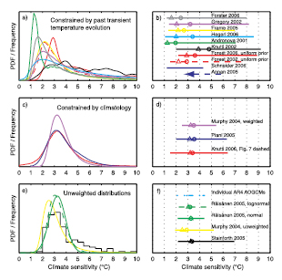
Box 10.2, Figure 1. (a) PDFs or frequency distributions constrained by the transient evolution of the atmospheric temperature, radiative forcing and ocean heat uptake, (b) as in (a) and (b) but 5 to 95% ranges, medians (circles) and maximum probabilities (triangles), (c) and (d) as in (a) but using constraints from present-day climatology, and (e) and (f) unweighted or fitted distributions from different models or from perturbing parameters in a single model. Distributions in (e) and (f) should not be strictly interpreted as PDFs. See Chapter9 text, Figure 9.20 and Table 9.3 for details. Note that Annan et al. 2005b [MoS, SRC] ) only provide an upper but no lower bound. All PDFs are truncated at 10°C for consistency, some are shown for different prior distributions than in the original studies, and ranges may differ from numbers reported in individual studies.
Two recent studies use a modelled relation between climate sensitivity and tropical SSTs in the Last Glacial Maximum (LGM) and proxy records of the latter to estimate ranges of climate sensitivity ( Annan et al., 2005b [MoS, SRC] ; Schneider von Deimling et al., 2006 [PoC, JoC, MoS, ARC] ; see Section 9.6 ). While both of these estimates overlap with results from the instrumental period and results from other AOGCMS, the results differ substantially due to different forcings and the different relationships between LGM SSTs and sensitivity in the models used. Therefore, LGM proxy data provide support for the range of climate sensitivity based on other lines of evidence.
Studies comparing the observed transient response of surface temperature after large volcanic eruptions with results obtained from models with different climate sensitivities (see Section. 9.6) do not provide PDFs, but find best agreement with sensitivities around 3°C, and reasonable agreement within the 1.5°C to 4.5°C range ( Wigley et al., 2005 [PoC, JoC, SRC] ). They are not able to exclude sensitivities above 4.5°C.
The second category of methods examines climate sensitivity in GCMs. Climate sensitivity is not a single tuneable parameter in these models, but depends on many processes and feedbacks. Three PDFs of climate sensitivity were obtained by comparing different variables of the simulated present-day climatology and variability against observations in a perturbed physics ensemble ( Murphy et al., 2004 [JoC, MoS, SRC] ; Piani et al., 2005 [JoC, MoS, SRC] ; Knutti et al., 2006 [JoC, SRC] , Box 10.2, Figure 1c,d; see Section 10.5.4.2 ). Equilibrium climate sensitivity is found to be most likely around 3.2°C, and very unlikely to be below about 2°C. The upper bound is sensitive to how model parameters are sampled and to the method used to compare with observations.
Box 10.2, Figure 1e,f show the frequency distributions obtained by different methods when perturbing parameters in the Hadley Centre Atmospheric Model (HadAM3) but before weighting with observations (Section10.5.4). Murphy et al. 2004 [JoC, MoS, SRC] ; unweighted) sampled 29 parameters and assumed individual effects to combine linearly. Stainforth et al. 2005 [JoC, MoS, SRC] ) found nonlinearities when simulating multiple combinations of a subset of key parameters. The most frequently occurring climate sensitivity values are grouped around 3°C, but this could reflect the sensitivity of the unperturbed model. Some, but not all, of the simulations by high-sensitivity models have been found to agree poorly with observations and are therefore unlikely, hence even very high values are not excluded. This inability to rule out very high values is common to many methods, since for well-understood physical reasons, the rate of change (against sensitivity) of most quantities that can be observed tends to zero as the sensitivity increases ( Hansen et al., 1985 [JoC, SRC] ; Knutti et al., 2005 [JoC, MoS, SRC] ; Allen et al., 2006b [NPR, SRC] ).
There is no well-established formal way of estimating a single PDF from the individual results, taking account of the different assumptions in each study. Most studies do not account for structural uncertainty, and thus probably tend to underestimate the uncertainty. On the other hand, since several largely independent lines of evidence indicate similar most likely values and ranges, climate sensitivity values are likely to be better constrained than those found by methods based on single data sets ( Annan and Hargreaves, 2006 [JoC, MoS, SRC] ; Hegerl et al., 2006 [PoC, JoC, SRC] ).
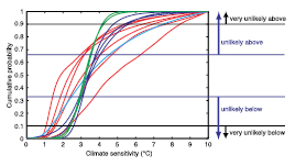
Box 10.2, Figure 2. Individual cumulative distributions of climate sensitivity from the observed 20th-century warming (red), model climatology (blue) and proxy evidence (cyan), taken from Box 10.2, Figure 1a, c (except LGM studies and Forest et al. 2002 [JoC, ARC] ), which is superseded by Forest et al. 2006 [JoC, MoS, SRC] )) and cumulative distributions fitted to the AOGCMs’ climate sensitivities (green) from Box 10.2, Figure 1e. Horizontal lines and arrows mark the edges of the likelihood estimates according to IPCC guidelines.
The equilibrium climate sensitivity values for the AR4 AOGCMs coupled to non-dynamic slab ocean models are given for comparison (Box 10.2, Figure 1e,f; see also Table 8.2 ). These estimates come from models that represent the current best efforts from the international global climate modelling community at simulating climate. A normal fit yields a 5 to 95% range of about 2.1°C to 4.4°C with a mean value of equilibrium climate sensitivity of about 3.3°C (2.2°C to 4.6°C for a lognormal distribution, median 3.2°C) ( Räisänen, 2005b [MoS, SRC] ). A probabilistic interpretation of the results is problematic, because each model is assumed to be equally credible and the results depend upon the assumed shape of the fitted distribution. Although the AOGCMs used in IPCC reports are an ‘ensemble of opportunity’ not designed to sample modelling uncertainties systematically or randomly, the range of sensitivities covered has been rather stable over many years. This occurs in spite of substantial model developments, considerable progress in simulating many aspects of the large-scale climate, and evaluation of those models against observations. Progress has been made since the TAR in diagnosing and understanding inter-model differences in climate feedbacks and equilibrium climate sensitivity. Confidence has increased in the strength of water vapour-lapse rate feedbacks, whereas cloud feedbacks (particularly from low-level clouds) have been confirmed as the primary source of climate sensitivity differences (see Section 8.6 ).
Since the TAR, the levels of scientific understanding and confidence in quantitative estimates of equilibrium climate sensitivity have increased substantially. Basing our assessment on a combination of several independent lines of evidence, as summarised in Box 10.2 Figures 1 and 2, including observed climate change and the strength of known feedbacks simulated in GCMs, we conclude that the global mean equilibrium warming for doubling CO2,or ‘equilibrium climate sensitivity’, is likely to lie in the range 2°C to 4.5°C, with a most likely value of about 3°C. Equilibrium climate sensitivity is very likely larger than 1.5°C.
For fundamental physical reasons as well as data limitations, values substantially higher than 4.5°C still cannot be excluded, but agreement with observations and proxy data is generally worse for those high values than for values in the 2°C to 4.5°C range.
10.5.2 Range of Responses from Different Models
10.5.2.1 Comprehensive AOGCMs
The way a climate model responds to changes in external forcing, such as an increase in anthropogenic greenhouse gases, is characterised by two standard measures: (1) ‘equilibrium climate sensitivity’ (the equilibrium change in global surface temperature following a doubling of the atmospheric equivalent CO2 concentration; see Glossary), and (2) ‘transient climate response’ (the change in global surface temperature in a global coupled climate model in a 1% yr–1 CO2 increase experiment at the time of atmospheric CO2 doubling; see Glossary). The first measure provides an indication of feedbacks mainly residing in the atmospheric model but also in the land surface and sea ice components, and the latter quantifies the response of the fully coupled climate system including aspects of transient ocean heat uptake (e.g., Sokolov et al., 2003 [JoC, SRC] ). These two measures have become standard for quantifying how an AOGCM will react to more complicated forcings in scenario simulations.
Historically, the equilibrium climate sensitivity has been given in the range from 1.5°C to 4.5°C. This range was reported in the TAR with no indication of a probability distribution within this range. However, considerable recent work has addressed the range of equilibrium climate sensitivity, and attempted to assign probabilities to climate sensitivity.
Equilibrium climate sensitivity and TCR are not independent( Figure 10.25 a). For a given AOGCM, the TCR is smaller than the equilibrium climate sensitivity because ocean heat uptake delays the atmospheric warming. A large ensemble of the BERN2.5D EMIC has been used to explore the relationship of TCR and equilibrium sensitivity over a wide range of ocean heat uptake parametrizations ( Knutti et al., 2005 [JoC, MoS, SRC] ). Good agreement with the available results from AOGCMs is found, and the BERN2.5D EMIC covers almost the entire range of structurally different models. The percent change in precipitation is closely related to the equilibrium climate sensitivity for the current generation of AOGCMs( Figure 10.25 b), with values from the current models falling within the range of the models from the TAR. Figure 10.25 cshows the percent change in globally averaged precipitation as a function of TCR at the time of atmospheric CO2 doubling, as simulated by 1% yr–1 transient CO2 increase experiments with AOGCMs. The figure suggests a broadly positive correlation between these two quantities similar to that for equilibrium climate sensitivity, with these values from the new models also falling within the range of the previous generation of AOGCMs assessed in the TAR. Note that the apparent relationships may not hold for other forcings or at smaller scales. Values for an ensemble with perturbations made to parameters in the atmospheric component of UKMO-HadCM3 (M. Collins et al., 2006 [Ambiguous] ) cover similar ranges and are shown in Figure 10.25 for comparison.
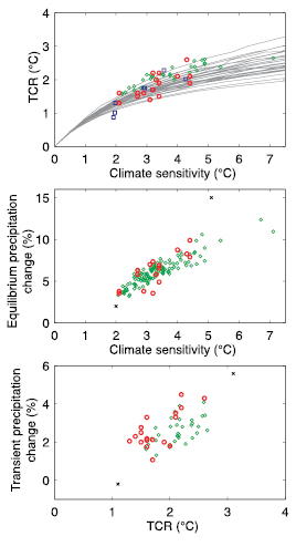
Figure 10.25. (a) TCR versus equilibrium climate sensitivity for all AOGCMs (red), EMICs (blue), a perturbed physics ensemble of the UKMO-HadCM3 AOGCM (green; an updated ensemble based on M. Collins et al., 2006 [Ambiguous] ) and from a large ensemble of the Bern2.5D EMIC ( Knutti et al., 2005 [JoC, MoS, SRC] ) using different ocean vertical diffusivities and mixing parametrizations (grey lines). (b) Global mean precipitation change (%) as a function of global mean temperature change at equilibrium for doubled CO2 in atmospheric GCMs coupled to a non-dynamic slab ocean (red all AOGCMS, green from a perturbed physics ensemble of the atmosphere-slab ocean version of UKMO-HadCM3 ( Webb et al., 2006 [JoC, ARC] )). (c) Global mean precipitation change (%) as a function of global mean temperature change (TCR) at the time of CO2 doubling in a transient 1% yr–1 CO2 increase scenario, simulated by coupled AOGCMs (red) and the UKMO-HadCM3 perturbed physics ensemble (green). Black crosses in (b) and (c) mark ranges covered by the TAR AOGCMs ( IPCC, 2001 [NPR] ) for each quantity.
Fitting normal distributions to the results, the 5 to 95% uncertainty range for equilibrium climate sensitivity from the AOGCMs is approximately 2.1°C to 4.4°C and that for TCR is 1.2°C to 2.4°C (using the method of Räisänen, 2005b [MoS, SRC] ). The mean for climate sensitivity is 3.26°C and that for TCR is 1.76°C. These numbers are practically the same for both the normal and the lognormal distribution (see Box 10.2 ). The assumption of a (log) normal fit is not well supported by the limited sample of AOGCM data. In addition, the AOGCMs represent an ‘ensemble of opportunity’ and are by design not sampled in a random way. However, most studies aiming to constrain climate sensitivity with observations do indeed indicate a similar to lognormal probability distribution of climate sensitivity and an approximately normal distribution of the uncertainty in future warming and thus TCR (see Box 10.2 ). Those studies also suggest that the current AOGCMs may not cover the full range of uncertainty for climate sensitivity. An assessment of all the evidence on equilibrium climate sensitivity is provided in Box 10.2 .The spread of the AOGCM climate sensitivities is discussed in Section 8.6 and the AOGCM values for climate sensitivity and TCR are listed in Table 8.2 .
The nonlinear relationship between TCR and equilibrium climate sensitivity shown in Figure 10.25 aalso indicates that on time scales well short of equilibrium, the model’s TCR is not particularly sensitive to the model’s climate sensitivity. The implication is that transient climate change is better constrained than the equilibrium climate sensitivity, that is, models with different sensitivity might still show good agreement for projections on decadal time scales. Therefore, in the absence of unusual solar or volcanic activity, climate change is well constrained for the coming few decades, because differences in some feedbacks will only become important on long time scales (see also Section 10.5.4.5 )and because over the next few decades, about half of the projected warming would occur as a result of radiative forcing being held constant at year 2000 levels (constant composition commitment, see Section 10.7 ).
Comparing observed thermal expansion with those AR4 20th-century simulations that have natural forcings indicates that ocean heat uptake in the models may be 25% larger than observed, although both could be consistent within their uncertainties. This difference is possibly due to a combination of overestimated ocean heat uptake in the models, observational uncertainties and limited data coverage in the deep ocean (see Sections 9.5.1.1 , 9.5.2 ,and 9.6.2.1 ). Assigning this difference solely to overestimated ocean heat uptake, the TCR estimates could increase by 0.6°C at most. This is in line with evidence for a relatively weak dependence of TCR on ocean mixing based on SCMs and EMICS ( Allen et al., 2000 [JoC, MoS, SRC] ; Knutti et al., 2005 [JoC, MoS, SRC] ). The range of TCR covered by an ensemble with perturbations made to parameters in the atmospheric component of UKMO-HadCM3 is 1.5 to 2.6°C (M. Collins et al., 2006 [Ambiguous] ), similar to the AR4 AOGCM range. Therefore, based on the range covered by AOGCMs, and taking into account structural uncertainties and possible biases in transient heat uptake, TCR is assessed as very likely larger than 1°C and very unlikely greater than 3°C (i.e., 1.0°C to 3.0°C is a 10 to 90% range). Because the dependence of TCR on sensitivity becomes small as sensitivity increases, uncertainties in the upper bound on sensitivity only weakly affect the range of TCR (see Figure 10.25 ; Chapter9 ;Knutti et al., 2005 [JoC, MoS, SRC] ; Allen et al., 2006b [NPR, SRC] ). Observational constraints based on detection and attribution studies provide further support for this TCR range (see Section 9.6.2.3 ).
10.5.2.2 Earth System Models of Intermediate Complexity
Over the last few years, a range of climate models has been developed that are dynamically simpler and of lower resolution than comprehensive AOGCMs, although they might well be more ‘complete’ in terms of climate system components that are included. The class of such models, usually referred to as EMICs ( Claussen et al., 2002 [JoC, MoS, ARC] ), is very heterogeneous, ranging from zonally averaged ocean models coupled to energy balance models ( Stocker et al., 1992a [JoC, MoS, SRC] ) or to statistical-dynamical models of the atmosphere ( Petoukhov et al., 2000 [JoC, MoS, ARC] ), to low resolution three-dimensional ocean models, coupled to energy balance or simple dynamical models of the atmosphere ( Opsteegh et al., 1998 [JoC, MoS] ; Edwards and Marsh, 2005 [JoC, MoS, SRC] ; Müller et al., 2006 [PoC, JoC, MoS, SRC] ). Some EMICs have a radiation code and prescribe greenhouse gases, while others use simplified equations to project radiative forcing from projected concentrations and abundances ( Joos et al., 2001 [PoC, JoC, SRC] ; see Chapter2 and the TAR, Appendix II, Table II.3.11). Compared to comprehensive models, EMICs have hardly any computational constraints, and therefore many simulations can be performed. This allows for the creation of large ensembles, or the systematic exploration of long-term changes many centuries hence. However, because of the reduced resolution, only results at the largest scales (continental to global) are to be interpreted ( Stocker and Knutti, 2003 [MoS, SRC] ). Table 8.3 lists all EMICs used in this section, including their components and resolution.
Aset of simulations is used to compare EMICs with AOGCMs for the SRES A1B scenario with stable atmospheric concentrations after year 2100 (see Section 10.7.2 ). For global mean temperature and sea level, the EMICs generally reproduce the AOGCM behaviour quite well. Two of the EMICs have values for climate sensitivity and transient response below the AOGCM range. However, climate sensitivity is a tuneable parameter in some EMICs, and no attempt was made here to match the range of response of the AOGCMs. The transient reduction of the MOC in most EMICs is also similar to the AOGCMs (see also Sections 10.3.4 and 10.7.2 and Figure 10.34 ), providing support that this class of models can be used for both long-term commitment projections (see Section 10.7 )and probabilistic projections involving hundreds to thousands of simulations (see Section 10.5.4.5 ). If the forcing is strong enough, and lasts long enough (e.g., 4 × CO2), a complete and irreversible collapse of the MOC can be induced in a few models. This is in line with earlier results using EMICs ( Stocker and Schmittner, 1997 [JoC, SRC] ; Rahmstorf and Ganopolski, 1999 [PoC, JoC, MoS, ARC] ) or a coupled model ( Stouffer and Manabe, 1999 [JoC, MoS, SRC] ).
10.5.3 Global Mean Responses from Different Scenarios
The TAR projections with an SCM presented a range of warming over the 21st century for 35 SRES scenarios. The SRES emission scenarios assume that no climate policies are implemented ( Nakićenović and Swart, 2000 [NPR] ). The construction of Figure 9.14 of the TAR was pragmatic. It used a simple model tuned to AOGCMs that had a climate sensitivity within the long-standing range of 1.5°C to 4.5°C (e.g., Charney, 1979 [NPR] ; and stated in earlier IPCC Assessment Reports). Models with climate sensitivity outside that range were discussed in the text and allowed the statement that the presented range was not the extreme range indicated by AOGCMs. The figure was based on a single anthropogenic-forcing estimate for 1750 to 2000, which is well within the range of values recommended by TAR Chapter6 ,and is also consistent with that deduced from model simulations and the observed temperature record (TAR Chapter 12.). To be consistent with TAR Chapter3 ,climate feedbacks on the carbon cycle were included. The resulting range of global mean temperature change from 1990 to 2100 given by the full set of SRES scenarios was 1.4°C to 5.8°C.
Since the TAR, several studies have examined the TAR projections and attempted probabilistic assessments. Allen et al. 2000 [JoC, MoS, SRC] ) show that the forcing and simple climate model tunings used in the TAR give projections that are in agreement with the observationally constrained probabilistic forecast, reported in TAR Chapter 12.
As noted by Moss and Schneider 2000 [NPR, PoC] ), giving only a range of warming results is potentially misleading unless some guidance is given as to what the range means in probabilistic terms. Wigley and Raper 2001 [PoC, JoC, MoS, SRC] ) interpret the warming range in probabilistic terms, accounting for uncertainties in emissions, the climate sensitivity, the carbon cycle, ocean mixing and aerosol forcing. They give a 90% probability interval for 1990 to 2100 warming of 1.7°C to 4°C. As pointed out by Wigley and Raper 2001 [PoC, JoC, MoS, SRC] ), such results are only as realistic as the assumptions upon which they are based. Key assumptions in this study were that each SRES scenario was equally likely, that 1.5°C to 4.5°C corresponds to the 90% confidence interval for the climate sensitivity, and that carbon cycle feedback uncertainties can be characterised by the full uncertainty range of abundance in 2100 of 490 to 1,260 ppm given in the TAR. The aerosol probability density function (PDF) was based on the uncertainty estimates given in the TAR together with constraints based on fitting the SCM to observed global and hemispheric mean temperatures.
The most controversial assumption in the Wigley and Raper 2001 [PoC, JoC, MoS, SRC] ) probabilistic assessment was the assumption that each SRES scenario was equally likely. The Special Report on Emissions Scenarios ( Nakićenović and Swart, 2000 [NPR] ) states that ‘No judgment is offered in this report as to the preference for any of the scenarios and they are not assigned probabilities of occurrence, neither must they be interpreted as policy recommendations.’
Webster et al. 2003 [JoC] ) use the probabilistic emissions projections of Webster et al. 2002 [MoS] ), which consider present uncertainty in SO2 emissions, and allow the possibility of continuing increases in SO2 emissions over the 21st century, as well as the declining emissions consistent with SRES scenarios. Since their climate model parameter PDFs were constrained by observations and are mutually dependent, the effect of the lower present-day aerosol forcing on the projections is not easy to separate, but there is no doubt that their projections tend to be lower where they admit higher and increasing SO2 emissions.
Irrespective of the question of whether it is possible to assign probabilities to specific emissions scenarios, it is important to distinguish different sources of uncertainties in temperature projections up to 2100 . Different emission scenarios arise because future greenhouse gas emissions are largely dependent on key socioeconomic drivers, technological development and political decisions. Clearly, one factor leading to different temperature projections is the choice of scenario. On the other hand, the ‘response uncertainty’ is defined as the range in projections for a particular emission scenario and arises from the limited knowledge of how the climate system will react to the anthropogenic perturbations. In the following, all given uncertainty ranges reflect the response uncertainty of the climate system and should therefore be seen as conditional on a specific emission scenario.
The following paragraphs describe the construction of the AR4 temperature projections for the six illustrative SRES scenarios, using the SCM tuned to 19 models from the MMD (see Section 8.8 ). These 19 tuned simple model versions have effective climate sensitivities in the range 1.9°C to 5.9°C. The simple model sensitivities are derived from the fully coupled 2 × and 4 × CO2 1% yr–1 CO2 increase AOGCM simulations and in some cases differ from the equilibrium slab ocean model sensitivities given in Table 8.2 .
The SRES emission scenarios used here were designed to represent plausible futures assuming that no climate policies will be implemented. This chapter does not analyse any scenarios with explicit climate change mitigation policies. Still, there is a wide variation across these SRES scenarios in terms of anthropogenic emissions, such as those of fossil CO2,CH4 and SO2 ( Nakićenović and Swart, 2000 [NPR] ) as shown in the top three panels of Figure 10.26 .As a direct consequence of the different emissions, the projected concentrations vary widely for the six illustrative SRES scenarios (see panel rows four to six in Figure 10.26 for the concentrations of the main greenhouse gases, CO2,CH4 andN2O). These results incorporate the effect of carbon cycle uncertainties (see Section 10.4.1 ), which were not explored with the SCM in the TAR. Projected CH4 concentrations are influenced by the temperature-dependent water vapour feedback on the lifetime of CH4.
In Figure 10.26 ,the plumes of CO2 concentration reflect high and low carbon cycle feedback settings of the applied SCM. Their derivation is described as follows. The carbon cycle model in the SCM used here (Model for the Assessment of Greenhouse-gas Induced Climate Change: MAGICC) includes a number of climate-related carbon cycle feedbacks driven by global mean temperature. The parametrization of the overall effect of carbon cycle feedbacks is tuned to the more complex and physically realistic carbon cycle models of theC4MIP ( Friedlingstein et al, 2006 [JoC, MoS, SRC] ; see also Section 10.4 )and the results are comparable to the BERN-CC model results across the six illustrative scenarios. This allows the SCM to produce projections of future CO2 concentration change that are consistent with state-of-the-art carbon cycle model results. Specifically, theC4MIP range of CO2 concentrations for the A2 emission scenario in 2100 is 730 to 1,020 ppm, while the SCM results presented here show an uncertainty range of 806 ppm to 1,008 ppm. The lower bound of this SCM uncertainty range is the mean minus one standard deviation for low carbon cycle feedback settings and the 19 AOGCM tunings, while the upper bound represents the mean plus one standard deviation for high carbon cycle settings. For comparison, the 90% confidence interval from Wigley and Raper 2001 [PoC, JoC, MoS, SRC] ) is 770 to 1,090 ppm. The simple model CO2 concentration projections can be slightly higher than under theC4MIP because the SCM’s carbon cycle is driven by the full temperature changes in the A2 scenario, while theC4MIP values are driven by the component of A2 climate change due to CO2 alone.
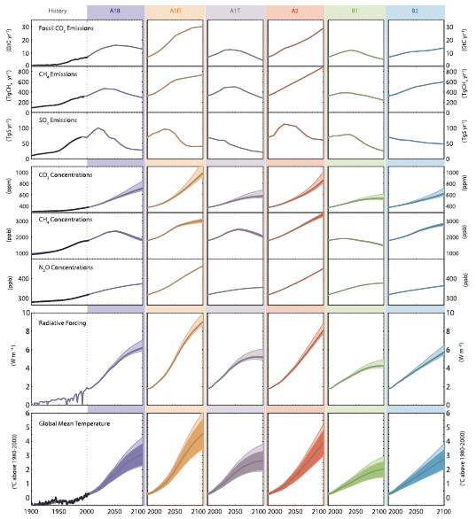
Figure 10.26. Fossil CO2,CH4 and SO2 emissions for six illustrative SRES non-mitigation emission scenarios, their corresponding CO2,CH4 andN2Oconcentrations, radiative forcing and global mean temperature projections based on an SCM tuned to 19 AOGCMs. The dark shaded areas in the bottom temperature panel represent the mean ±1 standard deviation for the 19 model tunings. The lighter shaded areas depict the change in this uncertainty range, if carbon cycle feedbacks are assumed to be lower or higher than in the medium setting. Mean projections for mid-range carbon cycle assumptions for the six illustrative SRES scenarios are shown as thick coloured lines. Historical emissions (black lines) are shown for fossil and industrial CO2 ( Marland et al., 2005 [NPR] ), for SO2 ( van Aardenne et al., 2001 [JoC] ) and for CH4 ( van Aardenne et al., 2001 [JoC] , adjusted to Olivier and Berdowski, 2001 [NPR] ). Observed CO2,CH4 andN2Oconcentrations (black lines) are as presented in Chapter6 .Global mean temperature results from the SCM for anthropogenic and natural forcing compare favourably with 20th-century observations (black line) as shown in the lower left panel ( Folland et al., 2001 [PoC, JoC, ARC] ; Jones et al., 2001 [JoC, ARC] ; Jones and Moberg, 2003 [JoC, ARC] ).
The radiative forcing projections in Figure 10.26 combine anthropogenic and natural (solar and volcanic) forcing. The forcing plumes reflect primarily the sensitivity of the forcing to carbon cycle uncertainties. Results are based on a forcing of 3.71 Wm–2 for a doubling of the atmospheric CO2 concentration. The anthropogenic forcing is based on Table 2.12 but uses a value of –0.8 Wm–2 for the present-day indirect aerosol forcing. Solar forcing for the historical period is prescribed according to Lean et al. 1995 [PoC, JoC, ARC] ) and volcanic forcing according to Ammann et al. 2003 [PoC, JoC, MoS, SRC] ). The historical solar forcing series is extended into the future using its average over the most recent 22 years. The volcanic forcing is adjusted to have a zero mean over the past 100 years and the anomaly is assumed to be zero for the future. In the TAR, the anthropogenic forcing was used alone even though the projections started in 1765 . There are several advantages of using both natural and anthropogenic forcing for the past. First, this was done by most of the AOGCMs the simple models are emulating. Second, it allows the simulations to be compared with observations. Third, the warming commitments accrued over the instrumental period are reflected in the projections. The disadvantage of including natural forcing is that the warming projections in 2100 are dependent to a few tenths of a degree on the necessary assumptions made about the natural forcing ( Bertrand et al., 2002 [JoC, MoS, ARC] ). These assumptions include how the natural forcing is projected into the future and whether to reference the volcanic forcing to a past reference period mean value. In addition, the choice of data set for both solar and volcanic forcing affects the results (see Section 2.7 for discussion about uncertainty in natural forcings).
The temperature projections for the six illustrative scenarios are shown in the bottom panel of Figure 10.26 .Model results are shown as anomalies from the mean of observations ( Folland et al., 2001 [PoC, JoC, ARC] ; Jones et al., 2001 [JoC, ARC] ; Jones and Moberg, 2003 [JoC, ARC] ) over the 1980 to 2000 period and the corresponding observed temperature anomalies are shown for comparison. The inner (darker) plumes show the ±1 standard deviation uncertainty due to the 19 model tunings and the outer (lighter) plumes show results for the corresponding high and low carbon cycle settings. Note that the asymmetry in the carbon cycle uncertainty causes global mean temperature projections to be skewed towards higher warming.
Considering only the mean of the SCM results with mid-range carbon cycle settings, the projected global mean temperature rise above 1980 to 2000 levels for the lower-emission SRES scenario B1 is 2.0°C in 2100 . For a higher-emission scenario, for example, the SRES A2 scenario, the global mean temperature is projected to rise by 3.9°C above 1980 to 2000 levels in 2100 . This clear difference in projected mean warming highlights the importance of assessing different emission scenarios separately. As mentioned above, the ‘response uncertainty’ is defined as the range in projections for a particular emission scenario. For the A2 emission scenario, the temperature change projections with the SCM span a ±1 standard deviation range of about 1.8°C, from 3.0°C to 4.8°C above 1980 to 2000 levels in 2100 . If carbon cycle feedbacks are considered to be low, the lower end of this range decreases only slightly and is unchanged to one decimal place. For the higher carbon cycle feedback settings, the upper bound of the ±1 standard deviation range increases to 5.2°C. For lower-emission scenarios, this uncertainty range is smaller. For example, the B1 scenario projections span a range of about 1.4°C, from 1.5°C to 2.9°C, including carbon cycle uncertainties. The corresponding results for the medium-emission scenario A1B are 2.3°C to 4.3°C, and for the higher-emission scenario A1FI, they are 3.4°C to 6.1°C. Note that these uncertainty ranges are not the minimum to maximum bounds of the projected warming across all SCM runs, which are higher, namely 2.7°C to 7.1°C for the A2 scenario and 1.3°C to 4.2°C for the B1 scenario (not shown).
The SCM results presented here are a sensitivity study with different model tunings and carbon cycle feedback parameters. Note that forcing uncertainties have not been assessed and that the AOGCM model results available for SCM tuning may not span the full range of possible climate response. For example, studies that constrain forecasts based on model fits to historic or present-day observations generally allow for a somewhat wider ‘response uncertainty’ (see Section 10.5.4 ). The concatenation of all such uncertainties would require a probabilistic approach because the extreme ranges have low probability. A synthesis of the uncertainty in global temperature increase by the year 2100 is provided in Section 10.5.4.6 .
10.5.4 Sampling Uncertainty and Estimating Probabilities
Uncertainty in the response of an AOGCM arises from the effects of internal variability, which can be sampled in isolation by creating ensembles of simulations of a single model using alternative initial conditions, and from modelling uncertainties, which arise from errors introduced by the discretization of the equations of motion on a finite resolution grid, and the parametrization of sub-grid scale processes (radiative transfer, cloud formation, convection, etc). Modelling uncertainties are manifested in alternative structural choices (for example, choices of resolution and the basic physical assumptions on which parametrizations are based), and in the values of poorly constrained parameters within parametrization schemes. Ensemble approaches are used to quantify the effects of uncertainties arising from variations in model structure and parameter settings. These are assessed in Sections 10.5.4.1 to 10.5.4.3 ,followed by a discussion of observational constraints in Section 10.5.4.4 and methods used to obtain probabilistic predictions in Sections 10.5.4.5 to 10.5.4.7 .
While ensemble projections carried out to date give a wide range of responses, they do not sample all possible sources of modelling uncertainty. For example, the AR4 multi-model ensemble relies on specified concentrations of CO2,thus neglecting uncertainties in carbon cycle feedbacks (see Section 10.4.1 ), although this can be partially addressed by using less detailed models to extrapolate the AOGCM results (see Section 10.5.3 ). More generally, the set of available models may share fundamental inadequacies, the effects of which cannot be quantified ( Kennedy and O’Hagan, 2001 [MoS] ). For example, climate models currently implement a restricted approach to the parametrization of sub-grid scale processes, using deterministic bulk formulae coupled to the resolved flow exclusively at the grid scale. Palmer et al. 2005 [Ambiguous] ) argue that the outputs of parametrization schemes should be sampled from statistical distributions consistent with a range of possible sub-grid scale states, following a stochastic approach that has been tried in numerical weather forecasting (e.g., Buizza et al., 1999 [JoC, MoS, SRC] ; Palmer, 2001 [JoC, MoS, SRC] ). The potential for missing or inadequately parametrized processes to broaden the simulated range of future changes is not clear, however, this is an important caveat for the results discussed below.
10.5.4.1 The Multi-Model Ensemble Approach
The use of ensembles of AOGCMs developed at different modelling centres has become established in climate prediction/ projection on both seasonal-to-interannual and centennial time scales. To the extent that simulation errors in different AOGCMs are independent, the mean of the ensemble can be expected to outperform individual ensemble members, thus providing an improved ‘best estimate’ forecast. Results show this to be the case, both in verification of seasonal forecasts ( Palmer et al., 2004 [JoC, MoS, SRC] ; Hagedorn et al., 2005 [JoC, MoS, SRC] ) and of the present-day climate from long term simulations ( Lambert and Boer, 2001 [JoC, MoS] ). By sampling modelling uncertainties, ensembles of AOGCMs should provide an improved basis for probabilistic projections compared with ensembles of a single model sampling only uncertainty in the initial state ( Palmer et al., 2005 [Ambiguous] ). However, members of a multi-model ensemble share common systematic errors ( Lambert and Boer, 2001 [JoC, MoS] ), and cannot span the full range of possible model configurations due to resource constraints. Verification of future climate change projections is not possible, however, Räisänen and Palmer 2001 [JoC, MoS, SRC] ) used a ‘perfect model approach’ (treating one member of an ensemble as truth and predicting its response using the other members) to show that the hypothetical economic costs associated with climate events can be reduced by calculating the probability of the event across the ensemble, rather than using a deterministic prediction from an individual ensemble member.
An additional strength of multi-model ensembles is that each member is subjected to careful testing in order to obtain a plausible and stable control simulation, although the process of tuning model parameters to achieve this( Section 8.1.3.1 )involves subjective judgement, and is not guaranteed to identify the optimum location in the model parameter space.
10.5.4.2 Perturbed Physics Ensembles
The AOGCMs featured in Section 10.5.2 are built by selecting components from a pool of alternative parametrizations, each based on a given set of physical assumptions and including a number of uncertain parameters. In principle, the range of predictions consistent with these components could be quantified by constructing very large ensembles with systematic sampling of multiple options for parametrization schemes and parameter values, while avoiding combinations likely to double-count the effect of perturbing a given physical process. Such an approach has been taken using simple climate models and EMICs ( Wigley and Raper, 2001 [PoC, JoC, MoS, SRC] ; Knutti et al., 2002 [Ambiguous] and Murphy et al. 2004 [JoC, MoS, SRC] and Stainforth et al. 2005 [JoC, MoS, SRC] ) describe the first steps in this direction using AOGCMs, constructing large ensembles by perturbing poorly constrained parameters in the atmospheric component of UKMO-HadCM3 coupled to a mixed layer ocean. These experiments quantify the range of equilibrium responses to doubled atmospheric CO2 consistent with uncertain parameters in a single GCM. Murphy et al. 2004 [JoC, MoS, SRC] ) perturbed 29 parameters one at a time, assuming that effects of individual parameters were additive but making a simple allowance for additional uncertainty introduced by nonlinear interactions. They find a probability distribution for climate sensitivity with a 5 to 95% range of 2.4°C to 5.4°C when weighting the models with a broadly based metric of the agreement between simulated and observed climatology, compared to 1.9°C to 5.3°C when all model versions are assumed equally reliable( Box 10.2 ,Figure 1c).
Stainforth et al. 2005 [JoC, MoS, SRC] ) deployed a distributed computing approach ( Allen, 1999 [JoC, MoS, SRC] ) to run a very large ensemble of 2,578 simulations sampling combinations of high, intermediate and low values of six parameters known to affect climate sensitivity. They find climate sensitivities ranging from 2°C to 11°C, with 4.2% of model versions exceeding 8°C, and show that the high-sensitivity models cannot be ruled out, based on a comparison with surface annual mean climatology. By utilising multivariate linear relationships between climate sensitivity and spatial fields of several present-day observables, the 5 to 95% range of climate sensitivity is estimated at 2.2°C to 6.8°C from the same data set ( Piani et al., 2005 [JoC, MoS, SRC] ; Box 10.2 Figure 1c). In this ensemble, Knutti et al. 2006 [JoC, SRC] ) find a strong relationship between climate sensitivity and the amplitude of the seasonal cycle in surface temperature in the present-day simulations. Most of the simulations with high sensitivities overestimate the observed amplitude. Based on this relationship, the 5 to 95% range of climate sensitivity is estimated at 1.5°C to 6.4°C( Box 10.2 ,Figure 1c). The differences between the PDFs in Box 10.2 ,Figure 1c, which are all based on the same climate model, reflect uncertainties in methodology arising from choices of uncertain parameters, their expert-specified prior distributions and alternative applications of observational constraints. They do not account for uncertainties associated with changes in ocean circulation, and do not account for structural model errors ( Smith, 2002 [JoC, MoS] ; Goldstein and Rougier, 2004 [MoS] )
Annan et al. 2005a [JoC, MoS, SRC] ) use an ensemble Kalman Filter technique to obtain uncertainty ranges for model parameters in an EMIC subject to the constraint of minimising simulation errors with respect to a set of climatological observations. Using this method, Hargreaves and Annan 2006 [JoC, MoS, SRC] ) find that the risk of a collapse in the Atlantic MOC (in response to increasing CO2)depends on the set of observations to which the EMIC parameters are tuned. Section 9.6.3 assesses perturbed physics studies of the link between climate sensitivity and cooling during the Last Glacial Maximum ( Annan et al., 2005b [MoS, SRC] ; Schneider von Deimling et al., 2006 [PoC, JoC, MoS, ARC] ).
10.5.4.3 Diagnosing Drivers of Uncertainty from Ensemble Results
Figure 10.27 ashows the agreement between annual changes simulated by members of the AR4 multi-model ensemble for 2080 to 2099 relative to 1980 to 1999 for the A1B scenario, calculated as in Räisänen 2001 [JoC, SRC] ). For precipitation, the agreement increases with spatial scale. For surface temperature, the agreement is high even at local scales, indicating the robustness of the simulated warming (see also Figure 10.8 ,discussed in Section 10.3.2.1 ). Differences in model formulation are the dominant contributor to ensemble spread, though the role of internal variability increases at smaller scales( Figure 10.27 b). The agreement between AR4 ensemble members is slightly higher compared with the earlier CMIP2 ensemble of Räisänen 2001 [JoC, SRC] ) (also reported in the TAR), and internal variability explains a smaller fraction of the ensemble spread. This is expected, given the larger forcing and responses in the A1B scenario for 2080 to 2099 compared to the transient response to doubled CO2 considered by Räisänen 2001 [JoC, SRC] ), although the use of an updated set of models may also contribute. For seasonal changes, internal variability is found to be comparable with model differences as a source of uncertainty in local precipitation and SLP changes (although not for surface temperature) in both multi-model and perturbed physics ensembles ( Räisänen, 2001 [JoC, SRC] ; Murphy et al., 2004 [JoC, MoS, SRC] ). Consequently the local seasonal changes for precipitation and SLP are not consistent in the AR4 ensemble over large areas of the globe (i.e., the multi-model mean change does not exceed the ensemble standard deviation; see Figure 10.9 ), whereas the surface temperature changes are consistent almost everywhere, as discussed in Section 10.3.2.1 .
Figure 10.27. Statistics of annual mean responses to the SRES A1B scenario, for 2080 to 2099 relative to 1980 to 1999, calculated from the 21-member AR4 multi-model ensemble using the methodology of Räisänen 2001 [JoC, SRC] ). Results are expressed as a function of horizontal scale on the x axis (‘Loc’: grid box scale; ‘Hem’: hemispheric scale; ‘Glob’: global mean) plotted against the y axis showing (a) the relative agreement between ensemble members, a dimensionless quantity defined as the square of the ensemble-mean response (corrected to avoid sampling bias) divided by the mean squared response of individual ensemble members, and (b) the dimensionless fraction of internal variability relative to the ensemble variance of responses. Values are shown for surface air temperature, precipitation and sea level pressure. The low agreement of SLP changes at hemispheric and global scales reflects problems with the conservation of total atmospheric mass in some of the models, however, this has no practical significance because SLP changes at these scales are extremely small.
Wang and Swail 2006b [JoC, MoS] ) examine the relative importance of internal variability, differences in radiative forcing and model differences in explaining the transient response of ocean wave height using three AOGCMs each run for three plausible forcing scenarios, and find model differences to be the largest source of uncertainty in the simulated changes.
Selten et al. 2004 [JoC, MoS] ) report a 62-member initial condition ensemble of simulations of 1940 to 2080 including natural and anthropogenic forcings. They find an individual member that reproduces the observed trend in the NAO over the past few decades, but no trend in the ensemble mean, and suggest that the observed change can be explained through internal variability associated with a mode driven by increases in precipitation over the tropical Indian Ocean. Terray et al. 2004 [JoC, MoS, SRC] ) find that the ARPEGE coupled ocean-atmosphere model shows small increases in the residence frequency of the positive phase of the NAO in response to SRES A2 and B2 forcing, whereas larger increases are found when SST changes prescribed from the coupled experiments are used to drive a version of the atmosphere model with enhanced resolution over the North Atlantic and Europe ( Gibelin and Déqué, 2003 [JoC, MoS] ).
Figure 10.25 compares global mean transient and equilibrium changes simulated by the AR4 multi-model ensembles against perturbed physics ensembles (M. Collins et al., 2006 [Ambiguous] ; Webb et al., 2006 [JoC, ARC] ) designed to produce credible present-day simulations while sampling a wide range of multiple parameter perturbations and climate sensitivities. The AR4 ensembles partially sample structural variations in model components, whereas the perturbed physics ensembles sample atmospheric parameter uncertainties for a fixed choice of model structure. The results show similar relationships between TCR, climate sensitivity and precipitation change in both types of ensemble. The perturbed physics ensembles contain several members with sensitivities higher than the multi-model range, while some of the multi-model transient simulations give TCR values slightly below the range found in the perturbed physics ensemble( Figure 10.25 a,b).
Soden and Held 2006 [JoC, MoS, ARC] ) find that differences in cloud feedback are the dominant source of uncertainty in the transient response of surface temperature in the AR4 ensemble (see also Section 8.6.3.2 ), as in previous IPCC assessments. Webb et al. 2006 [JoC, ARC] ) compare equilibrium radiative feedbacks in a 9-member multi-model ensemble against those simulated in a 128-member perturbed physics ensemble with multiple parameter perturbations. They find that the ranges of climate sensitivity in both ensembles are explained mainly by differences in the response of shortwave cloud forcing in areas where changes in low-level clouds predominate. Bony and Dufresne 2005 [JoC, MoS, ARC] ) find that marine boundary layer clouds in areas of large-scale subsidence provide the largest source of spread in tropical cloud feedbacks in the AR4 ensemble. Narrowing the uncertainty in cloud feedback may require both improved parametrizations of cloud microphysical properties (e.g., Tsushima et al., 2006 [JoC, MoS] ) and improved representations of cloud macrophysical properties, through improved parametrizations of other physical processes (e.g., Williams et al., 2001 [JoC, MoS, ARC] ) and/or increases in resolution ( Palmer, 2005 [Ambiguous] ).
10.5.4.4 Observational Constraints
Arange of observables has been used since the TAR to explore methods for constraining uncertainties in future climate change in studies using simple climate models, EMICs and AOGCMs. Probabilistic estimates of global climate sensitivity have been obtained from the historical transient evolution of surface temperature, upper-air temperature, ocean temperature, estimates of the radiative forcing, satellite data, proxy data over the last millennium, or a subset thereof ( Wigley et al., 1997a [PoC, JoC, SRC] ; Tol and de Vos, 1998 [JoC] ; Andronova and Schlesinger, 2001 [JoC, MoS, ARC] ; Forest et al., 2002 [JoC, ARC] ; Gregory et al., 2002a [JoC, MoS, SRC] ; Knutti et al., 2002 [Ambiguous] , 2003; Frame et al., 2005 [JoC, MoS] ; Forest et al., 2006 [JoC, MoS, SRC] ; Forster and Gregory, 2006 [JoC, SRC] ; Hegerl et al., 2006 [PoC, JoC, SRC] ; see Section 9.6 ). Some of these studies also constrain the transient response to projected future emissions (see section 10.5.4.5 ). For climate sensitivity, further probabilistic estimates have been obtained using statistical measures of the correspondence between simulated and observed fields of present-day climate ( Murphy et al., 2004 [JoC, MoS, SRC] ; Piani et al., 2005 [JoC, MoS, SRC] ), the climatological seasonal cycle of surface temperature ( Knutti et al., 2006 [JoC, SRC] ) and the response to palaeoclimatic forcings ( Annan et al., 2005b [MoS, SRC] ; Schneider von Deimling et al., 2006 [PoC, JoC, MoS, ARC] ). For the purpose of constraining regional climate projections, spatial averages or fields of time-averaged regional climate have been used ( Giorgi and Mearns, 2003 [JoC, ARC] ; Tebaldi et al., 2004 [JoC, MoS, SRC] , 2005; Laurent and Cai, 2007 [JoC, 2007] ), as have past regional- or continental-scale trends in surface temperature ( Greene et al., 2006 [JoC, MoS] ; Stott et al., 2006a [JoC, MoS, SRC] ).
Further observables have been suggested as potential constraints on future changes, but are not yet used in formal probabilistic estimates. These include measures of climate variability related to cloud feedbacks ( Bony et al., 2004 [JoC, ARC] ; Bony and Dufresne, 2005 [JoC, MoS, ARC] ; Williams et al., 2005 [JoC, MoS] ), radiative damping of the seasonal cycle ( Tsushima et al., 2005 [JoC, MoS] ), the relative entropy of simulated and observed surface temperature variations ( Shukla et al., 2006 [JoC, MoS, ARC] ), major volcanic eruptions ( Wigley et al., 2005 [PoC, JoC, SRC] ; Yokohata et al., 2005 [JoC, MoS] ; see Section 9.6 )and trends in multiple variables derived from reanalysis data sets ( Lucarini and Russell, 2002 [JoC, MoS, SRC] ).
Additional constraints could also be found, for example, from evaluation of ensemble climate prediction systems on shorter time scales for which verification data exist. These could include assessment of the reliability of seasonal to interannual probabilistic forecasts ( Palmer et al., 2004 [JoC, MoS, SRC] ; Hagedorn et al., 2005 [JoC, MoS, SRC] ) and the evaluation of model parametrizations in short-range weather predictions ( Phillips et al., 2004 [JoC, MoS, ARC] ; Palmer, 2005 [Ambiguous] Annan and Hargreaves 2006 [JoC, MoS, SRC] ) point out the potential for narrowing uncertainty by combining multiple lines of evidence. This will require objective quantification of the impact of different constraints and their degree of independence, estimation of the effects of structural modelling errors and the development of comprehensive probabilistic frameworks in which to combine these elements (e.g., Rougier, 2007 [JoC, MoS, 2007] ).
10.5.4.5 Probabilistic Projections - Global Mean
Anumber of methods for providing probabilistic climate change projections, both for global means (discussed in this section) and geographical depictions (discussed in the following section) have emerged since the TAR.
Methods of constraining climate sensitivity using observations of present-day climate are discussed in Section 10.5.4.2 .Results from both the AR4 multi-model ensemble and from perturbed physics ensembles suggest a very low probability for a climate sensitivity below 2°C, despite exploring the effects of a wide range of alternative modelling assumptions on the global radiative feedbacks arising from lapse rate, water vapour, surface albedo and cloud ( Bony et al., 2006 [JoC, ARC] ; Soden and Held, 2006 [JoC, MoS, ARC] ; Webb et al., 2006 [JoC, ARC] ; Box 10.2 ). However, exclusive reliance on AOGCM ensembles can be questioned on the basis that models share components, and therefore errors, and may not sample the full range of possible outcomes (e.g., Allen and Ingram, 2002 [JoC, MoS, SRC] ).
Observationally constrained probability distributions for climate sensitivity have also been derived from physical relationships based on energy balance considerations, and from instrumental observations of historical changes during the past 50 to 150 years or proxy reconstructions of surface temperature during the past millennium( Section 9.6 ). The results vary according to the choice of verifying observations, the forcings considered and their specified uncertainties, however, all these studies report a high upper limit for climate sensitivity, with the 95th percentile of the distributions invariably exceeding 6°C( Box 10.2 Frame et al. 2005 [JoC, MoS] ) demonstrate that uncertainty ranges for sensitivity are dependent on the choices made about prior distributions of uncertain quantities before the observations are applied. Frame et al. 2005 [JoC, MoS] and Piani et al. 2005 [JoC, MoS, SRC] ) show that many observable variables are likely to scale inversely with climate sensitivity, implying that projections of quantities that are inversely related to sensitivity will be more strongly constrained by observations than climate sensitivity itself, particularly with respect to the estimated upper limit ( Allen et al., 2006b [NPR, SRC] ).
In the case of transient climate change, optimal detection techniques have been used to determine factors by which hindcasts of global surface temperature from AOGCMs can be scaled up or down while remaining consistent with past changes, accounting for uncertainty due to internal variability( Section 9.4.1.6 ). Uncertainty is propagated forward in time by assuming that the fractional error found in model hindcasts of global mean temperature change will remain constant in projections of future changes. Using this approach, Stott and Kettleborough 2002 [JoC, MoS, SRC] ) find that probabilistic projections of global mean temperature derived from UKMO-HadCM3 simulations were insensitive to differences between four representative SRES emissions scenarios over the first few decades of the 21st century, but that much larger differences emerged between the response to different SRES scenarios by the end of the 21st century (see also Section 10.5.3 and Figure 10.28 Stott et al. 2006b [JoC, MoS, SRC] ) show that scaling the responses of three models with different sensitivities brings their projections into better agreement. Stott et al. 2006a [JoC, MoS, SRC] ) extend their approach to obtain probabilistic projections of future warming averaged over continental-scale regions under the SRES A2 scenario. Fractional errors in the past continental warming simulated by UKMO-HadCM3 are used to scale future changes, yielding wide uncertainty ranges, notably for North America and Europe where the 5 to 95% ranges for warming during the 21st century are 2°C to 12°C and 2°C to 11°C respectively. These estimates do not account for potential constraints arising from regionally differentiated warming rates. Tighter ranges of 4°C to 8°C for North America and 4°C to 7°C for Europe are obtained if fractional errors in past global mean temperature are used to scale the future continental changes, although this neglects uncertainty in the relationship between global and regional temperature changes.
Allen and Ingram 2002 [JoC, MoS, SRC] ) suggest that probabilistic projections for some variables may be made by searching for ‘emergent constraints’. These are relationships between variables that can be directly constrained by observations, such as global surface temperature, and variables that may be indirectly constrained by establishing a consistent, physically based relationship which holds across a wide range of models. They present an example in which future changes in global mean precipitation are constrained using a probability distribution for global temperature obtained from a large EMIC ensemble ( Forest et al., 2002 [JoC, ARC] ) and a relationship between precipitation and temperature obtained from multi-model ensembles of the response to doubled atmospheric CO2.These methods are designed to produce distributions constrained by observations, and are relatively model independent ( Allen and Stainforth, 2002 [JoC, MoS, SRC] ; Allen et al., 2006a [NPR, MoS, SRC] ). This can be achieved provided the inter-variable relationships are robust to alternative modelling assumptions Piani et al. 2005 [JoC, MoS, SRC] and Knutti et al. 2006 [JoC, SRC] ) (described in Section 10.5.4.2 )follow this approach, noting that in these cases the inter-variable relationships are derived from perturbed versions of a single model, and need to be confirmed using other models.
Asynthesis of published probabilistic global mean projections for the SRES scenarios B1, A1B and A2 is given in Figure 10.28 .Probability density functions are given for short-term projections ( 2020 – 2030 ) and the end of the century ( 2090 – 2100 ). For comparison, normal distributions fitted to results from AOGCMs in the multi-model archive (see Section 10.3.1 )are also given, although these curve fits should not be regarded as PDFs. The five methods of producing PDFs are all based on different models and/or techniques, described in Section 10.5 .In short, Wigley and Raper 2001 [PoC, JoC, MoS, SRC] ) use a large ensemble of a simple model with expert prior distributions for climate sensitivity, ocean heat uptake, sulphate forcing and the carbon cycle, without applying constraints. Knutti et al. 2002 [Ambiguous] , 2003 ) use a large ensemble of EMIC simulations with non-informative prior distributions, consider uncertainties in climate sensitivity, ocean heat uptake, radiative forcing and the carbon cycle, and apply observational constraints. Neither method considers natural variability explicitly. Stott et al. 2006b [JoC, MoS, SRC] ) apply the fingerprint scaling method to AOGCM simulations to obtain PDFs which implicitly account for uncertainties in forcing, climate sensitivity and internal unforced as well as forced natural variability. For the A2 scenario, results obtained from three different AOGCMs are shown, illustrating the extent to which the Stott et al. PDFs depend on the model used. Harris et al. 2006 [JoC, MoS, SRC] ) obtain PDFs by boosting a 17-member perturbed physics ensemble of the UKMO-HadCM3 model using scaled equilibrium responses from a larger ensemble of simulations. Furrer et al. 2007 [NPR, MoS, SRC, 2007] ) use a Bayesian method described in Section 10.5.4.7 to calculate PDFs from the AR4 multi-model ensemble. The Stott et al. 2006b [JoC, MoS, SRC] Harris et al. 2006 [JoC, MoS, SRC] and Furrer et al. 2007 [NPR, MoS, SRC, 2007] ) methods neglect carbon cycle uncertainties.
Figure 10.28. Probability density functions from different studies for global mean temperature change for the SRES scenarios B1, A1B and A2 and for the decades 2020 to 2029 and 2090 to 2099 relative to the 1980 to 1999 average ( Wigley and Raper, 2001 [PoC, JoC, MoS, SRC] ; Knutti et al., 2002 [Ambiguous] ; Furrer et al., 2007 [NPR, MoS, SRC, 2007] ; Harris et al., 2006 [JoC, MoS, SRC] ; Stott et al., 2006b [JoC, MoS, SRC] ). A normal distribution fitted to the multi-model ensemble is shown for comparison.
Two key points emerge from Figure 10.28 .For the projected short-term warming (i) there is more agreement among models and methods (narrow width of the PDFs) compared to later in the century (wider PDFs), and (ii) the warming is similar across different scenarios, compared to later in the century where the choice of scenario significantly affects the projections. These conclusions are consistent with the results obtained with SCMs( Section 10.5.3 ).
Additionally, projection uncertainties increase close to linearly with temperature in most studies. The different methods show relatively good agreement in the shape and width of the PDFs, but with some offsets due to different methodological choices. Only Stott et al. 2006b [JoC, MoS, SRC] ) account for variations in future natural forcing, and hence project a small probability of cooling over the next few decades not seen in the other PDFs. The results of Knutti et al. 2003 [PoC, JoC, MoS, SRC] ) show wider PDFs for the end of the century because they sample uniformly in climate sensitivity (see Section 9.6.2 and Box 10.2 ). Resampling uniformly in observables ( Frame et al., 2005 [JoC, MoS] ) would bring their PDFs closer to the others. In sum, probabilistic estimates of uncertainties for the next few decades seem robust across a variety of models and methods, while results for the end of the century depend on the assumptions made.
10.5.4.6 Synthesis of Projected Global Temperature at Year 2100
All available estimates for projected warming by the end of the 21st century are summarised in Figure 10.29 for the six SRES non-intervention marker scenarios. Among the various techniques, the AR4 AOGCM ensemble provides the most sophisticated set of models in terms of the range of processes included and consequent realism of the simulations compared to observations (see Chapters 8 and 9 ). On average, this ensemble projects an increase in global mean surface air temperature of 1.8°C, 2.8°C and 3.4°C in the B1, A1B and A2 scenarios, respectively, by 2090 to 2099 relative to 1980 to 1999 (note that in Table 10.5 ,the years 2080 to 2099 were used for those globally averaged values to be consistent with the comparable averaging period for the geographic plots in Section 10.3 ;this longer averaging period smoothes spatial noise in the geographic plots). A scaling method is used to estimate AOGCM mean results for the three missing scenarios B2, A1T and A1FI. The ratio of the AOGCM mean values for B1 relative to A1B and A2 relative to A1B are almost identical to the ratios obtained with the MAGICC SCM, although the absolute values for the SCM are higher. Thus, the AOGCM mean response for the scenarios B2, A1T and A1FI can be estimated as 2.4°C, 2.4°C and 4.0°C by multiplying the AOGCM A1B mean by the SCM-derived ratios B2/A1B, A1T/A1B and A1FI/A1B, respectively (for details see Appendix 10 .A.1).
The AOGCMs cannot sample the full range of possible warming, in particular because they do not include uncertainties in the carbon cycle. In addition to the range derived directly from the AR4 multi-model ensemble, Figure 10.29 depicts additional uncertainty estimates obtained from published probabilistic methods using different types of models and observational constraints: the MAGICC SCM and the BERN2.5CC coupled climate-carbon cycle EMIC tuned to different climate sensitivities and carbon cycle settings, and theC4MIP coupled climate-carbon cycle models. Based on these results, the future increase in global mean temperature is likely to fall within –40 to +60% of the multi-model AOGCM mean warming simulated for each scenario. This range results from an expert judgement of the multiple lines of evidence presented in Figure 10.29 ,and assumes that the models approximately capture the range of uncertainties in the carbon cycle. The range is well constrained at the lower bound since climate sensitivity is better constrained at the low end (see Box 10.2 ), and carbon cycle uncertainty only weakly affects the lower bound. The upper bound is less certain as there is more variation across the different models and methods, partly because carbon cycle feedback uncertainties are greater with larger warming. The uncertainty ranges derived from the above percentages for the warming by 2090 to 2099 relative to 1980 to 1999 are 1.1°C to 2.9°C, 1.4°C to 3.8°C, 1.7°C to 4.4°C, 1.4°C to 3.8°C, 2.0°C to 5.4°C and 2.4°C to 6.4°C for the scenarios B1, B2, A1B, A1T, A2 and A1FI, respectively. It is not appropriate to compare the lowest and highest values across these ranges against the single range given in the TAR, because the TAR range resulted only from projections using an SCM and covered all SRES scenarios, whereas here a number of different and independent modelling approaches are combined to estimate ranges for the six illustrative scenarios separately. Additionally, in contrast to the TAR, carbon cycle uncertainties are now included in these ranges. These uncertainty ranges include only anthropogenically forced changes.
10.5.4.7 Probabilistic Projections - Geographical Depictions
Tebaldi et al. 2005 [JoC, MoS, SRC] ) present a Bayesian approach to regional climate prediction, developed from the ideas of Giorgi and Mearns 2002 [JoC, MoS, ARC] , 2003 ). Non-informative prior distributions for regional temperature and precipitation are updated using observations and results from AOGCM ensembles to produce probability distributions of future changes. Key assumptions are that each model and the observations differ randomly and independently from the true climate, and that the weight given to a model prediction should depend on the bias in its present-day simulation and its degree of convergence with the weighted ensemble mean of the predicted future change. Lopez et al. 2006 [JoC] ) apply the Tebaldi et al. 2005 [JoC, MoS, SRC] ) method to a 15-member multi-model ensemble to predict future changes in global surface temperature under a 1% yr–1 increase in atmospheric CO2.They compare it with the method developed by Allen et al. 2000 [JoC, MoS, SRC] and Stott and Kettleborough 2002 [JoC, MoS, SRC] ) (ASK), which aims to provide relatively model independent probabilities consistent with observed changes (see Section 10.5.4.5 ). The Bayesian method predicts a much narrower uncertainty range than ASK. However its results depend on choices made in its design, particularly the convergence criterion for up-weighting models close to the ensemble mean, relaxation of which substantially reduces the discrepancy with ASK.
Another method by Furrer et al. 2007 [NPR, MoS, SRC, 2007] ) employs a hierarchical Bayesian model to construct PDFs of temperature change at each grid point from a multi-model ensemble. The main assumptions are that the true climate change signal is a common large-scale structure represented to some degree in each of the model simulations, and that the signal unexplained by climate change is AOGCM-specific in terms of small-scale structure, but can be regarded as noise when averaged over all AOGCMs. In this method, spatial fields of future minus present temperature difference from each ensemble member are regressed upon basis functions. One of the basis functions is a map of differences of observed temperatures from late- minus mid-20th century, and others are spherical harmonics. The statistical model then estimates the regression coefficients and their associated errors, which account for the deviation in each AOGCM from the (assumed) true pattern of change. By recombining the coefficients with the basis functions, an estimate is derived of the true climate change field and its associated uncertainty, thus providing joint probabilities for climate change at all grid points around the globe.
Estimates of uncertainty derived from multi-model ensembles of 10 to 20 members are potentially sensitive to outliers ( Räisänen, 2001 [JoC, SRC] Harris et al. 2006 [JoC, MoS, SRC] ) therefore augment a 17-member ensemble of AOGCM transient simulations by scaling the equilibrium response patterns of a large perturbed physics ensemble. Transient responses are emulated by scaling equilibrium response patterns according to global temperature (predicted from an energy balance model tuned to the relevant climate sensitivities). For surface temperature, the scaled equilibrium patterns correspond well to the transient response patterns, while scaling errors for precipitation vary more widely with location. A correction field is added to account for ensemble-mean differences between the equilibrium and transient patterns, and uncertainty is allowed for in the emulated result. The correction field and emulation errors are determined by comparing the responses of model versions for which both transient and equilibrium simulations exist. Results are used to obtain frequency distributions of transient regional changes in surface temperature and precipitation in response to increasing atmospheric CO2,arising from the combined effects of atmospheric parameter perturbations and internal variability in UKMO-HadCM3.
Figure 10.30 shows probabilities of a temperature change larger than 2°C by the end of the 21st century under the A1B scenario, comparing values estimated from the 21-member AR4 multi-model ensemble ( Furrer et al., 2007 [NPR, MoS, SRC, 2007] ) against values estimated by combining transient and equilibrium perturbed physics ensembles of 17 and 128 members, respectively ( Harris et al., 2006 [JoC, MoS, SRC] ). Although the methods use different ensembles and different statistical approaches, the large-scale patterns are similar in many respects. Both methods show larger probabilities (typically 80% or more) over land, and at high latitudes in the winter hemisphere, with relatively low values (typically less than 50%) over the southern oceans. However, the plots also reveal some substantial differences at a regional level, notably over the North Atlantic Ocean, the sub-tropical Atlantic and Pacific Oceans in the SH, and at high northern latitudes during June to August.
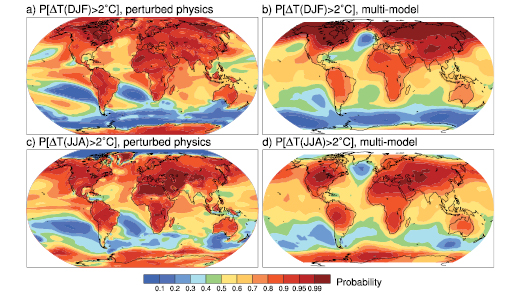
Figure 10.30. Estimated probabilities for a mean surface temperature change exceeding 2°C in 2080 to 2099 relative to 1980 to 1999 under the SRES A1B scenario. Results obtained from a perturbed physics ensemble of a single model (a, c), based on Harris et al. 2006 [JoC, MoS, SRC] ), are compared with results from the AR4 multi-model ensemble (b, d), based on Furrer et al. 2007 [NPR, MoS, SRC, 2007] ), for December to February (DJF, a, b) and June to August (JJA, c, d).
10.5.4.8 Summary
Significant progress has been made since the TAR in exploring ensemble approaches to provide uncertainty ranges and probabilities for global and regional climate change. Different methods show consistency in some aspects of their results, but differ significantly in others (see Box 10.2 ;Figures 10.28 and 10.30 ), because they depend to varying degrees on the nature and use of observational constraints, the nature and design of model ensembles and the specification of prior distributions for uncertain inputs (see, e.g., Table 11.3 ). A preferred method cannot yet be recommended, but the assumptions and limitations underlying the various approaches, and the sensitivity of the results to them, should be communicated to users. A good example concerns the treatment of model error in Bayesian methods, the uncertainty in which affects the calculation of the likelihood of different model versions, but is difficult to specify ( Rougier, 2007 [JoC, MoS, 2007] ). Awareness of this issue is growing in the field of climate prediction ( Annan et al., 2005b [MoS, SRC] ; Knutti et al., 2006 [JoC, SRC] ), however, it is yet to be thoroughly addressed. Probabilistic depictions, particularly at the regional level, are new to climate change science and are being facilitated by the recently available multi-model ensembles. These are discussed further in Section 11.10.2 .
10.6 Sea Level Change in the 21st Century
10.6.1 Global Average Sea Level Rise Due to Thermal Expansion
As seawater warms up, it expands, increasing the volume of the global ocean and producing thermosteric sea level rise (see Section 5.5.3 ). Global average thermal expansion can be calculated directly from simulated changes in ocean temperature. Results are available from 17 AOGCMs for the 21st century for SRES scenarios A1B, A2 and B1( Figure 10.31 ), continuing from simulations of the 20th century. One ensemble member was used for each model and scenario. The time series are rather smooth compared with global average temperature time series, because thermal expansion reflects heat storage in the entire ocean, being approximately proportional to the time integral of temperature change ( Gregory et al., 2001 [JoC, SRC] ).
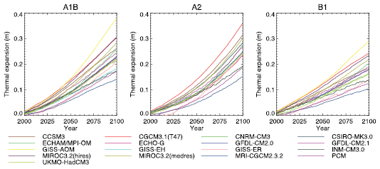
Figure 10.31. Projected global average sea level rise (m) due to thermal expansion during the 21st century relative to 1980 to 1999 under SRES scenarios A1B, A2 and B1. See Table 8.1 for model descriptions.
During 2000 to 2020 under scenario SRES A1B in the ensemble of AOGCMs, the rate of thermal expansion is 1.3 ± 0.7 mm yr–1,and is not significantly different under A2 or B1. This rate is more than twice the observationally derived rate of 0.42 ± 0.12 mm yr–1 during 1961 to 2003 . It is similar to the rate of 1.6 ± 0.5 mm yr–1 during 1993 to 2003 (see Section 5.5.3 ), which may be larger than that of previous decades partly because of natural forcing and internal variability (see Sections 5.5.2.4 , 5.5.3 and 9.5.2 ). In particular, many of the AOGCM experiments do not include the influence of Mt. Pinatubo, the omission of which may reduce the projected rate of thermal expansion during the early 21st century.
During 2080 to 2100, the rate of thermal expansion is projected to be 1.9 ± 1.0, 2.9 ± 1.4 and 3.8 ± 1.3 mm yr–1 under scenarios SRES B1, A1B and A2 respectively in the AOGCM ensemble (the width of the range is affected by the different numbers of models under each scenario). The acceleration is caused by the increased climatic warming. Results are shown for all SRES marker scenarios in Table 10.7 (see Appendix 10.A for methods). In the AOGCM ensemble, under any given SRES scenario, there is some correlation of the global average temperature change across models with thermal expansion and its rate of change, suggesting that the spread in thermal expansion for that scenario is caused both by the spread in surface warming and by model-dependent ocean heat uptake efficiency ( Raper et al., 2002 [JoC, SRC] ; Table 8.2 )and the distribution of added heat within the ocean ( Russell et al., 2000 [JoC, MoS, SRC] ).
10.6.2 Local Sea Level Change Due to Change in Ocean Density and Dynamics
The geographical pattern of mean sea level relative to the geoid (the dynamic topography) is an aspect of the dynamical balance relating the ocean’s density structure and its circulation, which are maintained by air-sea fluxes of heat, freshwater and momentum. Over much of the ocean on multi-annual time scales, a good approximation to the pattern of dynamic topography change is given by the steric sea level change, which can be calculated straightforwardly from local temperature and salinity change ( Gregory et al., 2001 [JoC, SRC] ; Lowe and Gregory, 2006 [JoC, MoS, SRC] ). In much of the world, salinity changes are as important as temperature changes in determining the pattern of dynamic topography change in the future, and their contributions can be opposed ( Landerer et al., 2007 [NPR, SRC, 2007] ; and as in the past, Section 5.5.4.1 Lowe and Gregory 2006 [JoC, MoS, SRC] ) show that in the UKMO-HadCM3 AOGCM, changes in heat fluxes are the cause of many of the large-scale features of sea level change, but freshwater flux change dominates the North Atlantic and momentum flux change has a signature in the north and low-latitude Pacific and the Southern Ocean.
Results are available for local sea level change due to ocean density and circulation change from AOGCMs in the multi-model ensemble for the 20th century and the 21st century. There is substantial spatial variability in all models (i.e., sea level change is not uniform), and as the geographical pattern of climate change intensifies, the spatial standard deviation of local sea level change increases ( Church et al., 2001 [NPR, ARC] ; Gregory et al., 2001 [JoC, SRC] Suzuki et al. 2005 [JoC, MoS] ) show that, in their high-resolution model, enhanced eddy activity contributes to this increase, but across models there is no significant correlation of the spatial standard deviation with model spatial resolution. This section evaluates sea level change between 1980 to 1999 and 2080 to 2099 projected by 16 models forced with SRES scenario A1B. (Other scenarios are qualitatively similar, but fewer models are available.) The ratio of spatial standard deviation to global average thermal expansion varies among models, but is mostly within the range 0.3 to 0.4. The model median spatial standard deviation of thermal expansion is 0.08 m, which is about 25% of the central estimate of global average sea level rise during the 21st century under A1B( Table 10.7 ).
The geographical patterns of sea level change from different models are not generally similar in detail, although they have more similarity than those analysed in the TAR by Church et al. 2001 [NPR, ARC] ). The largest spatial correlation coefficient between any pair is 0.75, but only 25% of correlation coefficients exceed 0.5. To identify common features, an ensemble mean( Figure 10.32 )is examined. There are only limited areas where the model ensemble mean change exceeds the inter-model standard deviation, unlike for surface air temperature change( Section 10.3.2.1 ).
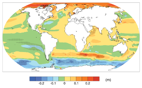
Figure 10.32. Local sea level change (m) due to ocean density and circulation change relative to the global average (i.e., positive values indicate greater local sea level change than global) during the 21st century, calculated as the difference between averages for 2080 to 2099 and 1980 to 1999, as an ensemble mean over 16 AOGCMs forced with the SRES A1B scenario. Stippling denotes regions where the magnitude of the multi-model ensemble mean divided by the multi-model standard deviation exceeds 1.0.
Like Church et al. 2001 [NPR, ARC] and Gregory et al. 2001 [JoC, SRC] ), Figure 10.32 shows smaller than average sea level rise in the Southern Ocean and larger than average in the Arctic, the former possibly due to wind stress change ( Landerer et al., 2007 [NPR, SRC, 2007] ) or low thermal expansivity ( Lowe and Gregory, 2006 [JoC, MoS, SRC] ) and the latter due to freshening. Another obvious feature is a narrow band of pronounced sea level rise stretching across the southern Atlantic and Indian Oceans and discernible in the southern Pacific. This could be associated with a southward shift in the circumpolar front ( Suzuki et al., 2005 [JoC, MoS] ) or subduction of warm anomalies in the region of formation of sub antarctic mode water ( Banks et al., 2002 [MoS, SRC] ). In the zonal mean, there are maxima of sea level rise in 30°S to 45°S and 30°N to 45°N. Similar indications are present in the altimetric and thermosteric patterns of sea level change for 1993 to 2003 ( Figure 5.15 ). The model projections do not share other aspects of the observed pattern of sea level rise, such as in the western Pacific, which could be related to interannual variability.
The North Atlantic dipole pattern noted by Church et al. 2001 [NPR, ARC] ), that is, reduced rise to the south of the Gulf Stream extension, enhanced to the north, consistent with a weakening of the circulation, is present in some models; a more complex feature is described by Landerer et al. 2007 [NPR, SRC, 2007] ). The reverse is apparent in the north Pacific, which Suzuki et al. 2005 [JoC, MoS] ) associate with a wind-driven intensification of the Kuroshio Current. Using simplified models, Hsieh and Bryan 1996 [JoC, MoS] ( and Johnson and Marshall 2002 ) ) show how upper-ocean velocities and sea level would be affected in North Atlantic coastal regions within months of a cessation of sinking in the North Atlantic as a result of propagation by coastal and equatorial Kelvin waves, but would take decades to adjust in the central regions and the south Atlantic. Levermann et al. 2005 [JoC, ARC] ) show that a sea level rise of several tenths of a metre could be realised in coastal regions of the North Atlantic within a few decades (i.e., tens of millimetres per year) of a collapse of the MOC. Such changes to dynamic topography would be much more rapid than global average sea level change. However, it should be emphasized that these studies are sensitivity tests, not projections; the Atlantic MOC does not collapse in the SRES scenario runs evaluated here (see Section 10.3.4 ).
The geographical pattern of sea level change is affected also by changes in atmospheric surface pressure, but this is a relatively small effect given the projected pressure changes( Figure 10.9 ;a pressure increase of 1 hPa causes a drop in local sea level of 0.01 m; see Section 5.5.4.3 ). Land movements and changes in the gravitational field resulting from the changing loading of the crust by water and ice also have effects which are small over most of the ocean (see Section 5.5.4.4 ).
10.6.3 Glaciers and Ice Caps
Glaciers and ice caps (G&IC, see also Section 4.5.1 )comprise all land ice except for the ice sheets of Greenland and Antarctica (see Sections 4.6.1 and 10.6.4 ). The mass of G&IC can change because of changes in surface mass balance( Section 10.6.3.1 ). Changes in mass balance cause changes in area and thickness( Section 10.6.3.2 ), with feedbacks on surface mass balance.
10.6.3.1 Mass Balance Sensitivity to Temperature and Precipitation
Since G&IC mass balance depends strongly on their altitude and aspect, use of data from climate models to make projections requires a method of downscaling, because individual G&IC are much smaller than typical AOGCM grid boxes. Statistical relations for meteorological quantities can be developed between the GCM and local scales ( Reichert et al., 2002 [JoC, SRC] ), but they may not continue to hold in future climates. Hence, for projections the approach usually adopted is to use GCM simulations of changes in climate parameters to perturb the observed climatology or mass balance ( Gregory and Oerlemans, 1998 [JoC, MoS, SRC] ; Schneeberger et al., 2003 [MoS, SRC] ).
Change in ablation (mostly melting) of a glacier or ice cap is modelled using bT (in m yr–1 °C–1), the sensitivity of the mean specific surface mass balance to temperature (refer to Section 4.5 for a discussion of the relation of mass balance to climate). One approach determines bT by energy balance modelling, including evolution of albedo and refreezing of melt water within the firn ( Zuo and Oerlemans, 1997 [JoC, SRC] Oerlemans and Reichert 2000 [SRC] Oerlemans 2001 [NPR, SRC] and Oerlemans et al. 2006 [MoS, SRC] ) refine this approach to include dependence on monthly temperature and precipitation changes. Another approach uses a degree-day method, in which ablation is proportional to the integral of mean daily temperature above the freezing point ( Braithwaite et al., 2003 [SRC] Braithwaite and Raper 2002 [SRC] ) show that there is excellent consistency between the two approaches, which indicates a similar relationship between bT and climatological precipitation. Schneeberger et al. 2000 [JoC] , 2003 ) use a degree-day method for ablation modified to include incident solar radiation, again obtaining similar results. de Woul and Hock 2006 [ARC] ) find somewhat larger sensitivities for arctic G&IC from the degree-day method than the energy balance method. Calculations of bT are estimated to have an uncertainty of ±15% (standard deviation) ( Gregory and Oerlemans, 1998 [JoC, MoS, SRC] ; Raper and Braithwaite, 2006 [JoC, MoS, SRC] ).
The global average sensitivity of G&IC surface mass balance to temperature is estimated by weighting the local sensitivities by land ice area in various regions. For a geographically and seasonally uniform rise in global temperature, Oerlemans and Fortuin 1992 [JoC, SRC] ) derive a global average G&IC surface mass balance sensitivity of –0.40 m yr–1 °C–1 ,Dyurgerov and Meier 2000 [JoC, SRC] ) –0.37 m yr–1 °C–1 (from observations), Braithwaite and Raper 2002 [SRC] ) –0.41 m yr–1 °C–1 and Raper and Braithwaite 2005 [JoC, MoS, SRC] ) –0.35 m yr–1 °C–1.Applying the scheme of Oerlemans 2001 [NPR, SRC] and Oerlemans et al. 2006 [MoS, SRC] ) worldwide gives a smaller value of –0.32 m yr–1 °C–1,the reduction being due to the modified treatment of albedo by Oerlemans 2001 [NPR, SRC] ).
These global average sensitivities for uniform temperature change are given only for scenario-independent comparison of the various methods; they cannot be used for projections, which require regional and seasonal temperature changes ( Gregory and Oerlemans, 1998 [JoC, MoS, SRC] ; van de Wal and Wild, 2001 [JoC, MoS, SRC] ). Using monthly temperature changes simulated in G&IC regions by 17 AR4 AOGCMs for scenarios A1B, A2 and B1, the global total surface mass balance sensitivity to global average temperature change for all G&IC outside Greenland and Antarctica is 0.61 ± 0.12 mm yr–1 °C–1 (sea level equivalent) with the bT of Zuo and Oerlemans 1997 [JoC, SRC] ) or 0.49 ± 0.13 mm yr–1 °C–1 with those of Oerlemans 2001 [NPR, SRC] and Oerlemans et al. 2006 [MoS, SRC] ), subject to uncertainty in G&IC area (see Section 4.5.2 and Table 4.4 ).
Hansen and Nazarenko 2004 [JoC, MoS, SRC] ) collate measurements of soot (fossil fuel black carbon) in snow and estimate consequent reductions in snow and ice albedo of between 0.001 for the pristine conditions of Antarctica and over 0.10 for polluted NH land areas. They argue that glacial ablation would be increased by this effect. While it is true that soot has not been explicitly considered in existing sensitivity estimates, it may already be included because the albedo and degree-day parametrizations have been empirically derived from data collected in affected regions.
For seasonally uniform temperature rise, Oerlemans et al. 1998 [JoC, MoS, SRC] ) find that an increase in precipitation of 20 to 50% °C–1 is required to balance increased ablation, while Braithwaite et al. 2003 [SRC] ) report a required precipitation increase of 29 to 41% °C–1,in both cases for a sample of G&IC representing a variety of climatic regimes. Oerlemans et al. 2006 [MoS, SRC] ) require a precipitation increase of 20 to 43% °C–1 to balance ablation increase, and de Woul and Hock 2006 [ARC] ) approximately 20% °C–1 for Arctic G&IC. Although AOGCMs generally project larger than average precipitation change in northern mid- and high-latitude regions, the global average is 1 to 2% °C–1 ( Section 10.3.1 ), so ablation increases would be expected to dominate worldwide. However, precipitation changes may sometimes dominate locally (see Section 4.5.3 ).
Regressing observed global total mass balance changes of all G&IC outside Greenland and Antarctica against global average surface temperature change gives a global total mass balance sensitivity which is greater than model results (see Appendix 10 .A). The current state of knowledge does not permit a satisfactory explanation of the difference. Giving more weight to the observational record but enlarging the uncertainty to allow for systematic error, a value of 0.80 ± 0.33 mm yr–1 °C–1 (5 to 95% range) is adopted for projections. The regression indicates that the climate of 1865 to 1895 was 0.13°C warmer globally than the climate that gives a steady state for G&IC (cf., Zuo and Oerlemans, 1997 [JoC, SRC] ; Gregory et al., 2006 [Ambiguous] ). Model results for the 20th century are sensitive to this value, but the projected temperature change in the 21st century is large by comparison, making the effect relatively less important for projections (see Appendix 10 .A).
10.6.3.2 Dynamic Response and Feedback on Mass Balance
As glacier volume is lost, glacier area declines so the ablation decreases. Oerlemans et al. 1998 [JoC, MoS, SRC] ) calculate that omitting this effect leads to overestimates of ablation of about 25% by 2100 Church et al. 2001 [NPR, ARC] ), following Bahr et al. 1997 [JoC] and van de Wal and Wild 2001 [JoC, MoS, SRC] ), make some allowance for it by diminishing the area A of a glacier of volume V according to V ∝ A1.375.This is a scaling relation derived for glaciers in a steady state, which may hold only approximately during retreat. For example, thinning in the ablation zone will steepen the surface slope and tend to increase the flow. Comparison with a simple flow model suggests the deviations do not exceed 20% ( van de Wal and Wild, 2001 [JoC, MoS, SRC] Schneeberger et al. 2003 [MoS, SRC] ) find that the scaling relation produced a mixture of over- and underestimates of volume loss for their sample of glaciers compared with more detailed dynamic modelling. In some regions where G&IC flow into the sea or lakes there is accelerated dynamic discharge ( Rignot et al., 2003 [JoC, ARC] ) that is not included in currently available glacier models, leading to an underestimate of G&IC mass loss.
The mean specific surface mass balance of the glacier or ice cap will change as volume is lost: lowering the ice surface as the ice thins will tend to make it more negative, but the predominant loss of area at lower altitude in the ablation zone will tend to make it less negative ( Braithwaite and Raper, 2002 [SRC] ). For rapid thinning rates in the ablation zone, of several metres per year, lowering the surface will give enhanced local warmings comparable to the rate of projected climatic warming. However, those areas of the ablation zone of valley glaciers that thin most rapidly will soon be removed altogether, resulting in retreat of the glacier. The enhancement of ablation by surface lowering can only be sustained in glaciers with a relatively large, thick and flat ablation area. On multi-decadal time scales, for the majority of G&IC, the loss of area is more important than lowering of the surface ( Schneeberger et al., 2003 [MoS, SRC] ).
The dynamical approach ( Oerlemans et al., 1998 [JoC, MoS, SRC] ; Schneeberger et al., 2003 [MoS, SRC] ) cannot be applied to all the world’s glaciers individually as the required data are unknown for the vast majority of them. Instead, it might be applied to a representative ensemble derived from statistics of size distributions of G&IC. Raper et al. 2000 [MoS, SRC] ) developed a geometrical approach, in which the width, thickness and length of a glacier are reduced as its volume and area declines. When applied statistically to the world population of glaciers and individually to ice caps, this approach shows that the reduction of area of glaciers strongly reduces the ablation during the 21st century ( Raper and Braithwaite, 2006 [JoC, MoS, SRC] ), by about 45% under scenario SRES A1B for the GFDL-CM2.0 and PCM AOGCMs (see Table 8.1 for model details). For the same cases, using the mass-balance sensitivities to temperature of Oerlemans 2001 [NPR, SRC] and Oerlemans et al. 2006 [MoS, SRC] ), G&IC mass loss is reduced by about 35% following the area scaling of van de Wal and Wild 2001 [JoC, MoS, SRC] ), suggesting that the area scaling and the geometrical model have a similar effect in reducing estimated ablation for the 21st century. The effect is greater when using the observationally derived mass balance sensitivity( Section 10.6.3.1 ), which is larger, implying faster mass loss for fixed area. The uncertainty in present-day glacier volume( Table 4.4 )introduces a 5 to 10% uncertainty into the results of area scaling. For projections, the area scaling of van de Wal and Wild 2001 [JoC, MoS, SRC] ) is applied, using three estimates of world glacier volume (see Table 4.4 and Appendix 10 .A). The scaling reduces the projections of the G&IC contribution up to the mid-21st century by 25% and over the whole century by 40 to 50% with respect to fixed G&IC area.
10.6.3.3 Glaciers and Ice Caps on Greenland and Antarctica
The G&IC on Greenland and Antarctica (apart from the ice sheets) have been less studied and projections for them are consequently more uncertain. A model estimate for the G&IC on Greenland indicates an addition of about 6% to the G&IC sea level contribution in the 21st century ( van de Wal and Wild, 2001 [JoC, MoS, SRC] ). Using a degree-day scheme, Vaughan 2006 [SRC] ) estimates that ablation of glaciers in the Antarctic Peninsula presently amounts to 0.008 to 0.055 mm yr–1 of sea level, 1 to 9% of the contribution from G&IC outside Greenland and Antarctica( Table 4.4 ( Morris and Mulvaney 2004 ) ) find that accumulation increases on the Antarctic Peninsula were larger than ablation increases during 1972 to 1998, giving a small net negative sea level contribution from the region. However, because ablation increases nonlinearly with temperature, they estimate that for future warming the contribution would become positive, with a sensitivity of 0.07 ± 0.03 mm yr–1 °C–1 to uniform temperature change in Antarctica, that is, about 10% of the global sensitivity of G&IC outside Greenland and Antarctica( Section 10.6.3.1 ).
These results suggest that the Antarctic and Greenland G&IC will together give 10 to 20% of the sea level contribution of other G&IC in future decades. In recent decades, the G&IC on Greenland and Antarctica have together made a contribution of about 20% of the total of other G&IC (see Section 4.5.2 ). On these grounds, the global G&IC sea level contribution is increased by a factor of 1.2 to include those in Greenland and Antarctica in projections for the 21st century (see Section 10.6.5 and Table 10.7 ). Dynamical acceleration of glaciers in Greenland and Antarctica following removal of ice shelves, as has recently happened on the Antarctic Peninsula (Sections 4.6.2.2 and 10.6.4.2 ), would add further to this, and is included in projections of that effect (Section 10.6.4.3).
10.6.4 Ice Sheets
The mass of ice grounded on land in the Greenland and Antarctic Ice Sheets (see also Section 4.6.1 )can change as a result of changes in surface mass balance (the sum of accumulation and ablation; Section 10.6.4.1 )or in the flux of ice crossing the grounding line, which is determined by the dynamics of the ice sheet( Section 10.6.4.2 ). Surface mass balance and dynamics together both determine and are affected by the change in surface topography.
10.6.4.1 Surface Mass Balance
Surface mass balance (SMB) is immediately influenced by climate change. A good simulation of the ice sheet SMB requires a resolution exceeding that of AGCMs used for long climate experiments, because of the steep slopes at the margins of the ice sheet, where the majority of the precipitation and all of the ablation occur. Precipitation over ice sheets is typically overestimated by AGCMs, because their smooth topography does not present a sufficient barrier to inland penetration ( Ohmura et al., 1996 [MoS, SRC] ; Glover, 1999 [JoC, MoS] ; Murphy et al., 2002 [JoC, MoS] ). Ablation also tends to be overestimated because the area at low altitude around the margins of the ice sheet, where melting preferentially occurs, is exaggerated ( Glover, 1999 [JoC, MoS] ; Wild et al., 2003 [JoC, SRC] ). In addition, AGCMs do not generally have a representation of the refreezing of surface melt water within the snowpack and may not include albedo variations dependent on snow ageing and its conversion to ice.
To address these issues, several groups have computed SMB at resolutions of tens of kilometres or less, with results that compare acceptably well with observations (e.g., van Lipzig et al., 2002 [JoC, MoS, SRC] ; Wild et al., 2003 [JoC, SRC] ). Ablation is calculated either by schemes based on temperature (degree-day or other temperature index methods) or by energy balance modelling. In the studies listed in Table 10.6 ,changes in SMB have been calculated from climate change simulations with high-resolution AGCMs or by perturbing a high-resolution observational climatology with climate model output, rather than by direct use of low-resolution GCM results. The models used for projected SMB changes are similar in kind to those used to study recent SMB changes( Section 4.6.3.1 ).
All the models show an increase in accumulation, but there is considerable uncertainty in its size( Table 10.6 ;van de Wal et al., 2001 [Ambiguous] ; Huybrechts et al., 2004 [JoC, MoS, SRC] ). Precipitation increase could be determined by atmospheric radiative balance, increase in saturation specific humidity with temperature, circulation changes, retreat of sea ice permitting greater evaporation or a combination of these ( van Lipzig et al., 2002 [JoC, MoS, SRC] ). Accumulation also depends on change in local temperature, which strongly affects whether precipitation is solid or liquid ( Janssens and Huybrechts, 2000 [SRC] ), tending to make the accumulation increase smaller than the precipitation increase for a given temperature rise. For Antarctica, accumulation increases by 6 to 9% °C–1 in the high-resolution AGCMs. Precipitation increases somewhat less in AR4 AOGCMs (typically of lower resolution), by 3 to 8% °C–1.For Greenland, accumulation derived from the high-resolution AGCMs increases by 5 to 9% °C–1.Precipitation increases by 4 to 7% °C–1 in the AR4 AOGCMs.
Table 10.6. Comparison of ice sheet (grounded ice area) SMB changes calculated from high-resolution climate models. DP/DT is the change in accumulation divided by change in temperature over the ice sheet, expressed as sea level equivalent (positive for falling sea level), and DR/DT the corresponding quantity for ablation (positive for rising sea level). Note that ablation increases more rapidly than linearly with DT ( van de Wal et al., 2001 [Ambiguous] ; Gregory and Huybrechts, 2006 [JoC, MoS, SRC] ). To convert from mm yr–1 °C–1 to kg yr–1 °C–1,multiply by 3.6 × 10¹⁴ m2.To convert mm yr–1 °C–1 of sea level equivalent to mm yr–1 °C–1 averaged over the ice sheet, multiply by –206 for Greenland and –26 for Antarctica. DP/(PDT) is the fractional change in accumulation divided by the change in temperature.
| Study | Climate modela | Model resolution and SMB sourceb | Greenland | Antarctica | |||
|---|---|---|---|---|---|---|---|
| ΔP/ΔT | ΔP/(PΔT) | ΔR/ΔT | ΔP/ΔT | ΔP/(PΔT) | |||
| (mm yr–1 °C–1) | (% °C–1) | (mm yr–1 °C–1) | (mm yr–1 °C–1) | (% °C–1) | |||
| Van de Wal et al. (2001) | ECHAM4 | 20 km EB | 0.14 | 8.5 | 0.16 | n.a. | n.a. |
| Wild and Ohmura (2000) | ECHAM4 | T106 ≈ 1.1° EB | 0.13 | 8.2 | 0.22 | 0.47 | 7.4 |
| Wild et al. (2003) | ECHAM4 | 2km TI | 0.13 | 8.2 | 0.04 | 0.47 | 7.4 |
| Bugnion and Stone (2002) | ECHAM4 | 20 km EB | 0.10 | 6.4 | 0.13 | n.a. | n.a. |
| Huybrechts et al. (2004) | ECHAM4 | 20 km TI | 0.13c | 7.6c | 0.14 | 0.49c | 7.3c |
| Huybrechts et al. (2004) | HadAM3H | 20 km TI | 0.09c | 4.7c | 0.23 | 0.37c | 5.5c |
| Van Lipzig et al. (2002) | RACMO | 55 km EB | n.a. | n.a. | n.a. | 0.53 | 9.0 |
| Krinner et al. (2007) | LMDZ4 | 60 km EB | n.a. | n.a. | n.a. | 0.49 | 8.4 |
Kapsner et al. 1995 [JoC] ) do not find a relationship between precipitation and temperature variability inferred from Greenland ice cores for the Holocene, although both show large changes from the Last Glacial Maximum (LGM) to the Holocene. In the UKMO-HadCM3 AOGCM, the relationship is strong for climate change forced by greenhouse gases and the glacial-interglacial transition, but weaker for naturally forced variability ( Gregory et al., 2006 [Ambiguous] ). Increasing precipitation in conjunction with warming has been observed in recent years in Greenland( Section 4.6.3.1 ).
All studies for the 21st century project that antarctic SMB changes will contribute negatively to sea level, owing to increasing accumulation exceeding any ablation increase (see Table 10.6 ). This tendency has not been observed in the average over Antarctica in reanalysis products for the last two decades (see Section 4.6.3.1 ), but during this period Antarctica as a whole has not warmed; on the other hand, precipitation has increased on the Antarctic Peninsula, where there has been strong warming.
In projections for Greenland, ablation increase is important but uncertain, being particularly sensitive to temperature change around the margins. Climate models project less warming in these low-altitude regions than the Greenland average, and less warming in summer (when ablation occurs) than the annual average, but greater warming in Greenland than the global average ( Church et al., 2001 [NPR, ARC] ; Huybrechts et al., 2004 [JoC, MoS, SRC] ; Chylek and Lohmann, 2005 [JoC, MoS, ARC] ; Gregory and Huybrechts, 2006 [JoC, MoS, SRC] ). In most studies, Greenland SMB changes represent a net positive contribution to sea level in the 21st century( Table 10.6 ;Kiilsholm et al., 2003 [JoC, MoS, SRC] ) because the ablation increase is larger than the precipitation increase. Only Wild et al. 2003 [JoC, SRC] ) find the opposite, so that the net SMB change contributes negatively to sea level in the 21st century. Wild et al. 2003 [JoC, SRC] ) attribute this difference to the reduced ablation area in their higher-resolution grid. A positive SMB change is not consistent with analyses of recent changes in Greenland SMB (see Section 4.6.3.1 ).
For an average temperature change of 3°C over each ice sheet, a combination of four high-resolution AGCM simulations and 18 AR4 AOGCMs ( Huybrechts et al., 2004 [JoC, MoS, SRC] ; Gregory and Huybrechts, 2006 [JoC, MoS, SRC] ) gives SMB changes of 0.3 ± 0.3 mm yr–1 for Greenland and –0.9 ± 0.5 mm yr–1 for Antarctica (sea level equivalent), that is, sensitivities of 0.11 ± 0.09 mm yr–1 °C–1 for Greenland and –0.29 ± 0.18 mm yr–1 °C–1 for Antarctica. These results generally cover the range shown in Table 10.6 ,but tend to give more positive (Greenland) or less negative (Antarctica) sea level rise because of the smaller precipitation increases projected by the AOGCMs than by the high-resolution AGCMs. The uncertainties are from the spatial and seasonal patterns of precipitation and temperature change over the ice sheets, and from the ablation calculation. Projections under SRES scenarios for the 21st century are shown in Table 10.7 .
10.6.4.2 Dynamics
Ice sheet flow reacts to changes in topography produced by SMB change. Projections for the 21st century are given in Section 10.6.5 and Table 10.7 ,based on the discussion in this section. In Antarctica, topographic change tends to increase ice flow and discharge. In Greenland, lowering of the surface tends to increase the ablation, while a steepening slope in the ablation zone opposes the lowering, and thinning of outlet glaciers reduces discharge. Topographic and dynamic changes simulated by ice flow models ( Huybrechts and de Wolde, 1999 [JoC, SRC] ; van de Wal et al., 2001 [Ambiguous] ; Huybrechts et al., 2002 [MoS, SRC] , 2004; Gregory and Huybrechts, 2006 [JoC, MoS, SRC] ) can be roughly represented as modifying the sea level changes due to SMB change with fixed topography by –5% ± 5% from Antarctica, and 0% ±10% from Greenland (± one standard deviation) during the 21st century.
The TAR concluded that accelerated sea level rise caused by rapid dynamic response of the ice sheets to climate change is very unlikely during the 21st century ( Church et al., 2001 [NPR, ARC] ). However, new evidence of recent rapid changes in the Antarctic Peninsula, West Antarctica and Greenland (see Section 4.6.3.3 )has again raised the possibility of larger dynamical changes in the future than are projected by state-of-the-art continental models, such as cited above, because these models do not incorporate all the processes responsible for the rapid marginal thinning currently taking place( Box 4.1 ;Alley et al., 2005a [JoC, SRC] ; Vaughan, 2007 [NPR, JoC, SRC, 2007] ).
The main uncertainty is the degree to which the presence of ice shelves affects the flow of inland ice across the grounding line. A strong argument for enhanced flow when the ice shelf is removed is yielded by the acceleration of Jakobshavn Glacier (Greenland) following the loss of its floating tongue, and of the glaciers supplying the Larsen B Ice Shelf (Antarctic Peninsula) after it collapsed (see Section 4.6.3.3 ). The onset of disintegration of the Larsen B Ice Shelf has been attributed to enhanced fracturing by crevasses promoted by surface melt water ( (Scambos et al., 2000 ) ). Large portions of the Ross and Filchner-Ronne Ice Shelves (West Antarctica) currently have mean summer surface temperatures of around –5°C ( Comiso, 2000 [JoC, ARC] , updated). Four high-resolution GCMs ( Gregory and Huybrechts, 2006 [JoC, MoS, SRC] ) project summer surface warming in these major ice shelf regions of between 0.2 and 1.3 times the antarctic annual average warming, which in turn will be a factor 1.1 ± 0.3 greater than global average warming according to AOGCM simulations using SRES scenarios. These figures indicate that a local mean summer warming of 5°C is unlikely for a global warming of less than 5°C (see Appendix 10 .A). This suggests that ice shelf collapse due to surface melting is unlikely under most SRES scenarios during the 21st century, but we have low confidence in the inference because there is evidently large systematic uncertainty in the regional climate projections, and it is not known whether episodic surface melting might initiate disintegration in a warmer climate while mean summer temperatures remain below freezing.
In the Amundsen Sea sector of West Antarctica, ice shelves are not so extensive and the cause of ice shelf thinning is not surface melting, but bottom melting at the grounding line ( Rignot and Jacobs, 2002 [JoC, ARC] Shepherd et al. 2004 [JoC, SRC] ) find an average ice-shelf thinning rate of 1.5 ± 0.5 m yr–1.At the same time as the basal melting, accelerated inland flow has been observed for Pine Island, Thwaites and other glaciers in the sector ( Rignot, 1998 [JoC, ARC] , 2001; Thomas et al., 2004 [JoC, ARC] ). The synchronicity of these changes strongly implies that their cause lies in oceanographic change in the Amundsen Sea, but this has not been attributed to anthropogenic climate change and could be connected with variability in the SAM.
Because the acceleration took place in only a few years ( Rignot et al., 2002 [ARC] ; Joughin et al., 2003 [JoC, ARC] ) but appears up to about 150 km inland, it implies that the dynamical response to changes in the ice shelf can propagate rapidly up the ice stream. This conclusion is supported by modelling studies of Pine Island Glacier by Payne et al. 2004 [JoC, SRC] and Dupont and Alley 2005 [JoC, SRC] ), in which a single and instantaneous reduction of the basal or lateral drag at the ice front is imposed in idealised ways, such as a step retreat of the grounding line. The simulated acceleration and inland thinning are rapid but transient; the rate of contribution to sea level declines as a new steady state is reached over a few decades. In the study of Payne et al. 2004 [JoC, SRC] ) the imposed perturbations were designed to resemble loss of drag in the ‘ice plain’, a partially grounded region near the ice front, and produced a velocity increase of about 1 km yr–1 there. Thomas et al. 2005 [ARC] ) suggest the ice plain will become ungrounded during the next decade and obtain a similar velocity increase using a simplified approach.
Most of inland ice of West Antarctica is grounded below sea level and so it could float if it thinned sufficiently; discharge therefore promotes inland retreat of the grounding line, which represents a positive feedback by further reducing basal traction. Unlike the one-time change in the idealised studies, this would represent a sustained dynamical forcing that would prolong the contribution to sea level rise. Grounding line retreat of the ice streams has been observed recently at rates of up to about 1 km yr–1 ( Rignot, 1998 [JoC, ARC] , 2001; Shepherd et al., 2002 [JoC, SRC] ), but a numerical model formulation is difficult to construct ( Vieli and Payne, 2005 [JoC, MoS, SRC] ).
The majority of West Antarctic ice discharge is through the ice streams that feed the Ross and Ronne-Filchner ice shelves, but in these regions no accelerated flow causing thinning is currently observed; on the contrary, they are thickening or near balance ( (Zwally et al., 2005 ) ). Excluding these regions, and likewise those parts of the East Antarctic Ice Sheet that drain into the large Amery ice shelf, the total area of ice streams (areas flowing faster than 100 m yr–1)discharging directly into the sea or via a small ice shelf is 270,000 km2.If all these areas thinned at 2 m yr–1,the order of magnitude of the larger rates observed in fast-flowing areas of the Amundsen Sea sector ( Shepherd et al., 2001 [JoC, SRC] , 2002 ), the contribution to sea level rise would be about 1.5 mm yr–1.This would require sustained retreat simultaneously on many fronts, and should be taken as an indicative upper limit for the 21st century (see also Section 10.6.5 ).
The observation in west-central Greenland of seasonal variation in ice flow rate and of a correlation with summer temperature variation ( Zwally et al., 2002 [JoC] ) suggest that surface melt water may join a sub-glacially routed drainage system lubricating the ice flow (although this implies that it penetrates more than 1,200 m of subfreezing ice). By this mechanism, increased surface melting during the 21st century could cause acceleration of ice flow and discharge; a sensitivity study ( Parizek and Alley, 2004 [JoC, MoS, SRC] ) indicated that this might increase the sea level contribution from the Greenland Ice Sheet during the 21st century by up to 0.2 m, depending on the warming and other assumptions. However, other studies ( (Echelmeyer and Harrison, 1990; ) Joughin et al., 2004 [JoC, ARC] ) found no evidence of seasonal fluctuations in the flow rate of nearby Jakobshavn Glacier despite a substantial supply of surface melt water.
10.6.5 Projections of Global Average Sea Level Change for the 21st Century
Table 10.7 and Figure 10.33 show projected changes in global average sea level under the SRES marker scenarios for the 21st century due to thermal expansion and land ice changes based on AR4 AOGCM results (see Sections 10.6.1 , 10.6.3 and 10.6.4 for discussion). The ranges given are 5 to 95% intervals characterising the spread of model results, but we are not able to assess their likelihood in the way we have done for temperature change( Section 10.5.4.6 ), for two main reasons. First, the observational constraint on sea level rise projections is weaker, because records are shorter and subject to more uncertainty. Second, current scientific understanding leaves poorly known uncertainties in the methods used to make projections for land ice (Sections 10.6.3 and 10.6.4 ). Since the AOGCMs are integrated with scenarios of CO2 concentration, uncertainties in carbon cycle feedbacks are not included in the results. The carbon cycle uncertainty in projections of temperature change cannot be translated into sea level rise because thermal expansion is a major contributor and its relation to temperature change is uncertain( Section 10.6.1 ).
Table 10.7 .Projected global average sea level rise during the 21st century and its components under SRES marker scenarios. The upper row in each pair gives the 5 to 95% range (m) of the rise in sea level between 1980 to 1999 and 2090 to 2099 . The lower row in each pair gives the range of the rate of sea level rise (mm yr–1)during 2090 to 2099 . The land ice sum comprises G&IC and ice sheets, including dynamics, but excludes the scaled-up ice sheet discharge (see text). The sea level rise comprises thermal expansion and the land ice sum. Note that for each scenario the lower/upper bound for sea level rise is larger/smaller than the total of the lower/upper bounds of the contributions, since the uncertainties of the contributions are largely independent. See Appendix 10 .A for methods.
| B1 | B2 | A1B | A1T | A2 | A1FI | ||||||||
|---|---|---|---|---|---|---|---|---|---|---|---|---|---|
| Thermal expansion | m | 0.10 | 0.24 | 0.12 | 0.28 | 0.13 | 0.32 | 0.12 | 0.30 | 0.14 | 0.35 | 0.17 | 0.41 |
| mm yr-1 | 1.1 | 2.6 | 1.6 | 4.0 | 1.7 | 4.2 | 1.3 | 3.2 | 2.6 | 6.3 | 2.8 | 6.8 | |
| G&IC | m | 0.07 | 0.14 | 0.07 | 0.15 | 0.08 | 0.15 | 0.08 | 0.15 | 0.08 | 0.16 | 0.08 | 0.17 |
| mm yr-1 | 0.5 | 1.3 | 0.5 | 1.5 | 0.6 | 1.6 | 0.5 | 1.4 | 0.6 | 1.9 | 0.7 | 2.0 | |
| Greenland Ice Sheet SMB | m | 0.01 | 0.05 | 0.01 | 0.06 | 0.01 | 0.08 | 0.01 | 0.07 | 0.01 | 0.08 | 0.02 | 0.12 |
| mm yr-1 | 0.2 | 1.0 | 0.2 | 1.5 | 0.3 | 1.9 | 0.2 | 1.5 | 0.3 | 2.8 | 0.4 | 3.9 | |
| Antarctic Ice Sheet SMB | m | -0.10 | -0.02 | -0.11 | -0.02 | -0.12 | -0.02 | -0.12 | -0.02 | -0.12 | -0.03 | -0.14 | -0.03 |
| mm yr-1 | -1.4 | -0.3 | -1.7 | -0.3 | -1.9 | -0.4 | -1.7 | -0.3 | -2.3 | -0.4 | -2.7 | -0.5 | |
| Land ice sum | m | 0.04 | 0.18 | 0.04 | 0.19 | 0.04 | 0.20 | 0.04 | 0.20 | 0.04 | 0.20 | 0.04 | 0.23 |
| mm yr-1 | 0.0 | 1.8 | -0.1 | 2.2 | -0.2 | 2.5 | -0.1 | 2.1 | -0.4 | 3.2 | -0.8 | 4.0 | |
| Sea level rise | m | 0.18 | 0.38 | 0.20 | 0.43 | 0.21 | 0.48 | 0.20 | 0.45 | 0.23 | 0.51 | 0.26 | 0.59 |
| mm yr-1 | 1.5 | 3.9 | 2.1 | 5.6 | 2.1 | 6.0 | 1.7 | 4.7 | 3.0 | 8.5 | 3.0 | 9.7 | |
| Scaled-up ice sheet discharge | m | 0.00 | 0.09 | 0.00 | 0.11 | -0.01 | 0.13 | -0.01 | 0.13 | -0.01 | 0.13 | -0.01 | 0.17 |
| mm yr-1 | 0.0 | 1.7 | 0.0 | 2.3 | 0.0 | 2.6 | 0.0 | 2.3 | -0.1 | 3.2 | -0.1 | 3.9 | |
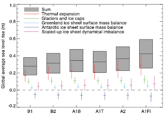
Figure 10.33. Projections and uncertainties (5 to 95% ranges) of global average sea level rise and its components in 2090 to 2099 (relative to 1980 to 1999 ) for the six SRES marker scenarios. The projected sea level rise assumes that the part of the present-day ice sheet mass imbalance that is due to recent ice flow acceleration will persist unchanged. It does not include the contribution shown from scaled-up ice sheet discharge, which is an alternative possibility. It is also possible that the present imbalance might be transient, in which case the projected sea level rise is reduced by 0.02 m. It must be emphasized that we cannot assess the likelihood of any of these three alternatives, which are presented as illustrative. The state of understanding prevents a best estimate from being made.
In all scenarios, the average rate of rise during the 21st century is very likely to exceed the 1961 to 2003 average rate of 1.8 ± 0.5 mm yr–1 (see Section 5.5.2.1 ). The central estimate of the rate of sea level rise during 2090 to 2099 is 3.8 mm yr–1 under A1B, which exceeds the central estimate of 3.1 mm yr–1 for 1993 to 2003 (see Section 5.5.2.2 ). The 1993 to 2003 rate may have a contribution of about 1 mm yr–1 from internally generated or naturally forced decadal variability (see Sections 5.5.2.4 and 9.5.2 ). These sources of variability are not predictable and not included in the projections; the actual rate during any future decade might therefore be more or less than the projected rate by a similar amount. Although simulated and observed sea level rise agree reasonably well for 1993 to 2003, the observed rise for 1961 to 2003 is not satisfactorily explained( Section 9.5.2 ), as the sum of observationally estimated components is 0.7 ± 0.7 mm yr–1 less than the observed rate of rise( Section 5.5.6 ). This indicates a deficiency in current scientific understanding of sea level change and may imply an underestimate in projections.
For an average model (the central estimate for each scenario), the scenario spread (from B1 to A1FI) in sea level rise is only 0.02 m by the middle of the century. This is small because of the time-integrating effect of sea level rise, on which the divergence among the scenarios has had little effect by then. By 2090 to 2099 it is 0.15 m.
In all scenarios, the central estimate for thermal expansion by the end of the century is 70 to 75% of the central estimate for the sea level rise. In all scenarios, the average rate of expansion during the 21st century is larger than central estimate of 1.6 mm yr–1 for 1993 to 2003 ( Section 5.5.3 ). Likewise, in all scenarios the average rate of mass loss by G&IC during the 21st century is greater than the central estimate of 0.77 mm yr–1 for 1993 to 2003 ( Section 4.5.2 ). By the end of the century, a large fraction of the present global G&IC mass is projected to have been lost (see, e.g., Table 4.3 ). The G&IC projections are rather insensitive to the scenario because the main uncertainties come from the G&IC model.
Further accelerations in ice flow of the kind recently observed in some Greenland outlet glaciers and West Antarctic ice streams could increase the ice sheet contributions substantially, but quantitative projections cannot be made with confidence (see Section 10.6.4.2 ). The land ice sum in Table 10.7 includes the effect of dynamical changes in the ice sheets that can be simulated with a continental ice sheet model( Section 10.6.4.2 ). It also includes a scenario-independent term of 0.32 ± 0.35 mm yr–1 (0.035 ± 0.039 m in 110 years). This is the central estimate for 1993 to 2003 of the sea level contribution from the Antarctic Ice Sheet, plus half of that from Greenland (Sections 4.6.2.2 and 5.5.5.2 ). We take this as an estimate of the part of the present ice sheet mass imbalance that is due to recent ice flow acceleration( Section 4.6.3.2 ), and assume that this contribution will persist unchanged.
We also evaluate the contribution of rapid dynamical changes under two alternative assumptions (see, e.g., Alley et al., 2005b [SRC] ). First, the present imbalance might be a rapid short-term adjustment, which will diminish during coming decades. We take an e-folding time of 100 years, on the basis of an idealised model study ( Payne et al., 2004 [JoC, SRC] ). This assumption reduces the sea level rise in Table 10.7 by 0.02 m. Second, the present imbalance might be a response to recent climate change, perhaps through oceanic or surface warming( Section 10.6.4.2 ). No models are available for such a link, so we assume that the imbalance might scale up with global average surface temperature change, which we take as a measure of the magnitude of climate change (see Appendix 10 .A). This assumption adds 0.1 to 0.2 m to the estimated upper bound for sea level rise depending on the scenario( Table 10.7 ). During 2090 to 2099, the rate of scaled-up antarctic discharge roughly balances the increased rate of antarctic accumulation (SMB). The central estimate for the increased antarctic discharge under the SRES scenario A1FI is about 1.3 mm yr–1,a factor of 5 to 10 greater than in recent years, and similar to the order-of-magnitude upper limit of Section 10.6.4.2 .It must be emphasized that we cannot assess the likelihood of any of these three alternatives, which are presented as illustrative. The state of understanding prevents a best estimate from being made.
The central estimates for sea level rise in Table 10.7 are smaller than the TAR model means ( Church et al., 2001 [NPR, ARC] ) by 0.03 to 0.07 m, depending on scenario, for two reasons. First, these projections are for 2090 - 2099, whereas the TAR projections were for 2100 . Second, the TAR included some small constant additional contributions to sea level rise which are omitted here (see below regarding permafrost). If the TAR model means are adjusted for this, they are within 10% of the central estimates from Table 10.7 .(See Appendix 10 .A for further information.) For each scenario, the upper bound of sea level rise in Table 10.7 is smaller than in the TAR, and the lower bound is larger than in the TAR. This is because the uncertainty on the sea level projection has been reduced, for a combination of reasons (see Appendix 10 .A for details). The TAR would have had similar ranges to those shown here if it had treated the uncertainties in the same way.
Thawing of permafrost is projected to contribute about 5 mm during the 21st century under the SRES scenario A2 (calculated from Lawrence and Slater, 2005 [JoC, MoS, SRC] ). The mass of the ocean will also be changed by climatically driven alteration in other water storage, in the forms of atmospheric water vapour, seasonal snow cover, soil moisture, groundwater, lakes and rivers. All of these are expected to be relatively small terms, but there may be substantial contributions from anthropogenic change in terrestrial water storage, through extraction from aquifers and impounding in reservoirs (see Sections 5.5.5.3 and 5.5.5.4 ).
10.7 Long Term Climate Change and Commitment
10.7.1 Climate Change Commitment to Year 2300 Based on AOGCMs
Building on Wigley 2005 [PoC, JoC, SRC] ), we use three specific definitions of climate change commitment: (i) the ‘constant composition commitment’, which denotes the further change of temperature (‘constant composition temperature commitment’ or ‘committed warming’), sea level (‘constant composition sea level commitment’) or any other quantity in the climate system, since the time the composition of the atmosphere, and hence the radiative forcing, has been held at a constant value; (ii) the ‘constant emission commitment’, which denotes the further change of, for example, temperature (‘constant emission temperature commitment’) since the time the greenhouse gas emissions have been held at a constant value; and (iii) the ‘zero emission commitment’, which denotes the further change of, for example, temperature (‘zero emission temperature commitment’) since the time the greenhouse gas emissions have been set to zero.
The concept that the climate system exhibits commitment when radiative forcing has changed is mainly due to the thermal inertia of the oceans, and was discussed independently by Wigley 1984 [PoC, JoC, SRC] Hansen et al. 1984 [NPR, SRC] and Siegenthaler and Oeschger 1984 [MoS] ). The term ‘commitment’ in this regard was introduced by Ramanathan 1988 [JoC, ARC] ). In the TAR, this was illustrated in idealised scenarios of doubling and quadrupling atmospheric CO2,and stabilisation at 2050 and 2100 after an IS92a forcing scenario. Various temperature commitment values were reported (about 0.3°C per century with much model dependency), and EMIC simulations were used to illustrate the long-term influence of the ocean owing to long mixing times and the MOC. Subsequent studies have confirmed this behaviour of the climate system and ascribed it to the inherent property of the climate system that the thermal inertia of the ocean introduces a lag to the warming of the climate system after concentrations of greenhouse gases are stabilised ( Mitchell et al., 2000 [JoC, SRC] ; Wetherald et al., 2001 [JoC, SRC] ; Wigley and Raper, 2003 [NPR, PoC, MoS, SRC] ; Hansen et al., 2005b [JoC, MoS, SRC] ; Meehl et al., 2005c [JoC, SRC] ; Wigley, 2005 [PoC, JoC, SRC] ). Climate change commitment as discussed here should not be confused with ‘unavoidable climate change’ over the next half century, which would surely be greater because forcing cannot be instantly stabilised. Furthermore, in the very long term it is plausible that climate change could be less than in a commitment run since forcing could plausibly be reduced below current levels as illustrated in the overshoot simulations and zero emission commitment simulations discussed below.
Three constant composition commitment experiments have recently been performed by the global coupled climate modelling community: (1) stabilising concentrations of greenhouse gases at year 2000 values after a 20th-century climate simulation, and running the model for an additional 100 years; (2) stabilising concentrations of greenhouse gases at year 2100 values after a 21st-century B1 experiment (e.g., CO2 near 550 ppm) and running the model for an additional 100 years (with some models run to 200 years); and (3) stabilising concentrations of greenhouse gases at year 2100 values after a 21st-century A1B experiment (e.g., CO2 near 700 ppm), and running the model for an additional 100 years (and some models to 200 years). Multi-model mean warming in these experiments is depicted in Figure 10.4 .Time series of the globally averaged surface temperature and percent precipitation change after stabilisation are shown for all the models in the Supplementary Material, Figure S10.3.
The multi-model average warming for all radiative forcing agents held constant at year 2000 (reported earlier for several of the models by Meehl et al., 2005c [JoC, SRC] ), is about 0.6°C for the period 2090 to 2099 relative to the 1980 to 1999 reference period. This is roughly the magnitude of warming simulated in the 20th century. Applying the same uncertainty assessment as for the SRES scenarios in Fig. 10.29 (–40 to +60%), the likely uncertainty range is 0.3°C to 0.9°C. Hansen et al. 2005a [JoC, SRC] ) calculate the current energy imbalance of the Earth to be 0.85 Wm–2,implying that the unrealised global warming is about 0.6°C without any further increase in radiative forcing. The committed warming trend values show a rate of warming averaged over the first two decades of the 21st century of about 0.1°C per decade, due mainly to the slow response of the oceans. About twice as much warming (0.2°C per decade) would be expected if emissions are within the range of the SRES scenarios.
For the B1 constant composition commitment run, the additional warming after 100 years is also about 0.5°C, and roughly the same for the A1B constant composition commitment (Supplementary Material, Figure S10.3). These new results quantify what was postulated in the TAR in that the warming commitment after stabilising concentrations is about 0.5°C for the first century, and considerably smaller after that, with most of the warming commitment occurring in the first several decades of the 22nd century.
Constant composition precipitation commitment for the multi-model ensemble average is about 1.1% by 2100 for the 20th-century constant composition commitment experiment, and for the B1 constant composition commitment experiment it is 0.8% by 2200 and 1.5% by 2300, while for the A1B constant composition commitment experiment it is 1.5% by 2200 and 2% by 2300 .
The patterns of change in temperature in the B1 and A1B experiments, relative to the pre-industrial period, do not change greatly after stabilisation( Table 10.5 ). Even the 20th-century stabilisation case warms with some similarity to the A1B pattern( Table 10.5 ). However, there is some contrast in the land and ocean warming rates, as seen from Figure 10.6 .Mid- and low-latitude land warms at rates closer to the global mean of that of A1B, while high-latitude ocean warming is larger.
10.7.2 Climate Change Commitment to Year 3000 and Beyond to Equilibrium
Earth System Models of Intermediate Complexity are used to extend the projections for a scenario that follows A1B to 2100 and then keeps atmospheric composition, and hence radiative forcing, constant to the year 3000 (see Figure 10.34 ). By 2100, the projected warming is between 1.2°C and 4.1°C, similar to the range projected by AOGCMs. A large constant composition temperature and sea level commitment is evident in the simulations and is slowly realised over coming centuries. By the year 3000, the warming range is 1.9°C to 5.6°C. While surface temperatures approach equilibrium relatively quickly, sea level continues to rise for many centuries.
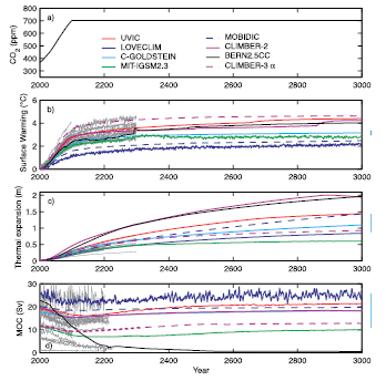
Figure 10.34. (a) Atmospheric CO2,(b) global mean surface warming, (c) sea level rise from thermal expansion and (d) Atlantic meridional overturning circulation (MOC) calculated by eight EMICs for the SRES A1B scenario and stable radiative forcing after 2100, showing long-term commitment after stabilisation. Coloured lines are results from EMICs, grey lines indicate AOGCM results where available for comparison. Anomalies in (b) and (c) are given relative to the year 2000 . Vertical bars indicate ±2 standard deviation uncertainties due to ocean parameter perturbations in the C-GOLDSTEIN model. The MOC shuts down in the BERN2.5CC model, leading to an additional contribution to sea level rise. Individual EMICs (see Table 8.3 for model details) treat the effect from non-CO2 greenhouse gases and the direct and indirect aerosol effects on radiative forcing differently. Despite similar atmospheric CO2 concentrations, radiative forcing among EMICs can thus differ within the uncertainty ranges currently available for present-day radiative forcing (see Chapter2 ).
Five of these EMICs include interactive representations of the marine and terrestrial carbon cycle and, therefore, can be used to assess carbon cycle-climate feedbacks and effects of carbon emission reductions on atmospheric CO2 and climate. Although carbon cycle processes in these models are simplified, global-scale quantities are in good agreement with more complex models ( Doney et al., 2004 [JoC, MoS] ).
Results for one carbon emission scenario are shown in Figure 10.35 ,where anthropogenic emissions follow a path towards stabilisation of atmospheric CO2 at 750 ppm but at year 2100 are reduced to zero. This permits the determination of the zero emission climate change commitment. The prescribed emissions were calculated from the SP750 profile ( Knutti et al., 2005 [JoC, MoS, SRC] ) using the BERN-CC model ( Joos et al., 2001 [PoC, JoC, SRC] ). Although unrealistic, such a scenario permits the calculation of zero emission commitment, i.e., climate change due to 21st-century emissions. Even though emissions are instantly reduced to zero at year 2100, it takes about 100 to 400 years in the different models for the atmospheric CO2 concentration to drop from the maximum (ranges between 650 to 700 ppm) to below the level of doubled pre-industrial CO2 (~560 ppm) owing to a continuous transfer of carbon from the atmosphere into the terrestrial and oceanic reservoirs. Emissions during the 21st century continue to have an impact even at year 3000 when both surface temperature and sea level rise due to thermal expansion are still substantially higher than pre-industrial. Also shown are atmospheric CO2 concentrations and ocean/terrestrial carbon inventories at year 3000 versus total emitted carbon for similar emission pathways targeting (but not actually reaching) 450, 550, 750 and 1,000 ppm atmospheric CO2 and with carbon emissions reduced to zero at year 2100 . Atmospheric CO2 at year 3000 is approximately linearly related to the total amount of carbon emitted in each model, but with a substantial spread among the models in both slope and absolute values, because the redistribution of carbon between the different reservoirs is model dependent. In summary, the model results show that 21st-century emissions represent a minimum commitment of climate change for several centuries, irrespective of later emissions. A reduction of this ‘minimum’ commitment is possible only if, in addition to avoiding CO2 emissions after 2100, CO2 were actively removed from the atmosphere.
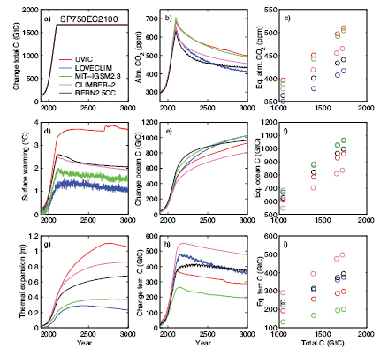
Figure 10.35. Changes in carbon inventories and climate response relative to the pre-industrial period simulated by five different intermediate complexity models (see Table 8.3 for model descriptions) for a scenario where emissions follow a pathway leading to stabilisation of atmospheric CO2 at 750 ppm, but before reaching this target, emissions are reduced to zero instantly at year 2100 . (a) Change in total carbon, (b) atmospheric CO2,(d) change in surface temperature, (e) change in ocean carbon, (g) sea level rise from thermal expansion and (h) change in terrestrial carbon. Right column: (c) atmospheric CO2 and the change in (f) oceanic and (i) terrestrial carbon inventories at year 3000 relative to the pre-industrial period for several emission scenarios of similar shape but with different total carbon emissions.
Using a similar approach, Friedlingstein and Solomon 2005 [PoC, JoC, SRC] ) show that even if emissions were immediately cut to zero, the system would continue to warm for several more decades before starting to cool. It is important also to note that ocean heat content and changes in the cryosphere evolve on time scales extending over centuries.
On very long time scales (order several thousand years as estimated by AOGCM experiments, Bi et al., 2001 [JoC, MoS] ; Stouffer, 2004 [JoC, SRC] ), equilibrium climate sensitivity is a useful concept to characterise the ultimate response of climate models to different future levels of greenhouse gas radiative forcing. This concept can be applied to climate models irrespective of their complexity. Based on a global energy balance argument, equilibrium climate sensitivity S and global mean surface temperature increase ΔT at equilibrium relative to pre-industrial for an equivalent stable CO2 concentration are linearly related according to ΔT = S × log(CO2 / 280 ppm) / log(2), which follows from the definition of climate sensitivity and simplified expressions for the radiative forcing of CO2 (Section 6.3.5 of the TAR). Because the combination of various lines of modelling results and expert judgement yields a quantified range of climate sensitivity S (see Box 10.2 ), this can be carried over to equilibrium temperature increase. Most likely values, and the likely range, as well as a very likely lower bound for the warming, all consistent with the quantified range of S,are given in Table 10.8 .
Table 10.8. Best guess (i.e. most likely), likely and very likely bounds/ranges of global mean equilibrium surface temperature increase DT(°C) above pre-industrial temperatures for different levels of CO2 equivalent concentrations (ppm), based on the assessment of climate sensitivity given in Box 10.2 .
| Equivalent CO2 | Best Guess | Very Likely Above | Likely inthe Range |
|---|---|---|---|
| 350 | 1.0 | 0.5 | 0.6–1.4 |
| 450 | 2.1 | 1.0 | 1.4–3.1 |
| 550 | 2.9 | 1.5 | 1.9–4.4 |
| 650 | 3.6 | 1.8 | 2.4–5.5 |
| 750 | 4.3 | 2.1 | 2.8–6.4 |
| 1,000 | 5.5 | 2.8 | 3.7–8.3 |
| 1,200 | 6.3 | 3.1 | 4.2–9.4 |
It is emphasized that this table does not contain more information than the best knowledge of S and that the numbers are not the result of any climate model simulation. Rather it is assumed that the above relationship between temperature increase and CO2 holds true for the entire range of equivalent CO2 concentrations. There are limitations to the concept of radiative forcing and climate sensitivity ( Senior and Mitchell, 2000 [JoC, ARC] ; Joshi et al., 2003 [JoC, MoS] ; Shine et al., 2003 [JoC, MoS] ; Hansen et al., 2005b [JoC, MoS, SRC] ). Only a few AOGCMs have been run to equilibrium under elevated CO2 concentrations, and some results show that nonlinearities in the feedbacks (e.g., clouds, sea ice and snow cover) may cause a time dependence of the effective climate sensitivity and substantial deviations from the linear relation assumed above ( Manabe and Stouffer, 1994 [JoC, MoS, SRC] ; Senior and Mitchell, 2000 [JoC, ARC] ; Voss and Mikolajewicz, 2001 [JoC, MoS] ; Gregory et al., 2004b [JoC, MoS, SRC] ), with effective climate sensitivity tending to grow with time in some of the AR4 AOGCMs. Some studies suggest that climate sensitivities larger than the likely estimate given below (which would suggest greater warming) cannot be ruled out (see Box 10.2 on climate sensitivity).
Another way to address eventual equilibrium temperature for different CO2 concentrations is to use the projections from the AOGCMs in Figure 10.4 ,and an idealised 1% yr–1 CO2 increase to 4 × CO2.The equivalent CO2 concentrations in the AOGCMs can be estimated from the forcings given in Table 6.14 in the TAR. The actual CO2 concentrations for A1B and B1 are roughly 715 ppm and 550 ppm (depending on which model is used to convert emissions to concentrations), and equivalent CO2 concentrations are estimated to be about 835 ppm and 590 ppm, respectively. Using the equation above for an equilibrium climate sensitivity of 3.0°C, eventual equilibrium warming in these experiments would be 4.8°C and 3.3°C, respectively. The multi-model average warming in the AOGCMs at the end of the 21st century (relative to pre-industrial temperature) is 3.1°C and 2.3°C, or about 65 to 70% of the eventual estimated equilibrium warming. Given rates of CO2 increase of between 0.5 and 1.0% yr–1 in these two scenarios, this can be compared to the calculated fraction of eventual warming of around 50% in AOGCM experiments with those CO2 increase rates ( Stouffer and Manabe, 1999 [JoC, MoS, SRC] ). The Stouffer and Manabe 1999 [JoC, MoS, SRC] ) model has somewhat higher equilibrium climate sensitivity, and was actually run to equilibrium in a 4-kyr integration to enable comparison of transient and equilibrium warming. Therefore, the AOGCM results combined with the estimated equilibrium warming seem roughly consistent with earlier AOGCM experiments of transient warming rates. Additionally, similar numbers for the 4 × CO2 stabilisation experiments performed with the AOGCMs can be computed. In that case, the actual and equivalent CO2 concentrations are the same, since there are no other radiatively active species changing in the models, and the multi-model CO2 concentration at quadrupling would produce an eventual equilibrium warming of 6°C, where the multi-model average warming at the time of quadrupling is about 4.0°C or 66% of eventual equilibrium. This is consistent with the numbers for the A1B and B1 scenario integrations with the AOGCMs.
It can be estimated how much closer to equilibrium the climate system is 100 years after stabilisation in these AOGCM experiments. After 100 years of stabilised concentrations, the warming relative to pre-industrial temperature is 3.8°C in A1B and 2.6°C in B1, or about 80% of the estimated equilibrium warming. For the stabilised 4 × CO2 experiment, after 100 years of stabilised CO2 concentrations the warming is 4.7°C, or 78% of the estimated equilibrium warming. Therefore, about an additional 10 to 15% of the eventual equilibrium warming is achieved after 100 years of stabilised concentrations ( Stouffer, 2004 [JoC, SRC] ). This emphasizes that the approach to equilibrium takes a long time, and even after 100 years of stabilised atmospheric concentrations, only about 80% of the eventual equilibrium warming is realised.
10.7.3 Long-Term Integrations: Idealised Overshoot Experiments
The concept of mitigation related to overshoot scenarios has implications for IPCC Working Groups II and III and was addressed in the Second Assessment Report. A new suite of mitigation scenarios is currently being assessed for the AR4. Working Group I does not have the expertise to assess such scenarios, so this section assesses the processes and response of the physical climate system in a very idealised overshoot experiment. Plausible new mitigation and overshoot scenarios will be run subsequently by modelling groups and assessed in the next IPCC report.
An idealised overshoot scenario has been run in an AOGCM where the CO2 concentration decreases from the A1B stabilised level to the B1 stabilised level between 2150 and 2250, followed by 200 years of integration with that constant B1 level( Figure 10.36 a). This reduction in CO2 concentration would require large reductions in emissions, but such an idealised experiment illustrates the processes involved in how the climate system would respond to such a large change in emissions and concentrations. Yoshida et al. 2005 [MoS] and Tsutsui et al. 2007 [JoC, MoS, 2007] ) show that there is a relatively fast response in the surface and upper ocean, which start to recover to temperatures at the B1 level after several decades, but a much more sluggish response with more commitment in the deep ocean. As shown in Figure 10.36 band c, the overshoot scenario temperatures only slowly decrease to approach the lower temperatures of the B1 experiment, and continue a slow convergence that has still not cooled to the B1 level at the year 2350, or 100 years after the CO2 concentration in the overshoot experiment was reduced to equal the concentration in the B1 experiment. However, Dai et al. 2001a [PoC, JoC, SRC] ) show that reducing emissions to achieve a stabilised CO2 concentration in the 21st century reduces warming moderately (less than 0.5°C) by the end of the 21st century in comparison to a business-as-usual scenario, but the warming reduction is about 1.5°C by the end of the 22nd century in that experiment. Other climate system responses include the North Atlantic MOC and sea ice volume that almost recover to the B1 level in the overshoot scenario experiment, except for a significant hysteresis effect that is shown in the sea level change due to thermal expansion ( Yoshida et al., 2005 [MoS] ; Nakashiki et al., 2006 [JoC] ).
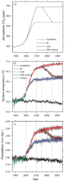
Figure 10.36. (a) Atmospheric CO2 concentrations for several experiments simulated with an AOGCM; (b) globally averaged surface air temperatures for the overshoot scenario and the A1B and B1 experiments; (c) same as in (b) but for globally averaged precipitation rate. Modified from Yoshida et al. 2005 [MoS] ).
Such stabilisation and overshoot scenarios have implications for risk assessment as suggested by Yoshida et al. 2005 [MoS] ) and others. For example, in a probabilistic study using an SCM and multi-gas scenarios, Meinshausen 2006 [NPR, MoS, SRC] ) estimated that the probability of exceeding a 2°C warming is between 68 and 99% for a stabilisation of equivalent CO2 at 550 ppm. They also considered scenarios with peaking CO2 and subsequent stabilisation at lower levels as an alternative pathway and found that if the risk of exceeding a warming of 2°C is not to be greater than 30%, it is necessary to peak equivalent CO2 concentrations around 475 ppm before returning to lower concentrations of about 400 ppm. These overshoot and targeted climate change estimations take into account the climate change commitment in the system that must be overcome on the time scale of any overshoot or emissions target calculation. The probabilistic studies also show that when certain thresholds of climate change are to be avoided, emission pathways depend on the certainty requested of not exceeding the threshold.
Earth System Models of Intermediate Complexity have been used to calculate the long-term climate response to stabilisation of atmospheric CO2,although EMICs have not been adjusted to take into account the full range of AOGCM sensitivities. The newly developed stabilisation profiles were constructed following Enting et al. 1994 [NPR, PoC, MoS, SRC] and Wigley et al. 1996 [PoC, JoC, SRC] ) using the most recent atmospheric CO2 observations, CO2 projections with the BERN-CC model ( Joos et al., 2001 [PoC, JoC, SRC] ) for the A1T scenario over the next few decades, and a ratio of two polynomials ( Enting et al., 1994 [NPR, PoC, MoS, SRC] ) leading to stabilisation at levels of 450, 550, 650, 750 and 1,000 ppm atmospheric CO2 equivalent. Other forcings are not considered. Supplementary Material, Figure S10.4a shows the equilibrium surface warming for seven different EMICs and six stabilisation levels. Model differences arise mainly from the models having different climate sensitivities.
Knutti et al. 2005 [JoC, MoS, SRC] ) explore this further with an EMIC using several published PDFs of climate sensitivity and different ocean heat uptake parametrizations and calculate probabilities of not overshooting a certain temperature threshold given an equivalent CO2 stabilisation level (Supplementary Material, Figure S10.4b). This plot illustrates, for example, that for low values of stabilised CO2,the range of response of possible warming is smaller than for high values of stabilised CO2.This is because with greater CO2 forcing, there is a greater spread of outcomes as illustrated in Figure 10.26 .Figure S10.4b also shows that for any given temperature threshold, the smaller the desired probability of exceeding the target is, the lower the stabilisation level that must be chosen. Stabilisation of atmospheric greenhouse gases below about 400 ppm CO2 equivalent is required to keep the global temperature increase likely less than 2°C above pre-industrial temperature ( Knutti et al., 2005 [JoC, MoS, SRC] ).
10.7.4 Commitment to Sea Level Rise
10.7.4.1 Thermal Expansion
The sea level rise commitment due to thermal expansion has much longer time scales than the surface warming commitment, owing to the slow processes that mix heat into the deep ocean ( Church et al., 2001 [NPR, ARC] ). If atmospheric composition were stabilised at A1B levels in 2100, thermal expansion in the 22nd century would be similar to in the 21st (see, e.g., Section 10.6.1 ;Meehl et al., 2005c [JoC, SRC] ), reaching 0.3 to 0.8 m by 2300 ( Figure 10.37 ). The ranges of thermal expansion overlap substantially for stabilisation at different levels, since model uncertainty is dominant; A1B is given here because results are available from more models for this scenario than for other scenarios. Thermal expansion would continue over many centuries at a gradually decreasing rate( Figure 10.34 ). There is a wide spread among the models for the thermal expansion commitment at constant composition due partly to climate sensitivity, and partly to differences in the parametrization of vertical mixing affecting ocean heat uptake (e.g., Weaver and Wiebe, 1999 [JoC, SRC] ). If there is deep-water formation in the final steady state as in the present day, the ocean will eventually warm up fairly uniformly by the amount of the global average surface temperature change ( Stouffer and Manabe, 2003 [JoC, SRC] ), which would result in about 0.5 m of thermal expansion per degree celsius of warming, calculated from observed climatology; the EMICs in Figure 10.34 indicate 0.2 to 0.6 m °C–1 for their final steady state (year 3000) relative to 2000 . If deep-water formation is weakened or suppressed, the deep ocean will warm up more ( Knutti and Stocker, 2000 [JoC, SRC] ). For instance, in the 3 × CO2 experiment of Bi et al. 2001 [JoC, MoS] ) with the CSIRO AOGCM, both North Atlantic Deep Water and Antarctic Bottom Water formation cease, and the steady-state thermal expansion is 4.5 m. Although these commitments to sea level rise are large compared with 21st-century changes, the eventual contributions from the ice sheets could be larger still.
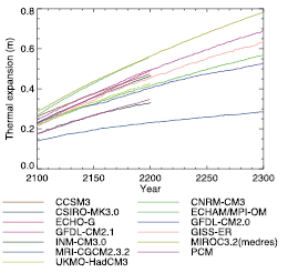
Figure 10.37. Globally averaged sea level rise from thermal expansion relative to the period 1980 to 1999 for the A1B commitment experiment calculated from AOGCMs. See Table 8.1 for model details.
10.7.4.2 Glaciers and Ice Caps
Steady-state projections for G&IC require a model that evolves their area-altitude distribution (see, e.g., Section 10.6.3.3 ). Little information is available on this. A comparative study including seven GCM simulations at 2 × CO2 conditions inferred that many glaciers may disappear completely due to an increase of the equilibrium line altitude ( Bradley et al., 2004 [PoC, JoC] ), but even in a warmer climate, some glacier volume may persist at high altitude. With a geographically uniform warming relative to 1900 of 4°C maintained after 2100, about 60% of G&IC volume would vanish by 2200 and practically all by 3000 ( Raper and Braithwaite, 2006 [JoC, MoS, SRC] ). Nonetheless, this commitment to sea level rise is relatively small (<1 m; Table 4.4 )compared with those from thermal expansion and ice sheets.
10.7.4.3 Greenland Ice Sheet
The present SMB of Greenland is a net accumulation estimated as 0.6 mm yr–1 of sea level equivalent from a compilation of studies ( Church et al., 2001 [NPR, ARC] ) and 0.47 mm yr–1 for 1988 to 2004 ( Box et al., 2006 [JoC, ARC] ). In a steady state, the net accumulation would be balanced by calving of icebergs. General Circulation Models suggest that ablation increases more rapidly than accumulation with temperature ( van de Wal et al., 2001 [Ambiguous] ; Gregory and Huybrechts, 2006 [JoC, MoS, SRC] ), so warming will tend to reduce the SMB, as has been observed in recent years (see Section 4.6.3 ), and is projected for the 21st century( Section 10.6.4.1 ). Sufficient warming will reduce the SMB to zero. This gives a threshold for the long-term viability of the ice sheet because negative SMB means that the ice sheet must contract even if ice discharge has ceased owing to retreat from the coast. If a warmer climate is maintained, the ice sheet will eventually be eliminated, except perhaps for remnant glaciers in the mountains, raising sea level by about 7 m (see Table 4.1 Huybrechts et al. 1991 [SRC] ) evaluated the threshold as 2.7°C of seasonally and geographically uniform warming over Greenland relative to a steady state (i.e. pre-industrial temperature). Gregory et al. 2004a [JoC, SRC] ) examine the probability of this threshold being reached under various CO2 stabilisation scenarios for 450 to 1000 ppm using TAR projections, and find that it was exceeded in 34 out of 35 combinations of AOGCM and CO2 concentration considering seasonally uniform warming, and 24 out of 35 considering summer warming and using an upper bound on the threshold.
Assuming the warming to be uniform underestimates the threshold, because warming is projected by GCMs to be weaker in the ablation area and in summer, when ablation occurs. Using geographical and seasonal patterns of simulated temperature change derived from a combination of four high-resolution AGCM simulations and 18 AR4 AOGCMs raises the threshold to 3.2°C to 6.2°C in annual- and area-average warming in Greenland, and 1.9°C to 4.6°C in the global average ( Gregory and Huybrechts, 2006 [JoC, MoS, SRC] ), relative to pre-industrial temperatures. This is likely to be reached by 2100 under the SRES A1B scenario, for instance( Figure 10.29 ). These results are supported by evidence from the last interglacial, when the temperature in Greenland was 3°C to 5°C warmer than today and the ice sheet survived, but may have been smaller by 2 to 4 m in sea level equivalent (including contributions from arctic ice caps, see Section 6.4.3 ). However, a lower threshold of 1°C ( Hansen, 2005 [JoC, SRC] ) in global warming above present-day temperatures has also been suggested, on the basis that global mean (rather than Greenland) temperatures during previous interglacials exceeded today’s temperatures by no more than that.
For stabilisation in 2100 with SRES A1B atmospheric composition, Greenland would initially contribute 0.3 to 2.1 mm yr–1 to sea level( Table 10.7 ). The greater the warming, the faster the loss of mass. Ablation would be further enhanced by the lowering of the surface, which is not included in the calculations in Table 10.7 .To include this and other climate feedbacks in calculating long-term rates of sea level rise requires coupling an ice sheet model to a climate model. Ridley et al. 2005 [JoC, SRC] ) couple the Greenland Ice Sheet model of Huybrechts and de Wolde 1999 [JoC, SRC] ) to the UKMO-HadCM3 AOGCM. Under constant 4 × CO2,the sea level contribution is 5.5 mm yr–1 over the first 300 years and declines as the ice sheet contracts; after 1 kyr only about 40% of the original volume remains and after 3 kyr only 4%( Figure 10.38 ). The rate of deglaciation would increase if ice flow accelerated, as in recent years( Section 4.6.3.3 ). Basal lubrication due to surface melt water might cause such an effect (see Section 10.6.4.2 ). The best estimate of Parizek and Alley 2004 [JoC, MoS, SRC] ) is that this could add an extra 0.15 to 0.40 m to sea level by 2500, compared with 0.4 to 3.2 m calculated by Huybrechts and de Wolde 1999 [JoC, SRC] ) without this effect. The processes whereby melt water might penetrate through subfreezing ice to the bed are unclear and only conceptual models exist at present ( Alley et al., 2005b [SRC] ).
Under pre-industrial or present-day atmospheric CO2 concentrations, the climate of Greenland would be much warmer without the ice sheet, because of lower surface altitude and albedo, so it is possible that Greenland deglaciation and the resulting sea level rise would be irreversible. Toniazzo et al. 2004 [JoC, SRC] ) find that snow does not accumulate anywhere on an ice-free Greenland with pre-industrial atmospheric CO2,whereas Lunt et al. 2004 [JoC] ) obtain a substantial regenerated ice sheet in east and central Greenland using a higher-resolution model.
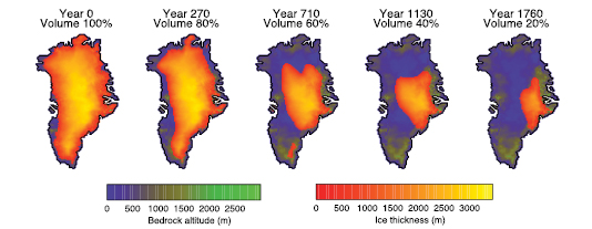
Figure 10.38. Evolution of Greenland surface elevation and ice sheet volume versus time in the experiment of Ridley et al. 2005 [JoC, SRC] ) with the UKMO-HadCM3 AOGCM coupled to the Greenland Ice Sheet model of Huybrechts and de Wolde 1999 [JoC, SRC] ) under a climate of constant quadrupled pre-industrial atmospheric CO2.
10.7.4.4 Antarctic Ice Sheet
With rising global temperature, GCMs indicate increasingly positive SMB for the Antarctic Ice Sheet as a whole because of greater accumulation( Section 10.6.4.1 ). For stabilisation in 2100 with SRES A1B atmospheric composition, antarctic SMB would contribute 0.4 to 2.0 mm yr–1 of sea level fall( Table 10.7 ). Continental ice sheet models indicate that this would be offset by tens of percent by increased ice discharge( Section 10.6.4.2 ), but still give a negative contribution to sea level, of –0.8 m by 3000 in one simulation with antarctic warming of about 4.5°C ( Huybrechts and de Wolde, 1999 [JoC, SRC] ).
However, discharge could increase substantially if buttressing due to the major West Antarctic ice shelves were reduced (see Sections 4.6.3.3 and 10.6.4.2 ), and could outweigh the accumulation increase, leading to a net positive antarctic sea level contribution in the long term. If the Amundsen Sea sector were eventually deglaciated, it would add about 1.5 m to sea level, while the entire West Antarctic Ice Sheet (WAIS) would account for about 5 m ( Vaughan, 2007 [NPR, JoC, SRC, 2007] ). Contributions could also come in this manner from the limited marine-based portions of East Antarctica that discharge into large ice shelves.
Weakening or collapse of the ice shelves could be caused either by surface melting or by thinning due to basal melting. In equilibrium experiments with mixed-layer ocean models, the ratio of antarctic to global annual warming is 1.4 ± 0.3. Following reasoning in Section 10.6.4.2 and Appendix 10 .A, it appears that mean summer temperatures over the major West Antarctic ice shelves are about as likely as not to pass the melting point if global warming exceeds 5°C, and disintegration might be initiated earlier by surface melting. Observational and modelling studies indicate that basal melt rates depend on water temperature near to the base, with a constant of proportionality of about 10 m yr–1 °C–1 indicated for the Amundsen Sea ice shelves ( Rignot and Jacobs, 2002 [JoC, ARC] ; Shepherd et al., 2004 [JoC, SRC] ) and 0.5 to 10 m yr–1 °C–1 for the Amery ice shelf ( Williams et al., 2002 [JoC] ). If this order of magnitude applies to future changes, a warming of about 1°C under the major ice shelves would eliminate them within centuries. We are not able to relate this quantitatively to global warming with any confidence, because the issue has so far received little attention, and current models may be inadequate to treat it because of limited resolution and poorly understood processes. Nonetheless, it is reasonable to suppose that sustained global warming would eventually lead to warming in the seawater circulating beneath the ice shelves.
Because the available models do not include all relevant processes, there is much uncertainty and no consensus about what dynamical changes could occur in the Antarctic Ice Sheet (see, e.g., Vaughan and Spouge, 2002 [JoC, MoS, SRC] ; Alley et al., 2005a [JoC, SRC] ). One line of argument is to consider an analogy with palaeoclimate (see Box 4.1 ). Palaeoclimatic evidence that sea level was 4 to 6 m above present during the last interglacial may not all be explained by reduction in the Greenland Ice Sheet, implying a contribution from the Antarctic Ice Sheet (see Section 6.4.3 ). On this basis, using the limited available evidence, sustained global warming of 2°C ( Oppenheimer and Alley, 2005 [JoC, SRC] ) above present-day temperatures has been suggested as a threshold beyond which there will be a commitment to a large sea level contribution from the WAIS. The maximum rates of sea level rise during previous glacial terminations were of the order of 10 mm yr–1 ( Church et al., 2001 [NPR, ARC] ). We can be confident that future accelerated discharge from WAIS will not exceed this size, which is roughly an order of magnitude increase in present-day WAIS discharge, since no observed recent acceleration has exceeded a factor of ten.
Another line of argument is that there is insufficient evidence that rates of dynamical discharge of this magnitude could be sustained over long periods. The WAIS is 20 times smaller than the LGM NH ice sheets that contributed most of the melt water during the last deglaciation at rates that can be explained by surface melting alone ( Zweck and Huybrechts, 2005 [JoC, MoS, SRC] ). In the study of Huybrechts and de Wolde 1999 [JoC, SRC] ), the largest simulated rate of sea level rise from the Antarctic Ice Sheet over the next 1 kyr is 2.5 mm yr–1.This is dominated by dynamical discharge associated with grounding line retreat. The model did not simulate ice streams, for which widespread acceleration would give larger rates. However, the maximum loss of ice possible from rapid discharge of existing ice streams is the volume in excess of flotation in the regions occupied by these ice streams (defined as regions of flow exceeding 100 m yr–1;see Section 10.6.4.2 ). This volume (in both West and East Antarctica) is 230,000 km3,equivalent to about 0.6 m of sea level, or about 1% of the mass of the Antarctic Ice Sheet, most of which does not flow in ice streams. Loss of ice affecting larger portions of the ice sheet could be sustained at rapid rates only if new ice streams developed in currently slow-moving ice. The possible extent and rate of such changes cannot presently be estimated, since there is only very limited understanding of controls on the development and variability of ice streams. In this argument, rapid discharge may be transient and the long-term sign of the antarctic contribution to sea level depends on whether increased accumulation is more important than large-scale retreat of the grounding line.
10.A.1 Scaling MAGICC Results
The MAGICC SCM was tuned to emulate global average surface air temperature change and radiative flux at the top of the atmosphere (assumed equal to ocean heat uptake on decadal time scales; Section 5.2.2.3 and Figure 5.4 )simulated by each of 19 AOGCMs in scenarios with CO2 increasing at 1% yr–1 ( Section 10.5.3 ). Under SRES scenarios for which AOGCMs have been run (B1, A1B and A2), the ensemble average of the tuned versions of MAGICC gives about 10% greater temperature rise and 25% more thermal expansion over the 21st century ( 2090 to 2099 minus 1980 to 1999 ) than the average of the corresponding AOGCMs. The MAGICC radiative forcing is close to that of the AOGCMs (as estimated for A1B by Forster and Taylor, 2006 [JoC, MoS, SRC] ), so the mismatch suggests there may be structural limitations on the accurate emulation of AOGCMs by the SCM. We therefore do not use the tuned SCM results directly to make projections, unlike in the TAR. The TAR model means for thermal expansion were 0.06–0.10 m larger than the central estimates in Table 10.7 ,probably because the simple climate model used in the TAR overestimated the TAR AOGCM results.
The SCM may nonetheless be used to estimate results for scenarios that have not been run in AOGCMs, by calculating time-dependent ratios between pairs of scenarios( Section 10.5.4.6 ). This procedure is supported by the close match between the ratios derived from the AOGCM and MAGICC ensemble averages under the scenarios for which AOGCMs are available. Applying the MAGICC ratios to the A1B AOGCM results yields estimates of temperature rise and thermal expansion for B1 and A2 differing by less than 5% from the AOGCM ensemble averages. We have high confidence that the procedure will yield similarly accurate estimates for the results that the AOGCMs would give under scenarios B2, A1T and A1FI.
10.A.2 Mass Balance Sensitivity of Glaciers and Ice Caps
Alinear relationship rg= bg ×(T − T0)is found for the period 1961 to 2003 between the observational time series of the contribution rg to the rate of sea level rise from the world’s glaciers and ice caps (G&IC, excluding those on Antarctica and Greenland; Section 4.5.2 , Figure 4.14 )and global average surface air temperature T (Hadley Centre/Climatic Research Unit gridded surface temperature dataset HadCRUT3; Section 3.2.2.4 , Figure 3.6 ), where bg is the global total G&IC mass balance sensitivity and T0 is the global average temperature of the climate in which G&IC are in a steady state, T and T0 being expressed relative to the average of 1865 to 1894 . The correlation coefficient is 0.88. Weighted least-squares regression gives a slope bg = 0.84 ± 0.15 (one standard deviation) mm yr–1 °C–1,with T0=−0.13°C. Surface mass balance models driven with climate change scenarios from AOGCMs( Section 10.6.3.1 )also indicate such a linear relationship, but the model results give a somewhat lower bg of around 0.5 to 0.6 mm yr–1 °C–1 ( Section 10.6.3.1 ). To cover both observations and models, we adopt a value of bg = 0.8 ± 0.2 (one standard deviation) mm yr–1 °C–1.This uncertainty of ±25% is smaller than that of ±40% used in the TAR because of the improved observational constraint now available. To make projections, we choose a set of values of bg randomly from a normal distribution. We use T0 = T - rg/bg , where T =0.40 °C and rg =0.45 mm yr–1,are the averages over the period 1961 to 2003 . This choice of T0 minimises the root mean square difference of the predicted rg from the observed, and gives T0 in the range −0.5°C to 0.0°C (5 to 95%). Note that a constant bgis not expected to be a good approximation if glacier area changes substantially (see Section 10.A.3).
Model results using area-volume scaling of G&IC( Section 10.6.3.2 )are approximately described by the relations bg / b1 =(Ag / A1)1.96 and Ag / A1 =(Vg / V1)0.84,where Ag and Vg are the global G&IC area and volume (excluding those on Greenland and Antarctica) and variable X1is the initial value of Xg.The first relation describes how total SMB sensitivity declines as the most sensitive areas are ablated most rapidly. The second relation follows Wigley and Raper 2005 [PoC, JoC, MoS, SRC] ) in its form, and describes how area declines as volume is lost, withdVg /dt = −rg (expressing V as sea level equivalent, i.e., the liquid-water-equivalent volume of ice divided by the surface area of the world ocean). Projections are made starting from 1990 using T from Section 10.A.1 with initial values of the present-day bgfrom Section 10.A.2 and the three recent estimates Vg=0.15, 0.24 and 0.37 m from Table 4.4 ,which are assumed equally likely. We use T =0.48°C at 1990 relative to 1865 to 1894, and choose T0 as in Section 10.A.2. An uncertainty of 10% (one standard deviation) is assumed because of the scaling relations. The results are multiplied by 1.2( Section 10.6.3.3 )to include contributions from G&IC on Greenland and Antarctica (apart from the ice sheets). These scaling relations are expected to give a decreasingly adequate approximation as greater area and volume is lost, because they do not model hypsometry explicitly; they predict that V will tend eventually to zero in any steady-state warmer climate, for instance, although this is not necessarily the case. A similar scaling procedure was used in the TAR. Current estimates of present-day G&IC mass are smaller than those used in the TAR, leading to more rapid wastage of area. Hence, the central estimates for the G&IC contribution to sea level rise in Table 10.7 are similar to those in the TAR, despite our use of a larger mass balance sensitivity (Section 10.A.2).
10.A.4 Changes in Ice Sheet Surface Mass Balance
Quadratic fits are made to the results of Gregory and Huybrechts 2006 [JoC, MoS, SRC] )( Section 10.6.4.1 )for the SMB change of each ice sheet as a function of global average temperature change relative to a steady state, which is taken to be the late 19th century ( 1865 – 1894 ). The spread of results for the various models used by Gregory and Huybrechts represents uncertainty in the patterns of temperature and precipitation change. The Greenland contribution has a further uncertainty of 20% (one standard deviation) from the ablation calculation. The Antarctic SMB projections are similar to those of the TAR, while the Greenland SMB projections are larger by 0.01–0.04 m because of the use of a quadratic fit to temperature change rather than the constant sensitivity of the TAR, which gave an underestimate for larger warming.
The contribution from scaled-up ice sheet discharge, given as an illustration of the effect of accelerated ice flow( Section 10.6.5 ), is calculated as r1 × T / T1,with T and T1 expressed relative to the 1865 to 1894 average, where r1 = 0.32 mm yr–1 is an estimate of the contribution during 1993 to 2003 due to recent acceleration and T1 = 0.63°C is the global average temperature during that period.
10.A.5 Changes in Ice Sheet Dynamics
Topographic and dynamic changes that can be simulated by currently available ice flow models are roughly represented as modifying the sea level changes due to SMB change by –5% ± 5% from Antarctica, and 0% ± 10% from Greenland (± one standard deviation)( Section 10.6.4.2 ).
10.A.6 Combination of Uncertainties
For each scenario, time series of temperature rise and the consequent land ice contributions to sea level are generated using a Monte Carlo simulation ( van der Veen, 2002 [JoC, MoS] ). Temperature rise and thermal expansion have some correlation for a given scenario in AOGCM results( Section 10.6.1 ). In the Monte Carlo simulation, we assume them to be perfectly correlated; by correlating the uncertainties in the thermal expansion and land ice contributions, this increases the resulting uncertainty in the sea level rise projections. However, the uncertainty in the projections of the land ice contributions is dominated by the various uncertainties in the land ice models themselves (Sections 10.A.2–4) rather than in the temperature projections. We assume the uncertainties in land ice models and temperature projections to be uncorrelated. The procedure used in the TAR, however, effectively assumed the land ice model uncertainty to be correlated with the temperature and expansion projection uncertainty. This is the main reason why the TAR ranges for sea level rise under each of the scenarios are wider than those of Table 10.7 .Also, the TAR gave uncertainty ranges of ±2 standard deviations, whereas the present report gives ±1.65 standard deviations (5 to 95%).
The mean surface air temperature change over the area of the Ross and Filchner-Ronne ice shelves in December and January, divided by the mean annual antarctic surface air temperature change, is F1 = 0.62 ± 0.48 (one standard deviation) on the basis of the climate change simulations from the four high-resolution GCMs used by Gregory and Huybrechts 2006 [JoC, MoS, SRC] ). From AR4 AOGCMs, the ratio of mean annual antarctic temperature change to global mean temperature change is F2 = 1.1 ± 0.2 (one standard deviation) under SRES scenarios with stabilisation beyond 2100 ( Gregory and Huybrechts, 2006 [JoC, MoS, SRC] ), while from AR4 AGCMs coupled to mixed-layer ocean models it is F2 = 1.4 ± 0.2 (one standard deviation) at equilibrium under doubled CO2.To evaluate the probability of ice shelf mean summer temperature increase exceeding a particular value, given the global temperature rise, a Monte Carlo distribution of F1 × F2 is used, generated by assuming the two factors to be normal and independent random variables. Since this procedure is based on a small number of models, and given other caveats noted in Sections 10.6.4.2 and 10.7.4.4 ,we have low confidence in these probabilities.
Appendix 10.A: Methods for Sea Level Projections for the 21st Century
The spread of MAGICC models is much narrower than the AOGCM ensemble because the AOGCMs have internally generated climate variability and a wider range of forcings. We assume inter-model standard deviations of 20% of the model average for temperature rise and 25% for thermal expansion, since these proportions are found to be fairly time and scenario independent in the AOGCM ensemble.
References
Abdalati, W., et al., 2001: Outlet glacier and margin elevation changes: Near-coastal thinning of the Greenland ice sheet. J. Geophys. Res., 106,33729–33741. [JoC]
ACIA, 2004: Arctic Climate Impact Assessment (ACIA): Impacts of a Warming Arctic.Cambridge University Press, New York, NY, 140 pp. [NPR]
Adams, P.J., et al., 2001: General circulation model assessment of direct radiative forcing by the sulfate-nitrate-ammonium-water inorganic aerosol system. J. Geophys. Res., 106,1097–1111. [JoC, MoS]
Allen, M.R., 1999: Do-it-yourself climate prediction. Nature, 401,627. [JoC, MoS, SRC]
Allen, M.R., and W.J. Ingram, 2002: Constraints on future changes in climate and the hydrologic cycle. Nature, 419,224–232. [JoC, MoS, SRC]
Allen, M.R., and D.A. Stainforth, 2002: Towards objective probabilistic climate forecasting. Nature, 419,228. [JoC, MoS, SRC]
Allen, M.R., D.J. Frame, J.A. Kettleborough, and D.A. Stainforth, 2006a: Model error in weather and climate forecasting. In: Predictability of Weather and Climate [Palmer, T., and R. Hagedorn (eds.)]. Cambridge University Press, New York, NY, pp. 391–427. [NPR, MoS, SRC]
Allen, M.R., et al., 2000: Quantifying the uncertainty in forecasts of anthropogenic climate change. Nature, 407,617–620. [JoC, MoS, SRC]
Allen, M.R., et al., 2006b: Observational constraints on climate sensitivity. In: Avoiding Dangerous Climate Change [Schellnhuber, H.J., et al. (eds.)]. Cambridge University Press, New York, NY, pp. 281–289. [NPR, SRC]
Alley, R.B., P.U. Clark, P. Huybrechts, and I. Joughin, 2005a: Ice-sheet and sea-level changes. Science, 310,456–460. [JoC, SRC]
Alley, R.B., T.K. Dupont, B.R. Parizek, and S. Anandakrishnan, 2005b: Access of surface meltwater to beds of sub-freezing glaciers: Preliminary insights. Ann. Glaciol., 40,8–14. [SRC]
Alley, R.B., et al., 2002: Abrupt Climate Change: Inevitable Surprises. US National Research Council Report, National Academy Press, Washington, DC, 230 pp. [NPR, SRC]
Amann, M., et al., 2004: The RAINS Model. Documentation of the Model Approach Prepared for the RAINS Peer Review 2004. International Institute for Applied Systems Analysis, Laxenburg, Austria, 156 pp. [NPR, MoS]
Ammann, C.M., G.A. Meehl, W.M. Washington, and C.S. Zender, 2003: A monthly and latitudinally varying volcanic forcing dataset in simulations of 20th century climate. Geophys. Res. Lett., 30,1657. [PoC, JoC, MoS, SRC]
Andronova, N.G., and M.E. Schlesinger, 2001: Objective estimation of the probability density function for climate sensitivity. J. Geophys. Res., 106,22605–22612. [JoC, MoS, ARC]
Annan, J.D., and J.C. Hargreaves, 2006: Using multiple observationally-based constraints to estimate climate sensitivity. Geophys. Res. Lett., 33,L06704, doi:10.1029/2005GL025259. [JoC, MoS, SRC]
Annan, J.D., J.C. Hargreaves, N.R. Edwards, and R. Marsh, 2005a: Parameter estimation in an intermediate complexity earth system model using an ensemble Kalman filter. Ocean Modelling, 8,135–154. [JoC, MoS, SRC]
Annan, J.D., et al., 2005b: Efficiently constraining climate sensitivity with ensembles of paleoclimate simulations. Scientific Online Letters on the Atmosphere, 1,181–184. [MoS, SRC]
Arblaster, J.M., and G.A. Meehl, 2006: Contributions of external forcings to Southern Annular Mode trends. J. Clim., 19,2896–2905. [JoC, MoS, SRC]
Arora, V.K., and G.J. Boer, 2001: Effects of simulated climate change on the hydrology of major river basins. J. Geophys. Res., 106,3335–3348. [JoC, MoS, ARC]
Arzel, O., T. Fichefet, and H. Goosse, 2006: Sea ice evolution over the 20th and 21st centuries as simulated by current AOGCMs. Ocean Modelling, 12,401–415. [JoC, MoS, ARC]
Ashrit, R.G., K. Rupa Kumar, and K. Krishna Kumar, 2001: ENSO-monsoon relationships in a greenhouse warming scenario. Geophys. Res. Lett., 28,1727–1730. [JoC]
Ashrit, R.G., H. Douville, and K. Rupa Kumar, 2003: Response of the Indian monsoon and ENSO-monsoon teleconnection to enhanced greenhouse effect in the CNRM coupled model. J. Meteorol. Soc. Japan, 81,779–803. [MoS]
Ashrit, R.G., A. Kitoh, and S. Yukimoto, 2005: Transient response of ENSO-monsoon teleconnection in MRI.CGCM2 climate change simulations. J. Meteorol. Soc. Japan, 83,273–291. [MoS, SRC]
Austin, J., and N. Butchart, 2003: Coupled chemistry-climate model simulations for the period 1980 to 2020: Ozone depletion and the start of ozone recovery. Q. J. R. Meteorol. Soc., 129,3225–3249. [JoC, MoS, ARC]
Bahr, D.B., M.F. Meier, and S.D. Peckham, 1997: The physical basis of glacier volume-area scaling. J. Geophys. Res., 102,20355–20362. [JoC]
Banks, H., R.A. Wood, and J.M. Gregory, 2002: Changes to Indian Ocean subantarctic mode water in a coupled climate model as CO2 forcing increases. J. Phys. Oceanogr., 32,2816–2827. [MoS, SRC]
Barnett, D.N., et al., 2006: Quantifying uncertainty in changes in extreme event frequency in response to doubled CO2 using a large ensemble of GCM simulations. Clim. Dyn., 26,489–511. [JoC, MoS]
Bengtsson, L., K.I. Hodges, and E. Roeckner, 2006: Storm tracks and climate change. J. Clim., 19,3518–3543. [JoC, SRC]
Beniston, M., 2004: The 2003 heat wave in Europe: A shape of things to come? An analysis based on Swiss climatological data and model simulations. Geophys. Res. Lett., 31,L02202. [JoC, MoS, ARC]
Berger, A., and M.F. Loutre, 2002: An exceptionally long interglacial ahead? Science, 297,1287–1288. [JoC, SRC]
Berthelot, M., et al., 2002: Global response of the terrestrial biosphere to CO2 and climate change using a coupled climate-carbon cycle model. Global Biogeochem. Cycles, 16,1084. [JoC, MoS]
Bertrand, C., J.P. Van Ypersele, and A. Berger, 2002: Are natural climate forcings able to counteract the projected global warming. Clim. Change, 55,413–427. [JoC, MoS, ARC]
Bi, D.H., W.F. Budd, A.C. Hirst, and X.R. Wu, 2001: Collapse and reorganisation of the Southern Ocean overturning under global warming in a coupled model. Geophys. Res. Lett., 28,3927–3930. [JoC, MoS]
Bindschadler, R., 1998: Future of the West Antarctic ice sheet. Science, 282,428–429. [JoC, MoS]
Bitz, C.M., and G.H. Roe, 2004: A mechanism for the high rate of sea-ice thinning in the Arctic Ocean. J. Clim., 18,3622–3631. [JoC, SRC]
Bitz, C.M., et al., 2006: The influence of sea ice on ocean heat uptake in response to increasing CO2. J. Clim., 19,2437–2450. [JoC, SRC]
Boer, G.J., and B. Yu, 2003a: Climate sensitivity and response. Clim. Dyn., 20,415–429. [JoC]
Boer, G.J., and B. Yu, 2003b: Dynamical aspects of climate sensitivity. Geophys. Res. Lett., 30,1135. [JoC]
Bond, T.C., et al., 2004: A technology-based global inventory of black and organic carbon emissions from combustion. J. Geophys. Res., 109,D14203, doi:10.1029/2003JD003697. [JoC]
Bönisch, G., et al., 1997: Long-term trends of temperature, salinity, density, and transient tracers in the central Greenland Sea. J. Geophys. Res., 102,18553–18571. [JoC]
Bony, S., and J.-L. Dufresne, 2005: Marine boundary layer clouds at the heart of cloud feedback uncertainties in climate models. Geophys. Res. Lett., 32,L20806, doi:10.1029/2005GL023851. [JoC, MoS, ARC]
Bony, S., et al., 2004: On dynamic and thermodynamic components of cloud changes. Clim. Dyn., 22,71–86. [JoC, ARC]
Bony, S., et al., 2006: How well do we understand and evaluate climate change feedback processes? J. Clim., 19,3445–3482. [JoC, ARC]
Bosilovich, M.G., S.D. Schubert, and G.K. Walker, 2005: Global changes of the water cycle intensity. J. Clim., 18,1591–1608. [JoC]
Boucher, O., and M. Pham, 2002: History of sulfate aerosol radiative forcings. Geophys. Res. Lett., 29,L1308, doi:10.1029/2001GL014048. [JoC, MoS, ARC]
Box, J.E., et al., 2006: Greenland ice sheet surface mass balance variability (1988-2004) from calibrated Polar MM5 output. J. Clim., 19,2783–2800. [JoC, ARC]
Brabson, B.B., D.H. Lister, P.D. Jones, and J.P. Palutikof, 2005: Soil moisture and predicted spells of extreme temperatures in Britain. J. Geophys. Res., 110,D05104, doi:10.1029/2004JD005156. [JoC, MoS, ARC]
Bradley, R.S., F.T. Keimig, and H.F. Diaz, 2004: Projected temperature changes along the American cordillera and the planned GCOS network. Geophys. Res. Lett., 31,L16210, doi:10.1029/2004GL020229. [PoC, JoC]
Braithwaite, R.J., and S.C.B. Raper, 2002: Glaciers and their contribution to sea level change. Phys. Chem. Earth, 27,1445–1454. [SRC]
Braithwaite, R.J., Y. Zhang, and S.C.B. Raper, 2003: Temperature sensitivity of the mass balance of mountain glaciers and ice caps as a climatological characteristic. Z. Gletscherk. Glazialgeol., 38,35–61. [SRC]
Brandefelt, J., and E. Källén, 2004: The response of the Southern Hemisphere atmospheric circulation to an enhanced greenhouse gas forcing. J. Clim., 17,4425–4442. [JoC, MoS]
Breshears, D.D., et al., 2005: Regional vegetation die-off in response to global-change-type drought. Proc. Natl. Acad. Sci. U.S.A., 102,15144–15148. [JoC]
Bryan, F.O., et al., 2006: Response of the North Atlantic thermohaline circulation and ventilation to increasing carbon dioxide in CCSM3. J. Clim., 19,2382–2397. [JoC]
Bugnion, V., and P.H. Stone, 2002: Snowpack model estimates of the mass balance of the Greenland ice sheet and its changes over the twenty-first century. Clim. Dyn., 20,87–106. [JoC, MoS]
Buizza, R., M. Miller, and T.N. Palmer, 1999: Stochastic representation of model uncertainties in the ECMWF ensemble prediction system. Q. J. R. Meteorol. Soc., 125,2887–2908. [JoC, MoS, SRC]
Burke, E.J., S.J. Brown, and N. Christidis, 2006: Modelling the recent evolution of global drought and projections for the twenty-first century with the Hadley Centre climate model. J. Hydrometeorol., 7,1113–1125. [JoC, MoS]
Caires, S., V.R. Swail, and X.L. Wang, 2006: Projection and analysis of extreme wave climate. J. Clim., 19,5581–5605. [JoC, MoS]
Camberlin, P., F. Chauvin, H. Douville, and Y. Zhao, 2004: Simulated ENSO-tropical rainfall teleconnections in present-day and under enhanced greenhouse gases conditions. Clim. Dyn., 23,641–657. [JoC, MoS]
Cassano, J.J., P. Uotila, and A. Lynch, 2006: Changes in synoptic weather patterns in the polar regions in the twentieth and twenty-first centuries, Part 1: Arctic. Int. J. Climatol., 26,1027–1049. [JoC, ARC]
Chan, W.L., and T. Motoi, 2005: Response of thermohaline circulation and thermal structure to removal of ice sheets and high atmospheric CO2 concentration. Geophys. Res. Lett., 32,L07601, doi:10.1029/2004GL021951. [JoC]
Charney, J.G., 1979: Carbon Dioxide and Climate: A Scientific Assessment. National Academy of Science, Washington, DC, 22 pp. [NPR]
Chauvin, F., J.-F. Royer, and M. Déqué, 2006: Response of hurricane-type vortices to global warming as simulated by ARPEGE-Climat at high resolution. Clim. Dyn., 27,377–399. [JoC, MoS]
Christensen, J.H., and O.B. Christensen, 2003: Severe summertime flooding in Europe. Nature, 421,805–806. [JoC, ARC]
Christensen, O.B., and J.H. Christensen, 2004: Intensification of extreme European summer precipitation in a warmer climate. Global Planet. Change, 44,107–117. [JoC, ARC]
Christiansen, B., 2003: Evidence for nonlinear climate change: Two stratospheric regimes and a regime shift. J. Clim., 16,3681–3690. [JoC]
Chung, C.E., V. Ramanathan, and J.T. Kiehl, 2002: Effects of the South Asian absorbing haze on the northeast monsoon and surface-air heat exchange. J. Clim., 15,2462–2476. [JoC, ARC]
Chung, S.H., and J.H. Seinfeld, 2002: Global distribution and climate forcing of carbonaceous aerosols. J. Geophys. Res., 107,4407. [JoC, MoS]
Church, J.A., et al., 2001: Changes in sea level. In: Climate Change 2001: The Scientific Basis. Contribution of Working Group I to the Third Assessment Report of the Intergovernmental Panel on Climate Change [Houghton, J.T., et al. (eds.)]. Cambridge University Press, Cambridge, United Kingdom and New York, NY, USA, pp. 639–693. [NPR, ARC]
Chylek, P., and U. Lohmann, 2005: Ratio of the Greenland to global temperature change: Comparison of observations and climate modeling results. Geophys. Res. Lett., 32,L14705, doi:10.1029/2005GL023552. [JoC, MoS, ARC]
Clark, R., S. Brown, and J. Murphy, 2006: Modelling northern hemisphere summer heat extreme changes and their uncertainties using a physics ensemble of climate sensitivity experiments. J. Clim., 19,4418–4435. [JoC, MoS, SRC]
Claussen, M., et al., 1999: Simulation of an abrupt change in Saharan vegetation in the mid-Holocene. Geophys. Res. Lett., 26,2037–2040. [JoC, MoS, SRC]
Claussen, M., et al., 2002: Earth system models of intermediate complexity: closing the gap in the spectrum of climate system models. Clim. Dyn., 18,579–586. [JoC, MoS, ARC]
Collins, M., and The CMIP Modelling Groups, 2005: El Niño- or La Niña-like climate change? Clim. Dyn., 24,89–104. [JoC, SRC]
Collins, M., et al., 2006: Towards quantifying uncertainty in transient climate change. Clim. Dyn., 27,127–147. [JoC, SRC]
Collins, W.D., et al., 2006: Radiative forcing by well-mixed greenhouse gases: Estimates from climate models in the Intergovernmental Panel on Climate Change (IPCC) Fourth Assessment Report (AR4). J. Geophys. Res., 111,D14317, doi:10.1029/2005JD006713. [JoC, MoS, SRC]
Collins, W.J., et al., 2003: Effect of stratosphere-troposphere exchange on the future tropospheric ozone trend. J. Geophys. Res., 108,8528. [JoC, MoS]
Comiso, J.C., 2000: Variability and trends in Antarctic surface temperatures from in situ and satellite infrared measurements. J. Clim., 13,1675–1696. [JoC, ARC]
Cook, K.H., and E.K. Vizy, 2006: Coupled model simulations of the West African Monsoon system: Twentieth- and twenty-first-century simulations. J. Clim., 19,3681–3703. [JoC, MoS]
Cooke, W.F., and J.J.N. Wilson, 1996: A global black carbon aerosol model. J. Geophys. Res., 101,19395–19409. [JoC, MoS]
Covey, C., et al., 2003: An overview of results from the Coupled Model Intercomparison Project. Global Planet. Change, 37,103–133. [JoC, MoS, ARC]
Cox, P.M., et al., 2000: Acceleration of global warming due to carbon-cycle feedbacks in a coupled climate model. Nature, 408,184–187. [JoC, MoS, ARC]
Cox, P.M., et al., 2004: Amazonian forest dieback under climate-carbon cycle projections for the 21st century. Theor. Appl. Climatol., 78,137–156. [MoS, ARC]
Cramer, W., et al., 2001: Global response of terrestrial ecosystem structure and function to CO2 and climate change: results from six dynamic global vegetation models. Global Change Biol., 7,357–373. [MoS]
Crucifix, M., and M.F. Loutre, 2002: Transient simulations over the last interglacial period (126-115 kyr BP): feedback and forcing analysis. Clim. Dyn., 19,417–433. [JoC, MoS, SRC]
Cubasch, U., et al., 2001: Projections of future climate change. In: Climate Change 2001: The Scientific Basis. Contribution of Working Group I to the Third Assessment Report of the Intergovernmental Panel on Climate Change [Houghton, J.T., et al. (eds.)]. Cambridge University Press, Cambridge, United Kingdom and New York, NY, USA, pp. 525–582. [NPR, MoS, ARC]
Dai, A.G., and K.E. Trenberth, 2004: The diurnal cycle and its depiction in the Community Climate System Model. J. Clim., 17,930–951. [PoC, JoC, MoS, ARC]
Dai, A.G., T.M.L. Wigley, G.A. Meehl, and W.M. Washington, 2001a: Effects of stabilizing atmospheric CO2 on global climate in the next two centuries. Geophys. Res. Lett., 28,4511–4514. [PoC, JoC, SRC]
Dai, A., et al., 2001b: Climates of the twentieth and twenty-first centuries simulated by the NCAR Climate System Model. J. Clim., 14,485–519. [JoC, MoS, ARC]
Dai, A., et al., 2005: Atlantic thermohaline circulation in a coupled general circulation model: Unforced variations versus forced changes. J. Clim., 18,3270–3293. [JoC, MoS, ARC]
de Woul, M., and R. Hock, 2006: Static mass balance sensitivity of Arctic glaciers and ice caps using a degree-day approach. Ann. Glaciol., 42,217–224. [ARC]
DeFries, R.S., L. Bouboua, and G.J. Collatz, 2002: Human modification of the landscape and surface climate in the next fifty years. Global Change Biol., 8,438–458. Clean
DeFries, R.S., J.A. Foley, and G.P. Asner, 2004: Land-use choices: balancing human needs and ecosystem function. Frontiers Ecol. Environ., 2,249–257. Clean
Delworth, T.L., and K.W. Dixon, 2000: Implications of the recent trend in the Arctic/North Atlantic Oscillation for the North Atlantic thermohaline circulation. J. Clim., 13,3721–3727. [JoC, SRC]
Dentener, F., et al., 2005: The impact of air pollutant and methane emission controls on tropospheric ozone and radiative forcing: CTM calculations for the period 1990-2030. Atmos. Chem. Phys., 5,1731–1755. [MoS, ARC]
Dentener, F., et al., 2006: The global atmospheric environment for the next generation. Environ. Sci. Technol., 40,3586–3594. [ARC]
Déqué, M., C. Dreveton, A. Braun, and D. Cariolle, 1994: The ARPEGE/IFS atmosphere model: a contribution to the French community climate modelling. Clim. Dyn., 10,249–266. [JoC, MoS]
Dickson, B., et al., 2002: Rapid freshening of the deep North Atlantic Ocean over the past four decades. Nature, 416,832–837. [JoC]
Dixon, K.W., T.L. Delworth, M.J. Spelman, and R.J. Stouffer, 1999: The influence of transient surface fluxes on North Atlantic overturning in a coupled GCM climate change experiment. Geophys. Res. Lett., 26,2749–2752. [JoC, SRC]
Doney, S.C., et al., 2004: Evaluating global ocean carbon models: The importance of realistic physics. Global Biogeochem. Cycles, 18,GB3017, doi:10.1029/2003GB002150. [JoC, MoS]
Dorn, W., K. Dethloff, A. Rinke, and E. Roeckner, 2003: Competition of NAO regime changes and increasing greenhouse gases and aerosols with respect to Arctic climate projections. Clim. Dyn., 21,447–458. [JoC, MoS, SRC]
Douville, H., D. Salas-Mélia, and S. Tyteca, 2005: On the tropical origin of uncertainties in the global land precipitation response to global warming. Clim. Dyn., 26,367–385. [JoC]
Douville, H., et al., 2000: Impact of CO2 doubling on the Asian summer monsoon: Robust versus model-dependent responses. J. Meteorol. Soc. Japan, 78,421–439. [MoS]
Douville, H., et al., 2002: Sensitivity of the hydrological cycle to increasing amounts of greenhouse gases and aerosols. Clim. Dyn., 20,45–68. [JoC]
Dufresne, J.L., et al., 2002: On the magnitude of positive feedback between future climate change and the carbon cycle. Geophys. Res. Lett., 29,1405. [JoC, MoS, SRC]
Dufresne, J.L., et al., 2005: Contrasts in the effects on climate of anthropogenic sulfate aerosols between the 20th and the 21st century. Geophys. Res. Lett., 32,L21703, doi:10.1029/2005GL023619. [JoC, SRC]
Dupont, T.K., and R.B. Alley, 2005: Assessment of the importance of ice-shelf buttressing to ice-sheet flow. Geophys. Res. Lett., 32,L04503, doi:10.1029/2004GL022024. [JoC, SRC]
Dyurgerov, M.B., and M.F. Meier, 2000: Twentieth century climate change: evidence from small glaciers. Proc. Natl. Acad. Sci. U.S.A., 97,1406–1411. [JoC, SRC]
Echelmeyer, K., and W.D. Harrison, 1990: Jakobshavn Isbræ, West Greenland: Seasonal variations in velocity - or lack thereof. J. Glaciol., 36,82–88. Clean
Edwards, N., and R. Marsh, 2005: Uncertainties due to transport-parameter sensitivity in an efficient 3-D ocean-climate model. Clim. Dyn., 24,415–433. [JoC, MoS, SRC]
Eichelberger, S.J., and J.R. Holton, 2002: A mechanistic model of the northern annular mode. J. Geophys. Res., 107,4388. [JoC, MoS]
Emori, S., and S.J. Brown, 2005: Dynamic and thermodynamic changes in mean and extreme precipitation under changed climate. Geophys. Res. Lett., 32,L17706, doi:10.1029/2005GL023272. [JoC, SRC]
Emori, S., et al., 1999: Coupled ocean-atmosphere model experiments of future climate with an explicit representation of sulphate aerosol scattering. J. Meteorol. Soc. Japan, 77,1299–1307. [MoS, SRC]
Enting, I.G., T.M.L. Wigley, and M. Heimann, 1994: Future Emissions and Concentrations of Carbon Dioxide: Key Ocean/ Atmosphere/ Land Analyses. Technical Report 31, Commonwealth Scientific and Industrial Research Organisation, Div. of Atmospheric Research, Melbourne, Australia. [NPR, PoC, MoS, SRC]
Feddema, J.J., et al., 2005: The importance of land-cover change in simulating future climates. Science, 310,1674–1678. [JoC, MoS, ARC]
Fedorov, A.V., and S.G. Philander, 2001: A stability analysis of tropical ocean-atmosphere interactions: Bridging measurements and theory for El Niño. J. Clim., 14,3086–3101. [JoC]
Feely, R.A., et al., 2004: Impact of anthropogenic CO2 on the CaCO3 system in the oceans. Science, 305,362–366. [JoC, ARC]
Fichefet, T., et al., 2003: Implications of changes in freshwater flux from the Greenland ice sheet for the climate of the 21st century. Geophys. Res. Lett., 30,1911. [JoC, ARC]
Fischer-Bruns, I., H. Von Storch, J.F. Gonzalez-Rouco, and E. Zorita, 2005: Modelling the variability of midlatitude storm activity on decadal to century time scales. Clim. Dyn., 25,461–476. [JoC, MoS, ARC]
Flato, G.M., and Participating CMIP Modeling Groups, 2004: Sea-ice and its response to CO2 forcing as simulated by global climate change studies. Clim. Dyn., 23,220–241. [JoC, MoS, ARC]
Folland, C.K., et al., 2001: Global temperature change and its uncertainties since 1861. Geophys. Res. Lett., 28,2621–2624. [PoC, JoC, ARC]
Forest, C.E., P.H. Stone, and A.P. Sokolov, 2006: Estimated PDFs of climate system properties including natural and anthropogenic forcings. Geophys. Res. Lett., 33,L01705, doi:10.1029/2005GL023977. [JoC, MoS, SRC]
Forest, C.E., et al., 2002: Quantifying uncertainties in climate system properties with the use of recent climate observations. Science, 295,113–117. [JoC, ARC]
Forster, P.M.D., and K.P. Shine, 2002: Assessing the climate impact of trends in stratospheric water vapor. Geophys. Res. Lett., 29,1086. [JoC]
Forster, P.M.D., and J.M. Gregory, 2006: The climate sensitivity and its components diagnosed from Earth radiation budget data. J. Clim., 19,39–52. [JoC, SRC]
Forster, P.M.D., and K.E. Taylor, 2006: Climate forcings and climate sensitivities diagnosed from coupled climate model integrations. J. Clim., 19,6181–6194. [JoC, MoS, SRC]
Frame, D.J., et al., 2005: Constraining climate forecasts: The role of prior assumptions. Geophys. Res. Lett., 32,L09702, doi:10.1029/2004GL022241. [JoC, MoS]
Frei, C., C. Schär, D. Lüthi, and H.C. Davies, 1998: Heavy precipitation processes in a warmer climate. Geophys. Res. Lett., 25,1431–1434. [JoC, ARC]
Frich, P., et al., 2002: Observed coherent changes in climatic extremes during the second half of the twentieth century. Clim. Res., 19,193–212. Clean
Friedlingstein, P., and S. Solomon, 2005: Contributions of past and present human generations to committed warming caused by carbon dioxide. Proc. Natl. Acad. Sci. U.S.A., 102,10832–10836. [PoC, JoC, SRC]
Friedlingstein, P., et al., 2006: Climate-carbon cycle feedback analysis: Results from theC4MIP model intercomparison. J. Clim., 19,3337–3353. [JoC, MoS, SRC]
Furrer, R., S.R. Sain, D. Nychka, and G.A. Meehl, 2007: Multivariate Bayesian analysis of atmosphere-ocean general circulation models. Environ. Ecol. Stat.,in press. [NPR, MoS, SRC, 2007]
Fyfe, J.C., 2003: Extratropical southern hemisphere cyclones: Harbingers of climate change? J. Clim., 16,2802–2805. [JoC, ARC]
Fyfe, J.C., and O.A. Saenko, 2005: Human-induced change in the Antarctic Circumpolar Current. J. Clim., 18,3068–3073. [JoC, ARC]
Fyfe, J.C., and O.A. Saenko, 2006: Simulated changes in the extratropical Southern Hemisphere winds and currents. Geophys. Res. Lett., 33,L06701, doi:10.1029/2005GL025332. [JoC, MoS, ARC]
Fyfe, J.C., G.J. Boer, and G.M. Flato, 1999: The Arctic and Antarctic oscillations and their projected changes under global warming. Geophys. Res. Lett., 26,1601–1604. [JoC, ARC]
Ganachaud, A., 2003: Large-scale mass transports, water mass formation, and diffusivities estimated from World Ocean Circulation Experiment (WOCE) hydrographic data. J. Geophys. Res., 108,3213. [JoC, MoS]
Gao, X., and P.A. Dirmeyer, 2006: A multimodel analysis, validation and transferability study of global soil wetness products. J. Hydrometeorol., 7,1218–1236. [JoC, MoS, ARC]
Gauss, M., et al., 2003: Radiative forcing in the 21st century due to ozone changes in the troposphere and the lower stratosphere. J. Geophys. Res., 108,4292. [JoC, MoS]
Gedney, N., P.M. Cox, and C. Huntingford, 2004: Climate feedback from wetland methane emissions. Geophys. Res. Lett., 31,L20503, doi:10.1029/2004GL020919. [JoC, ARC]
Geng, Q.Z., and M. Sugi, 2003: Possible change of extratropical cyclone activity due to enhanced greenhouse gases and sulfate aerosols - Study with a high-resolution AGCM. J. Clim., 16,2262–2274. [JoC]
Gibelin, A.-L., and M. Déqué, 2003: Anthropogenic climate change over the Mediterranean region simulated by a global variable resolution model. Clim. Dyn., 20,327–339. [JoC, MoS]
Gillett, N.P., and D.W.J. Thompson, 2003: Simulation of recent Southern Hemisphere climate change. Science, 302,273–275. [JoC, MoS, ARC]
Gillett, N.P., M.R. Allen, and K.D. Williams, 2003: Modeling the atmospheric response to doubled CO2 and depleted stratospheric ozone using a stratosphere-resolving coupled GCM. Q. J. R. Meteorol. Soc., 129,947–966. [JoC, MoS, SRC]
Gillett, N.P., et al., 2002: How linear is the Arctic Oscillation response to greenhouse gases? J. Geophys. Res., 107,4022. [JoC, ARC]
Giorgi, F., and L.O. Mearns, 2002: Calculation of average, uncertainty range and reliability of regional climate changes from AOGCM simulations via the reliability ensemble averaging (REA) method. J. Clim., 15,1141–1158. [JoC, MoS, ARC]
Giorgi, F., and L.O. Mearns, 2003: Probability of regional climate change based on the Reliability Ensemble Averaging (REA) method. Geophys. Res. Lett., 30,1629. [JoC, ARC]
Giorgi, F., and X. Bi, 2005: Regional changes in surface climate interannual variability for the 21st century from ensembles of global model simulations. Geophys. Res. Lett., 32,L13701, doi:10.1029/2005GL023002. [JoC, MoS, ARC]
Giorgi, F., et al., 2001: Emerging patterns of simulated regional climatic changes for the 21st century due to anthropogenic forcings. Geophys. Res. Lett., 28,3317–3320. [JoC, MoS, ARC]
Glover, R.W., 1999: Influence of spatial resolution and treatment of orography on GCM estimates of the surface mass balance of the Greenland ice sheet. J. Clim., 12,551–563. [JoC, MoS]
Goldstein, M., and J.C. Rougier, 2004: Probabilistic formulations for transferring inferences from mathematical models to physical systems. SIAM J. Sci. Computing, 26,467–487. [MoS]
Goosse, H., et al., 2002: Potential causes of abrupt climate events: A numerical study with a three-dimensional climate model. Geophys. Res. Lett., 29,1860. [JoC, MoS, ARC]
Gordon, H.B., and S.P. O’Farrell, 1997: Transient climate change in the CSIRO coupled model with dynamic sea ice. Mon. Weather Rev., 125,875–907. [JoC, MoS]
Greene, A.M., L. Goddard, and U. Lall, 2006: Probabilistic multimodel regional temperature change projections. J. Clim., 19,4326–4346. [JoC, MoS]
Gregory, J.M., 2000: Vertical heat transports in the ocean and their effect on time-dependent climate change. Clim. Dyn., 16,501–515. [JoC, SRC]
Gregory, J.M., and J. Oerlemans, 1998: Simulated future sea-level rise due to glacier melt based on regionally and seasonally resolved temperature changes. Nature, 391,474–476. [JoC, MoS, SRC]
Gregory, J.M., and P. Huybrechts, 2006: Ice-sheet contributions to future sea-level change. Philos. Trans. R. Soc. London Ser.A, 364,1709–1731. [JoC, MoS, SRC]
Gregory, J.M., P. Huybrechts, and S.C.B. Raper, 2004a: Threatened loss of the Greenland ice-sheet. Nature, 428,616. [JoC, SRC]
Gregory, J.M., J.A. Lowe, and S.F.B. Tett, 2006: Simulated global-mean sea-level changes over the last half-millennium. J. Clim., 19,4576–4591. [JoC, MoS, SRC]
Gregory, J.M., et al., 2001: Comparison of results from several AOGCMs for global and regional sea-level change 1900-2100. Clim. Dyn., 18,241–253. [JoC, SRC]
Gregory, J.M., et al., 2002a: An observationally based estimate of the climate sensitivity. J. Clim., 15,3117–3121. [JoC, MoS, SRC]
Gregory, J.M., et al., 2002b: Recent and future changes in Arctic sea ice simulated by the HadCM3 AOGCM. Geophys. Res. Lett., 29,2175. [JoC, MoS, SRC]
Gregory, J.M., et al., 2004b: A new method for diagnosing radiative forcing and climate sensitivity. Geophys. Res. Lett., 31,L03205, doi:10.1029/2003GL018747. [JoC, MoS, SRC]
Gregory, J.M., et al., 2005: A model intercomparison of changes in the Atlantic thermohaline circulation in response to increasing atmospheric CO2 concentration. Geophys. Res. Lett., 32,L12703, doi:10.1029/2005GL023209. [JoC, MoS, SRC]
Grenfell, J.L., D.T. Shindell, and V. Grewe, 2003: Sensitivity studies of oxidative changes in the troposphere in 2100 using the GISS GCM. Atmos. Chem. Phys., 3,1267–1283. Clean
Grewe, V., et al., 2001: Future changes of the atmospheric composition and the impact of climate change. Tellus, 53B,103–121. [JoC, MoS]
Guilyardi, E., 2006: El Niño-mean state-seasonal cycle interactions in a multi-model ensemble. Clim. Dyn., 26,329–348. [JoC, MoS]
Haarsma, R.J., F.M. Selten, S.L. Weber, and M. Kliphuis, 2005: Sahel rainfall variability and response to greenhouse warming. Geophys. Res. Lett., 32,L17702, doi:10.1029/2005GL023232. [JoC]
Hagedorn, R., F.J. Doblas-Reyes, and T.N. Palmer, 2005: The rationale behind the success of multi-model ensembles in seasonal forecasting. Part I: Basic concept. Tellus, 57A,219–233. [JoC, MoS, SRC]
Hall, A., and R.J. Stouffer, 2001: An abrupt climate event in a coupled ocean-atmosphere simulation without external forcing. Nature, 409,171–174. [JoC, MoS, SRC]
Hanna, E., P. Huybrechts, and T.L. Mote, 2002: Surface mass balance of the Greenland ice sheet from climate-analysis data and accumulation/runoff models. Ann. Glaciol., 35,67–72. [MoS, SRC]
Hansen, J., 2005: A slippery slope: How much global warming constitutes dangerous anthropogenic interference? Clim. Change, 68,269–279. [JoC, SRC]
Hansen, J., and L. Nazarenko, 2004: Soot climate forcing via snow and ice albedos. Proc. Natl. Acad. Sci. U.S.A., 101,423–428. [JoC, MoS, SRC]
Hansen, J.E., M. Sato, and R. Ruedy, 1997: Radiative forcing and climate response. J. Geophys. Res., 102,6831–6864. [JoC, MoS, SRC]
Hansen, J., et al., 1984: Climate sensitivity: Analysis of feedback mechanisms. In: Climate Processes and Climate Sensitivity [Hansen, J., and T. Takahashi (eds.)]. Geophysical Monograph Vol. 29, American Geophysical Union, Washington, DC, pp. 130–163. [NPR, SRC]
Hansen, J., et al., 1985: Climate response-times - Dependence on climate sensitivity and ocean mixing. Science, 229,857–859. [JoC, SRC]
Hansen, J., et al., 2005a: Earth’s energy imbalance: Confirmation and implications. Science, 308,1431–1435. [JoC, SRC]
Hansen, J., et al., 2005b: Efficacy of climate forcings. J. Geophys. Res., 110,D18104, doi:10.1029/2005JD005776. [JoC, MoS, SRC]
Hare, W.L., and M. Meinshausen, 2006: How much warming are we committed to and how much can be avoided? Clim. Change, 75,111–149. [JoC, SRC]
Hargreaves, J.C., and J.D. Annan, 2006: Using ensemble prediction methods to examine regional climate variation under global warming scenarios. Ocean Modelling, 11,174–192. [JoC, MoS, SRC]
Harris, G., et al., 2006: Frequency distributions of transient regional climate change from perturbed physics ensembles of general circulation model simulations. Clim. Dyn., 27,357–375. [JoC, MoS, SRC]
Harrison, S.P., K.E. Kohfeld, C. Roelandt, and T. Claquin, 2001: The role of dust in climate changes today, at the last glacial maximum, and in the future. Earth Sci. Rev., 54,43–80. [MoS]
Harvey, L.D.D., 2004: Characterizing the annual-mean climatic effect of anthropogenic CO2 and aerosol emissions in eight coupled atmosphere-ocean GCMs. Clim. Dyn., 23,569–599. [JoC]
Harvey, L.D.D., and R.K. Kaufmann, 2002: Simultaneously constraining climate sensitivity and aerosol radiative forcing. J. Clim., 15,2837–2861. [JoC, MoS]
Hasegawa, A., and S. Emori, 2005: Tropical cyclones and associated precipitation over the western North Pacific: T106 atmospheric GCM simulation for present-day and doubled CO2 climates. Scientific Online Letters on the Atmosphere, 1,145–148. [MoS, SRC]
Hauglustaine, D.A., and G.P. Brasseur, 2001: Evolution of tropospheric ozone under anthropogenic activities and associated radiative forcing of climate. J. Geophys. Res., 106,32337–32360. [JoC, MoS, ARC]
Hauglustaine, D.A., J. Lathiere, S. Szopa, and G.A. Folberth, 2005: Future tropospheric ozone simulated with a climate-chemistry-biosphere model. Geophys. Res. Lett., 32,L24807, doi:10.1029/2005GL024031. [JoC, MoS, ARC]
Hazeleger, W., 2005: Can global warming affect tropical ocean heat transport? Geophys. Res. Lett., 32,L22701, doi:10.1029/2005GL023450. [JoC]
Hegerl, G.C., T.J. Crowley, W.T. Hyde, and D.J. Frame, 2006: Climate sensitivity constrained by temperature reconstructions over the past seven centuries. Nature, 440,1029–1032. [PoC, JoC, SRC]
Hoerling, M.P., et al., 2004: Twentieth century North Atlantic climate change. Part II: Understanding the effect of Indian Ocean warming. Clim. Dyn., 23,391–405. [JoC]
Holland, M.M., and C.M. Bitz, 2003: Polar amplification of climate change in the Coupled Model Intercomparison Project. Clim. Dyn., 21,221–232. [JoC, MoS, SRC]
Hosaka, M., D. Nohara, and A. Kitoh, 2005: Changes in snow coverage and snow water equivalent due to global warming simulated by a 20km-mesh global atmospheric model. Scientific Online Letters on the Atmosphere, 1,93–96. [MoS, SRC]
Houghton, R.A., and J.L. Hackler, 2000: Changes in terrestrial carbon storage in the United States. 1: The roles of agriculture and forestry. Global Ecol. Biogeogr., 9,125–144. Clean
Hsieh, W.W., and K. Bryan, 1996: Redistribution of sea level rise associated with enhanced greenhouse warming: A simple model study. Clim. Dyn., 12,535–544. [JoC, MoS]
Hu, A., G.A. Meehl, W.M. Washington, and A. Dai, 2004: Response of the Atlantic thermohaline circulation to increased atmospheric CO2 in a coupled model. J. Clim., 17,4267–4279. [JoC, MoS, SRC]
Hu, Z.-Z., and A. Wu, 2004: The intensification and shift of the annual North Atlantic Oscillation in a global warming scenario simulation. Tellus, 56A,112–124. [JoC, MoS]
Hu, Z.-Z., L. Bengtsson, and K. Arpe, 2000a: Impact of the global warming on the Asian winter monsoon in a coupled GCM. J. Geophys. Res., 105,4607–4624. [JoC]
Hu, Z.-Z., M. Latif, E. Roeckner, and L. Bengtsson, 2000b: Intensified Asian summer monsoon and its variability in a coupled model forced by increasing greenhouse gas concentrations. Geophys. Res. Lett., 27,2681–2684. [JoC, MoS, SRC]
Hu, Z.-Z., E.K. Schneider, U.S. Bhatt, and B.P. Kirtman, 2004: Potential mechanism for response of El Niño-Southern Oscillation variability to change in land surface energy budget. J. Geophys. Res., 109,D21113, doi:10.1029/2004JD004771. [JoC, ARC]
Hu, Z.-Z., et al., 2001: Impact of global warming on the interannual and interdecadal climate modes in a coupled GCM. Clim. Dyn., 17,361–374. [JoC]
Huntingford, C., et al., 2004: Using a GCM analogue model to investigate the potential for Amazonian forest dieback. Theor. Appl. Climatol., 78,177–185. [MoS]
Hurrell, J.W., Y. Kushnir, G. Ottersen, and M. Visbeck, 2003: An overview of the North Atlantic Oscillation. In: The North Atlantic Oscillation: Climatic Significance and Environmental Impact [Hurrell, J.W., et al. (eds.)]. Geophysical Monograph Vol. 134, American Geophysical Union, Washington, DC, pp. 1–35. [NPR, ARC]
Hurrell, J.W., M.P. Hoerling, A. Phillips, and T. Xu, 2004: Twentieth century North Atlantic climate change. Part I: Assessing determinism. Clim. Dyn., 23,371–389. [JoC, ARC]
Huybrechts, P., and J. De Wolde, 1999: The dynamic response of the Greenland and Antarctic ice sheets to multiple-century climatic warming. J. Clim., 12,2169–2188. [JoC, SRC]
Huybrechts, P., A. Letréguilly, and N. Reeh, 1991: The Greenland ice sheet and greenhouse warming. Palaeogeogr. Palaeoclimatol. Palaeoecol., 89,399–412. [SRC]
Huybrechts, P., I. Janssens, C. Poncin, and T. Fichefet, 2002: The response of the Greenland ice sheet to climate changes in the 21st century by interactive coupling of an AOGCM with a thermomechanical ice-sheet model. Ann. Glaciol., 35,409–415. [MoS, SRC]
Huybrechts, P., J. Gregory, I. Janssens, and M. Wild, 2004: Modelling Antarctic and Greenland volume changes during the 20th and 21st centuries forced by GCM time slice integrations. Global Planet. Change, 42,83–105. [JoC, MoS, SRC]
Inatsu, M., and M. Kimoto, 2005: Two types of interannual variability of the mid-winter storm-track and their relationship to global warming. Scientific Online Letters on the Atmosphere, 1,61–64. [SRC]
IPCC, 1995: Climate Change 1994: Radiative Forcing of Climate Change [Houghton, J.T., et al. (eds.)]. Intergovernmental Panel on Climate Change, Cambridge University Press, Cambridge, United Kingdom and New York, NY, USA, 339 pp. [NPR, MoS]
IPCC, 2001: Climate Change 2001: The Scientific Basis. Contribution of Working Group I to the Third Assessment Report of the Intergovernmental Panel on Climate Change [Houghton, J.T., et al. (eds.)]. Cambridge University Press, Cambridge, United Kingdom and New York, NY, USA, 881 pp. [NPR]
Janssens, I., and P. Huybrechts, 2000: The treatment of meltwater retention in mass-balance parameterizations of the Greenland ice sheet. Ann. Glaciol., 31,133–140. [SRC]
Jenkins, G.S., A.T. Gaye, and B. Sylla, 2005: Late 20th century attribution of drying trends in the Sahel from the Regional Climate Model (RegCM3). Geophys. Res. Lett., 32,L22705, doi:10.1029/2005GL024225. [JoC, MoS, SRC]
Johannessen, O.M., K. Khvorostovsky, M.W. Miles, and L.P. Bobylev, 2005: Recent ice-sheet growth in the interior of Greenland. Science, 310,1013–1016. [JoC]
Johns, T.C., et al., 2003: Anthropogenic climate change for 1860 to 2100 simulated with the HadCM3 model under updated emissions scenarios. Clim. Dyn., 20,583–612. [JoC, MoS]
Johnson, C.E., D.S. Stevenson, W.J. Collins, and R.G. Derwent, 2001: Role of climate feedback on methane and ozone studied with a coupled ocean-atmosphere-chemistry model. Geophys. Res. Lett., 28,1723–1726. [JoC, MoS, ARC]
Johnson, H.L., and D.P. Marshall, 2002: A theory for surface Atlantic response to thermohaline variability. J. Phys. Oceanogr., 32,1121–1132. Clean
Jones, C.D., P.M. Cox, and C. Huntingford, 2006: Impact of climate-carbon cycle feedbacks on emission scenarios to achieve stabilisation. In: Avoiding Dangerous Climate Change [Schellnhuber, H.J., et al. (eds.)]. Cambridge University Press, New York, NY, pp. 323–331. [NPR, SRC]
Jones, P.D., and A. Moberg, 2003: Hemispheric and large-scale surface air temperature variations: An extensive revision and an update to 2001. J. Clim., 16,206–223. [JoC, ARC]
Jones, P.D., et al., 2001: Adjusting for sampling density in grid box land and ocean surface temperature time series. J. Geophys. Res., 106,3371–3380. [JoC, ARC]
Joos, F., et al., 2001: Global warming feedbacks on terrestrial carbon uptake under the Intergovernmental Panel on Climate Change (IPCC) emission scenarios. Global Biogeochem. Cycles, 15,891–908. [PoC, JoC, SRC]
Joshi, M., et al., 2003: A comparison of climate response to different radiative forcings in three general circulation models: towards an improved metric of climate change. Clim. Dyn., 20,843–854. [JoC, MoS]
Joughin, I., W. Abdalati, and M. Fahnestock, 2004: Large fluctuations in speed on Greenland’s Jakobshavn Isbræ. Nature, 432,608–610. [JoC, ARC]
Joughin, I., et al., 2003: Timing of recent accelerations of Pine Island Glacier, Antarctica. Geophys. Res. Lett., 30,1706. [JoC, ARC]
Kamiguchi, K., et al., 2005: Changes in precipitation-based extremes indices due to global warming projected by a global 20-km-mesh atmospheric model. Scientific Online Letters on the Atmosphere, 2,64–77. [MoS]
Kanakidou, M., et al., 2005: Organic aerosol and global climate modelling: a review. Atmos. Chem. Phys., 5,1053–1123. [MoS]
Kapsner, W.R., et al., 1995: Dominant influence of atmospheric circulation on snow accumulation in Greenland over the past 18,000 years. Nature, 373,52–54. [JoC]
Kattenberg, A., et al., 1996: Climate models – Projections of future climate. In: Climate Change 1995: The Science of Climate Change. Contribution of Working Group I to the Second Assessment Report of the Intergovernmental Panel on Climate Change [Houghton, J.T., et al. (eds.)]. Cambridge University Press, Cambridge United Kingdom and New York, NY, USA, pp. 285–357. [NPR, MoS]
Kennedy, M., and A. O’Hagan, 2001: Bayesian calibration of computer models. J. Roy. Stat. Soc., 63B,425–464. [MoS]
Kettleborough, J.A., B.B.B. Booth, P.A. Stott, and M.R. Allen, 2007: Estimates of uncertainty in predictions of global mean surface temperature. J. Clim., 20,843–855. [JoC, MoS, SRC, 2007]
Kharin, V.V., and F.W. Zwiers, 2005: Estimating extremes in transient climate change simulations. J. Clim., 18,1156–1173. [JoC, MoS, ARC]
Kheshgi, H.S., and A.K. Jain, 2003: Projecting future climate change: Implications of carbon cycle model intercomparisons. Global Biogeochem. Cycles, 17,GB001842, doi:10.1029/2001GB001842. [JoC, MoS]
Kiilsholm, S., J.H. Christensen, K. Dethloff, and A. Rinke, 2003: Net accumulation of the Greenland ice sheet: High resolution modeling of climate changes. Geophys. Res. Lett., 30,1485. [JoC, MoS, SRC]
Kinne, S., et al., 2006: An AeroCom initial assessment - optical properties in aerosol component modules of global models. Atmos. Chem. Phys., 6,1815–1834. [MoS, ARC]
Kitabata, H., K. Nishizawa, Y. Yoshida, and K. Maruyama, 2006: Permafrost thawing in circum-Arctic and highland under climatic change scenarios projected by CCSM3. Scientific Online Letters on the Atmosphere, 2,53–56. Clean
Kitoh, A., and O. Arakawa, 2005: Reduction in tropical rainfall diurnal variation by global warming simulated by a 20-km mesh climate model. Geophys. Res. Lett., 32,L18709, doi:10.1029/2005GL023350. [JoC, MoS, SRC]
Kitoh, A., and T. Uchiyama, 2006: Changes in onset and withdrawal of the East Asian summer rainy season by multi-model global warming experiments. J. Meteorol. Soc. Japan, 84,247–258. [MoS, SRC]
Knight, J.R., et al., 2005: A signature of persistent natural thermohaline circulation cycles in observed climate. Geophys. Res. Lett., 32,L20708, doi:10.1029/2005GL024233. [JoC]
Knutson, T.R., and S. Manabe, 1995: Time-mean response over the tropical Pacific to increased CO2 in a coupled ocean-atmosphere model. J. Clim., 8,2181–2199. [JoC, MoS, SRC]
Knutson, T.R., and R.E. Tuleya, 2004: Impact of CO2-induced warming on simulated hurricane intensity and precipitation: Sensitivity to the choice of climate model and convective parameterization. J. Clim., 17,3477–3495. [JoC, MoS, SRC]
Knutti, R., and T.F. Stocker, 2000: Influence of the thermohaline circulation on projected sea level rise. J. Clim., 13,1997–2001. [JoC, SRC]
Knutti, R., and T.F. Stocker, 2002: Limited predictability of the future thermohaline circulation close to an instability threshold. J. Clim., 15,179–186. [JoC, MoS, SRC]
Knutti, R., T.F. Stocker, F. Joos, and G.-K. Plattner, 2002: Constraints on radiative forcing and future climate change from observations and climate model ensembles. Nature, 416,719–723. [PoC, JoC, MoS, SRC]
Knutti, R., T.F. Stocker, F. Joos, and G.-K. Plattner, 2003: Probabilistic climate change projections using neural networks. Clim. Dyn., 21,257–272. [PoC, JoC, MoS, SRC]
Knutti, R., G.A. Meehl, M.R. Allen, and D.A. Stainforth, 2006: Constraining climate sensitivity from the seasonal cycle in surface temperature. J. Clim., 19,4224–4233. [JoC, SRC]
Knutti, R., et al., 2005: Probabilistic climate change projections for CO2 stabilization profiles. Geophys. Res. Lett., 32,L20707, doi:10.1029/2005GL023294. [JoC, MoS, SRC]
Koch, D., 2001: Transport and direct radiative forcing of carbonaceous and sulfate aerosols in the GISS GCM. J. Geophys. Res., 106,20311–20332. [JoC, MoS]
Krabill, W., et al., 2004: Greenland Ice Sheet: Increased coastal thinning. Geophys. Res. Lett., 31,L24402, doi:10.1029/2004GL021533. [JoC]
Krinner, G., et al., 2007: Simulated Antarctic precipitation and surface mass balance at the end of the twentieth and twenty-first centuries. Clim. Dyn., 28,215–230. [JoC, MoS, 2007]
Krishna Kumar, K., B. Rajagopalan, and M.A. Cane, 1999: On the weakening relationship between the Indian monsoon and ENSO. Science, 284,2156–2159. [JoC]
Kunkel, K.E., and X.Z. Liang, 2005: GCM simulations of the climate in the central United States. J. Clim., 18,1016–1031. [JoC, MoS, ARC]
Kutzbach, J.E., J.W. Williams, and S.J. Vavrus, 2005: Simulated 21st century changes in regional water balance of the Great Lakes region and links to changes in global temperature and poleward moisture transport. Geophys. Res. Lett., 32,L17707, doi:10.1029/2005GL023506. [JoC, MoS]
Kuzmina, S.I., et al., 2005: The North Atlantic Oscillation and greenhouse-gas forcing. Geophys. Res. Lett., 32,L04703, doi:10.1029/2004GL021064. [JoC, MoS]
Lal, M., and S.K. Singh, 2001: Global warming and monsoon climate. Mausam, 52,245–262. Clean
Lambert, S.J., and G.J. Boer, 2001: CMIP1 evaluation and intercomparison of coupled climate models. Clim. Dyn., 17,83–106. [JoC, MoS]
Lambert, S.J., and J.C. Fyfe, 2006: Changes in winter cyclone frequencies and strengths simulated in enhanced greenhouse warming experiments: results from the models participating in the IPCC diagnostic exercise. Clim. Dyn., 26,713–728. [JoC, MoS, ARC]
Land, C., and J. Feichter, 2003: Stratosphere-troposphere exchange in a changing climate simulated with the general circulation model MAECHAM4. J. Geophys. Res., 108,8523. [JoC, MoS, ARC]
Landerer, F.W., J.H. Jungclaus, and J. Marotzke, 2007: Regional dynamic and steric sea level change in response to the IPCC-A1B scenario. J. Phys. Oceanogr.,in press. [NPR, SRC, 2007]
Laurent, R., and X. Cai, 2007: A maximum entropy method for combining AOGCMs for regional intra-year climate change assessment. Clim. Change, 82,411–435. [JoC, 2007]
Lawrence, D.M., and A.G. Slater, 2005: A projection of severe near-surface permafrost degradation during the 21st century. Geophys. Res. Lett., 32,L24401, doi:10.1029/2005GL025080. [JoC, MoS, SRC]
Lean, J., J. Beer, and R.S. Bradley, 1995: Reconstruction of solar irradiance since 1610: Implications for climate change. Geophys. Res. Lett., 22,3195–3198. [PoC, JoC, ARC]
Leckebusch, G.C., and U. Ulbrich, 2004: On the relationship between cyclones and extreme windstorm events over Europe under climate change. Global Planet. Change, 44,181–193. [JoC]
Leemans, R., et al., 1998: The IMAGE User Support System: Global Change Scenarios from IMAGE 2.1. CD-ROM 4815006, National Institute of Public Health and the Environment (RIVM), Bilthoven, The Netherlands. [NPR]
Leggett, J., W.J. Pepper, and R. Swart, 1992: Emissions scenarios for IPCC: An update. In: Climate Change 1992. The Supplementary Report to the IPCC Scientific Assessment [Houghton, J.T., B.A. Calalnder, and S.K. Varney (eds.)]. Cambridge University Press, Cambridge, United Kingdom and New York, NY, USA, pp. 69–95. [NPR]
LeGrande, A.N., et al., 2006: Consistent simulations of multiple proxy responses to an abrupt climate change event. Proc. Natl. Acad. Sci. U.S.A., 103,837–842. [JoC, MoS]
Levermann, A., et al., 2005: Dynamic sea level changes following changes in the thermohaline circulation. Clim. Dyn., 24,347–354. [JoC, ARC]
Li, W., R. Fu, and R.E. Dickinson, 2006: Rainfall and its seasonality over the Amazon in the 21st century as assessed by the coupled models for the IPCC AR4. J. Geophys. Res., 111,D02111, doi:10.1029/2005JD006355. [JoC, MoS, ARC]
Liao, H., et al., 2003: Interactions between tropospheric chemistry and aerosols in a unified general circulation model. J. Geophys. Res., 108,4001. [JoC, MoS]
Liu, P., G.A. Meehl, and G. Wu, 2002: Multi-model trends in the Sahara induced by increasing CO2. Geophys. Res. Lett., 29,1881. [JoC, MoS, SRC]
Liu, Z., et al., 2005: Rethinking tropical ocean response to global warming: The enhanced equatorial warming. J. Clim., 18,4684–4700. [JoC]
Longworth, H., J. Marotzke, and T.F. Stocker, 2005: Ocean gyres and abrupt change in the thermohaline circulation: A conceptual analysis. J. Clim., 18,2403–2416. [JoC, SRC]
Lopez, A., et al., 2006: Two approaches to quantifying uncertainty in global temperature changes. J. Clim., 19,4785–4796. [JoC]
Lowe, J.A., and J.M. Gregory, 2006: Understanding projections of sea level rise in a Hadley Centre coupled climate model. J. Geophys. Res., 111,C11014, doi:10.1029/2005JC003421. [JoC, MoS, SRC]
Lucarini, V., and G.L. Russell, 2002: Comparison of mean climate trends in the northern hemisphere between National Centers for Environmental Prediction and two atmosphere-ocean model forced runs. J. Geophys. Res., 107,4269. [JoC, MoS, SRC]
Lumpkin, R., and K. Speer, 2003: Large-scale vertical and horizontal circulation in the North Atlantic Ocean. J. Phys. Oceanogr., 33,1902–1920. Clean
Lunt, D.J., N. de Noblet-Ducoudré, and S. Charbit, 2004: Effects of a melted Greenland ice sheet on climate, vegetation, and the cryosphere. Clim. Dyn., 23,679–694. [JoC]
Lynch, A., P. Uotila, and J.J. Cassano, 2006: Changes in synoptic weather patterns in the polar regions in the twentieth and twenty-first centuries, Part 2: Antarctic. Int. J. Climatol., 26,1181–1199. [JoC, ARC]
Mahowald, N.M., and C. Luo, 2003: A less dusty future? Geophys. Res. Lett., 30,1903. [JoC, MoS]
Manabe, S., and R.J. Stouffer, 1980: Sensitivity of a global climate model to an increase of CO2 concentration in the atmosphere. J. Geophys. Res., 85,5529–5554. [JoC, MoS, SRC]
Manabe, S., and R.J. Stouffer, 1994: Multiple-century response of a coupled ocean-atmosphere model to an increase of atmospheric carbon dioxide. J. Clim., 7,5–23. [JoC, MoS, SRC]
Manabe, S., and R.J. Stouffer, 1999: Are two modes of the thermohaline circulation stable? Tellus, 51A,400–411. [JoC, SRC]
Marland, G., T.A. Boden, and R.J. Andres, 2005: Global, regional and national fossil fuel CO2 emissions. In: Trends: A Compendium of Data on Global Change.Carbon Dioxide Information Analysis Center, Oak Ridge National Laboratory, U.S. Department of Energy, Oak Ridge, TN. [NPR]
Marquart, S., M. Ponater, F. Mager, and R. Sausen, 2003: Future development of contrail cover, optical depth, and radiative forcing: Impacts of increasing air traffic and climate change. J. Clim., 16,2890–2904. [JoC, MoS, ARC]
Matthews, H.D., 2005: Decrease of emissions required to stabilize atmospheric CO2 due to positive carbon cycle-climate feedbacks. Geophys. Res. Lett., 32,L21707, doi:10.1029/2005GL023435. [JoC, SRC]
May, W., 2004: Potential future changes in the Indian summer monsoon due to greenhouse warming: analysis of mechanisms in a global time-slice experiment. Clim. Dyn., 22,389–414. [JoC, MoS]
Maykut, G.A., and N. Untersteiner, 1971: Some results from a time-dependent thermodynamic model of sea ice. J. Geophys. Res., 76,1550–1575. [JoC, MoS]
Maynard, K., and J.-F. Royer, 2004: Effects of “realistic” land-cover change on a greenhouse-warmed African climate. Clim. Dyn., 22,343–358. [JoC]
Maynard, K., J.-F. Royer, and F. Chauvin, 2002: Impact of greenhouse warming on the West African summer monsoon. Clim. Dyn., 19,499–514. [JoC]
McCabe, G.J., M.P. Clark, and M.C. Serreze, 2001: Trends in Northern Hemisphere surface cyclone frequency and intensity. J. Clim., 14,2763–2768. [JoC]
McDonald, R.E., et al., 2005: Tropical storms: Representation and diagnosis in climate models and the impacts of climate change. Clim. Dyn., 25,19–36. [JoC, MoS]
Meehl, G.A., and J.M. Arblaster, 2003: Mechanisms for projected future changes in south Asian monsoon precipitation. Clim. Dyn., 21,659–675. [JoC, MoS, SRC]
Meehl, G.A., and C. Tebaldi, 2004: More intense, more frequent, and longer lasting heat waves in the 21st century. Science, 305,994–997. [JoC, SRC]
Meehl, G.A., C. Tebaldi, and D. Nychka, 2004a: Changes in frost days in simulations of twenty-first century climate. Clim. Dyn., 23,495–511. [JoC, MoS, SRC]
Meehl, G.A., J.M. Arblaster, and C. Tebaldi, 2005a: Understanding future patterns of precipitation extremes in climate model simulations. Geophys. Res. Lett., 32,L18719, doi:10.1029/2005GL023680. [JoC, MoS, SRC]
Meehl, G.A., H. Teng, and G.W. Branstator, 2006a: Future changes of El Niño in two global coupled climate models. Clim. Dyn., 26,549–566. [JoC, MoS, SRC]
Meehl, G.A., W.M. Washington, J.M. Arblaster, and A. Hu, 2004b: Factors affecting climate sensitivity in global coupled models. J. Clim., 17,1584–1596. [JoC, MoS, SRC]
Meehl, G.A., et al., 2005b: Overview of the coupled model intercomparison project. Bull. Am. Meteorol. Soc., 86,89–93. [JoC, MoS, SRC]
Meehl, G.A., et al., 2005c: How much more global warming and sea level rise? Science, 307,1769–1772. [JoC, SRC]
Meehl, G.A., et al., 2006b: Climate change projections for the twenty-first century and climate change commitment in the CCSM3. J. Clim., 19,2597–2616. [JoC, MoS, SRC]
Meinshausen, M., 2006: What does a 2°C target mean for greenhouse gas concentrations? A brief analysis based on multi-gas emission pathways and several climate sensitivity uncertainty estimates. In: Avoiding Dangerous Climate Change [Schellnhuber, H.J., et al. (eds.)]. Cambridge University Press, New York, NY, pp. 265–279. [NPR, MoS, SRC]
Meleshko, V.P., et al., 2004: Anthropogenic climate change in 21st century over Northern Eurasia. Meteorol. Hydrol., 7,5–26. Clean
Menon, S., J. Hansen, L. Nazarenko, and Y. Luo, 2002: Climate effects of black carbon aerosols in China and India. Science, 297,2250–2253. [JoC, SRC]
Merryfield, W., 2006: Changes to ENSO under CO2 doubling in a multi-model ensemble. J. Clim., 19,4009–4027. [JoC, MoS]
Mielke, P.W., 1991: The application of multivariate permutation methods based on distance functions in the earth sciences. Earth Sci. Rev., 31,55–71. Clean
Mikolajewicz, U., and R. Voss, 2000: The role of the individual air-sea flux components in CO2-induced changes of the ocean’s circulation and climate. Clim. Dyn., 16,627–642. [JoC]
Miller, R.L., G.A. Schmidt, and D.T. Shindell, 2006: Forced annular variations in the 20th century IPCC AR4 simulations. J. Geophys. Res., 111,D18101, doi:10.1029/2005JD006323. [PoC, JoC, MoS, SRC]
Milly, P.C.D., K.A. Dunne, and A.V. Vecchia, 2005: Global pattern of trends in streamflow and water availability in a changing climate. Nature, 438,347–350. [JoC]
Milly, P.C.D., R.T. Wetherald, K.A. Dunne, and T.L. Delworth, 2002: Increasing risk of great floods in a changing climate. Nature, 415,514–517. [JoC, ARC]
Mitchell, J.F.B., S. Manabe, V. Meleshko, and T. Tokioka, 1990: Equilibrium climate change – and its implications for the future. In: Climate Change. The IPCC Scientific Assessment. Contribution of Working Group 1 to the First Assessment Report of the Intergovernmental Panel on Climate Change [Houghton, J.L., G.J. Jenkins, and J.J. Ephraums (eds.)]. Cambridge University Press, Cambridge, United Kingdom and New York, NY, USA, pp. 137–164. [NPR, MoS]
Mitchell, J.F.B., T.C. Johns, W.J. Ingram, and J.A. Lowe, 2000: The effect of stabilising atmospheric carbon dioxide concentrations on global and regional climate change. Geophys. Res. Lett., 27,2977–2980. [JoC, SRC]
Mitchell, T.D., 2003: Pattern scaling - An examination of the accuracy of the technique for describing future climates. Clim. Change, 60,217–242. [JoC, MoS]
Monahan, A.H., 2002: Stabilisation of climate regimes by noise in a simple model of the thermohaline circulation. J. Phys. Oceanogr., 32,2072–2085. [MoS, ARC]
Morris, E.M., and R. Mulvaney, 2004: Recent variations in surface mass balance of the Antarctic Peninsula ice sheet. J. Glaciol., 50,257–267. Clean
Moss, R.H., and S.H. Schneider, 2000: Uncertainties in the IPCC TAR: Recommendations to Lead Authors for more consistent assessment and reporting. In: Guidance Papers on the Cross-Cutting Issues of the Third Assessment Report of the IPCC [Pachauri, R., et al. (eds.)]. Intergovernmental Panel on Climate Change, Geneva, pp. 33–51. [NPR, PoC]
Müller, S.A., F. Joos, N.R. Edwards, and T.F. Stocker, 2006: Water mass distribution and ventilation time scales in a cost-efficient, 3-dimensional ocean model. J. Clim., 19,5479–5499. [PoC, JoC, MoS, SRC]
Murphy, B.F., I. Marsiat, and P. Valdes, 2002: Atmospheric contributions to the surface mass balance of Greenland in the HadAM3 atmospheric model. J. Geophys. Res., 107,4556. [JoC, MoS]
Murphy, J.M., et al., 2004: Quantification of modelling uncertainties in a large ensemble of climate change simulations. Nature, 429,768–772. [JoC, MoS, SRC]
Myhre, G., and F. Stordal, 2001: On the tradeoff of the solar and thermal infrared radiative impact of contrails. Geophys. Res. Lett., 28,3119–3122. [JoC, ARC]
Myhre, G., T.F. Berglen, C.E.L. Myhre, and I.S.A. Isaksen, 2004: The radiative effect of the anthropogenic influence on the stratospheric sulfate aerosol layer. Tellus, 56B,294–299. [JoC, ARC]
Nakashiki, N., et al., 2006: Recovery of thermohaline circulation under CO2 stabilization and overshoot scenarios. Ocean Modelling, 15,200–217. [JoC]
Nakićenović, N., and R. Swart (eds.), 2000: Special Report on Emissions Scenarios. ASpecial Report of Working Group III of the Intergovernmental Panel on Climate Change. Cambridge University Press, Cambridge, United Kingdom and New York, NY, USA, 599 pp. [NPR]
Nanjundiah, R.S., V. Vidyunmala, and J. Srinivasan, 2005: The impact of increase in CO2 on the simulation of tropical biennial oscillations (TBO) in 12 coupled general circulation models. Atmos. Sci. Lett., 6,183–191. [MoS, ARC]
Naveau, P., and C.M. Ammann, 2005: Statistical distributions of ice core sulphate from climatically relevant volcanic eruptions. Geophys. Res. Lett., 32,L05711, doi:10.1029/2004GL021732. [PoC, JoC, ARC]
Neelin, J.D., et al., 2006: Tropical drying trends in global warming models and observations. Proc. Natl. Acad. Sci. U.S.A., 103,6110–6115. [JoC, MoS]
Nguyen, K.C., and K.J.E. Walsh, 2001: Interannual, decadal, and transient greenhouse simulation of tropical cyclone-like vortices in a regional climate model of the South Pacific. J. Clim., 14,3043–3054. [JoC, MoS]
Nohara, D., A. Kitoh, M. Hosaka, and T. Oki, 2006: Impact of climate change on river discharge projected by multi-model ensemble. J. Hydrometeorol., 7,1076–1089. [JoC, MoS, SRC]
NorthGRIP Members, 2004: High-resolution climate record of the northern hemisphere back into the last interglacial period. Nature, 431,147–151. [JoC]
Oerlemans, J., 2001: Glaciers and Climate Change.A. A. Balkema, Lisse, The Netherlands, 148 pp. [NPR, SRC]
Oerlemans, J., and J.P.F. Fortuin, 1992: Sensitivity of glaciers and small ice caps to greenhouse warming. Science, 258,115–117. [JoC, SRC]
Oerlemans, J., and B.K. Reichert, 2000: Relating glacier mass balance to meteorological data by using a seasonal sensitivity characteristic. J. Glaciol., 46,1–6. [SRC]
Oerlemans, J., et al., 1998: Modeling the response of glaciers to climate warming. Clim. Dyn., 14,267–274. [JoC, MoS, SRC]
Oerlemans, J., et al., 2006: Estimating the contribution from Arctic glaciers to sea-level change in the next hundred years. Ann. Glaciol., 42,230–236. [MoS, SRC]
Ohmura, A., M. Wild, and L. Bengtsson, 1996: Present and future mass balance of the ice sheets simulated with GCM. Ann. Glaciol., 23,187–193. [MoS, SRC]
Olivier, J.G.J., and J.J.M. Berdowski, 2001: Global emissions sources and sinks. In: The Climate System [Berdowski, J., R. Guicherit, and B.J. Heij (eds.)]. A. A. Balkema, Lisse, The Netherlands, pp. 33–78. [NPR]
Oouchi, K., et al., 2006: Tropical cyclone climatology in a global-warming climate as simulated in a 20km-mesh global atmospheric model: Frequency and wind intensity analyses. J. Meteorol. Soc. Japan, 84,259–276. [MoS]
Oppenheimer, M., 1998: Global warming and the stability of the West Antarctic Ice Sheet. Nature, 393,325–332. [JoC, SRC]
Oppenheimer, M., and R.B. Alley, 2005: Ice sheets, global warming, and Article 2 of the UNFCCC. Clim. Change, 68,257–267. [JoC, SRC]
Opsteegh, J.D., R.J. Haarsma, F.M. Selten, and A. Kattenberg, 1998: ECBILT: A dynamic alternative to mixed boundary conditions in ocean models. Tellus, 50A,348–367. [JoC, MoS]
Orr, J.C., et al., 2005: Anthropogenic ocean acidification over the twenty-first century and its impact on calcifying organisms. Nature, 437,681–686. [JoC, SRC]
Osborn, T.J., 2004: Simulating the winter North Atlantic Oscillation: The roles of internal variability and greenhouse forcing. Clim. Dyn., 22,605–623. [PoC, JoC, MoS, ARC]
Pal, J.S., F. Giorgi, and X. Bi, 2004: Consistency of recent European summer precipitation trends and extremes with future regional climate projections. Geophys. Res. Lett., 31,L13202, doi:10.1029/2004GL019836. [JoC, MoS, ARC]
Palmer, T.N., 2001: A nonlinear dynamical perspective on model error: A proposal for non-local stochastic-dynamic parametrization in weather and climate prediction models. Q. J. R. Meteorol. Soc., 127,279–303. [JoC, MoS, SRC]
Palmer, T.N., 2005: Global warming in a nonlinear climate - Can we be sure? Europhys. News, 36,42–46. [SRC]
Palmer, T.N., and J. Räisänen, 2002: Quantifying the risk of extreme seasonal precipitation events in a changing climate. Nature, 415,514–517. [JoC, SRC]
Palmer, T.N., et al., 2004: Development of a European multimodel ensemble system for seasonal-to-interannual prediction (DEMETER). Bull. Am. Meteorol. Soc., 85,853–872. [JoC, MoS, SRC]
Palmer, T.N., et al., 2005: Representing model uncertainty in weather and climate prediction. Annu. Rev. Earth Planet. Sci., 33,4.1–4.31. [MoS, SRC]
Parizek, B.R., and R.B. Alley, 2004: Implications of increased Greenland surface melt under global-warming scenarios: Ice-sheet simulations. Quat. Sci. Rev., 23,1013–1027. [JoC, MoS, SRC]
Payne, A.J., et al., 2004: Recent dramatic thinning of largest West Antarctic ice stream triggered by oceans. Geophys. Res. Lett., 31,L23401, doi:10.1029/2004GL021284. [JoC, SRC]
Penner, J.E., et al. (eds.), 1999: Aviation and the Global Atmosphere.Cambridge University Press, Cambridge, United Kingdom and New York, NY, USA, 373 pp. [NPR, ARC]
Petoukhov, V., et al., 2000: CLIMBER-2: a climate system model of intermediate complexity. Part I: model description and performance for present climate. Clim. Dyn., 16,1–17. [JoC, MoS, ARC]
Pham, M., O. Boucher, and D. Hauglustaine, 2005: Changes in atmospheric sulfur burdens and concentrations and resulting radiative forcings under IPCC SRES emission scenarios for 1990-2100. J. Geophys. Res., 110,D06112, doi:10.1029/2004JD005125. [JoC, MoS, ARC]
Phillips, T.J., and P.J. Gleckler, 2006: Evaluation of continental precipitation in 20th century climate simulations: The utility of multi-model statistics. Water Resour. Res., 42,W03202, doi:10.1029/2005WR004313. [MoS, SRC]
Phillips, T.J., et al., 2004: Evaluating parameterizations in general circulation models. Bull. Am. Meteorol. Soc., 85,1903–1915. [JoC, MoS, ARC]
Piani, C., D.J. Frame, D.A. Stainforth, and M.R. Allen, 2005: Constraints on climate change from a multi-thousand member ensemble of simulations. Geophys. Res. Lett., 32,L23825, doi:10.1029/2005GL024452. [JoC, MoS, SRC]
Pitari, G., E. Mancini, V. Rizi, and D.T. Shindell, 2002: Impact of future climate and emission changes on stratospheric aerosols and ozone. J. Atmos. Sci., 59,414–440. [JoC, MoS]
Plattner, G.-K., F. Joos, T.F. Stocker, and O. Marchal, 2001: Feedback mechanisms and sensitivities of ocean carbon uptake under global warming. Tellus, 53B,564–592. [PoC, JoC, SRC]
Rahmstorf, S., and A. Ganopolski, 1999: Long-term global warming scenarios computed with an efficient coupled climate model. Clim. Change, 43,353–367. [PoC, JoC, MoS, ARC]
Räisänen, J., 2001: CO2-induced climate change in CMIP2 experiments: Quantification of agreement and role of internal variability. J. Clim., 14,2088–2104. [JoC, SRC]
Räisänen, J., 2002: CO2-induced changes in interannual temperature and precipitation variability in 19 CMIP2 experiments. J. Clim., 15,2395–2411. [JoC, SRC]
Räisänen, J., 2003: CO2-induced changes in angular momentum in CMIP2 experiments. J. Clim., 16,132–143. [JoC, SRC]
Räisänen, J., 2005a: Impact of increasing CO2 on monthly-to-annual precipitation extremes: Analysis of the CMIP2 experiments. Clim. Dyn., 24,309–323. [JoC, SRC]
Räisänen, J., 2005b: Probability distributions of CO2-induced global warming as inferred directly from multimodel ensemble simulations. Geophysica, 41,19–30. [MoS, SRC]
Räisänen, J., and T.N. Palmer, 2001: A probability and decision-model analysis of a multimodel ensemble of climate change simulations. J. Clim., 14,3212–3226. [JoC, MoS, SRC]
Ramanathan, V., 1988: The greenhouse theory of climate change: A test by an inadvertent global experiment. Science, 240,293–299. [JoC, ARC]
Ramanathan, V., P.J. Crutzen, J.T. Kiehl, and D. Rosenfeld, 2001: Aerosols, climate, and the hydrologic cycle. Science, 294,2119–2124. [JoC, ARC]
Ramanathan, V., et al., 2005: Atmospheric brown clouds: Impacts on South Asian climate and hydrological cycle. Proc. Natl. Acad. Sci. U.S.A., 102,5326–5333. [JoC, ARC]
Randall, D.A., et al., 1996: A revised land surface parameterization (SiB2) for GCMs. Part III: The greening of the Colorado State University General Circulation Model. J. Clim., 9,738–763. [JoC, MoS, ARC]
Raper, S.C.B., and R.J. Braithwaite, 2005: The potential for sea level rise: New estimates from glacier and ice cap area and volume distributions. Geophys. Res. Lett., 32,L05502, doi:10.1029/2004GL021981. [JoC, MoS, SRC]
Raper, S.C.B., and R.J. Braithwaite, 2006: Low sea level rise projections from mountain glaciers and icecaps under global warming. Nature, 439,311–313. [JoC, MoS, SRC]
Raper, S.C.B., O. Brown, and R.J. Braithwaite, 2000: A geometric glacier model for sea-level change calculations. J. Glaciol., 46,357–368. [MoS, SRC]
Raper, S.C.B., J.M. Gregory, and R.J. Stouffer, 2002: The role of climate sensitivity and ocean heat uptake on AOGCM transient temperature response. J. Clim., 15,124–130. [JoC, SRC]
Rauthe, M., A. Hense, and H. Paeth, 2004: A model intercomparison study of climate change-signals in extratropical circulation. Int. J. Climatol., 24,643–662. [JoC, MoS]
Raven, J., et al., 2005: Ocean Acidification Due to Increasing Atmospheric Carbon Dioxide.The Royal Society, London, 60 pp. [NPR]
Reichert, B.K., L. Bengtsson, and J. Oerlemans, 2002: Recent glacier retreat exceeds internal variability. J. Clim., 15,3069–3081. [JoC, SRC]
Ridley, J.K., P. Huybrechts, J.M. Gregory, and J.A. Lowe, 2005: Elimination of the Greenland ice sheet in a high CO2 climate. J. Clim., 17,3409–3427. [JoC, SRC]
Rignot, E., 1998: Fast recession of a West Antarctic glacier. Science, 281,549–551. [JoC, ARC]
Rignot, E., 2001: Evidence for a rapid retreat and mass loss of Thwaites Glacier, West Antarctica. J. Glaciol., 47,213–222. [ARC]
Rignot, E., and S.S. Jacobs, 2002: Rapid bottom melting widespread near Antarctic ice sheet grounding lines. Science, 296,2020–2023. [JoC, ARC]
Rignot, E., and P. Kanagaratnam, 2006: Changes in the velocity structure of the Greenland ice sheet. Science, 311,986–990. [JoC, ARC]
Rignot, E., A. Rivera, and G. Casassa, 2003: Contribution of the Patagonia ice fields of South America to sea level rise. Science, 302,434–437. [JoC, ARC]
Rignot, E., et al., 2002: Acceleration of Pine Island and Thwaites Glaciers, West Antarctica. Ann. Glaciol., 34,189–194. [ARC]
Rind, D., J. Lerner, and C. McLinden, 2001: Changes of tracer distributions in the doubled CO2 climate. J. Geophys. Res., 106,28061–28079. [JoC, ARC]
Rind, D., J. Perlwitz, and P. Lonergan, 2005a: AO/NAO response to climate change: 1. Respective influences of stratospheric and tropospheric climate changes. J. Geophys. Res., 110,D12107, doi:10.1029/2004JD005103. [JoC, ARC]
Rind, D., R.J. Healy, C. Parkinson, and D. Martinson, 1995: The role of sea ice in 2×CO2 climate model sensitivity. 1. The total influence of sea ice thickness and extent. J. Clim., 8,449–463. [JoC, MoS, ARC]
Rind, D., J. Perlwitz, P. Lonergan, and J. Lerner, 2005b: AO/NAO response to climate change: 2. Relative importance of low- and high-latitude temperature changes. J. Geophys. Res., 110,D12108, doi:10.1029/2004JD005686. [JoC, ARC]
Rodwell, M.J., D.P. Rowell, and C.K. Folland, 1999: Oceanic forcing of the wintertime North Atlantic oscillation and European climate. Nature, 398,320–323. [PoC, JoC, MoS, ARC]
Roeckner, E., L. Bengtsson, and J. Feichter, 1999: Transient climate change simulations with a coupled atmosphere-ocean GCM including the tropospheric sulfur cycle. J. Clim., 12,3004–3032. [JoC, MoS, SRC]
Ronski, S., and G. Budeus, 2005: Time series of winter convection in the Greenland Sea. J. Geophys. Res., 110,C04015, doi:10.1029/2004JC002318. [JoC]
Rothrock, D.A., Y. Yu, and G.A. Maykut, 1999: Thinning of the Arctic sea-ice cover. Geophys. Res. Lett., 26,3469–3472. [JoC, ARC]
Rougier, J.C., 2007: Probabilistic inference for future climate using an ensemble of climate model evaluations. Clim. Change, 81,247–264. [JoC, MoS, 2007]
Rowell, D.P., and R.G. Jones, 2006: Causes and uncertainty of future summer drying over Europe. Clim. Dyn., 27,281–299. [JoC, MoS, ARC]
Russell, G.L., V. Gornitz, and J.R. Miller, 2000: Regional sea-level changes projected by the NASA/GISS atmosphere-ocean model. Clim. Dyn., 16,789–797. [JoC, MoS, SRC]
Saenko, O.A., A.J. Weaver, and J.M. Gregory, 2003: On the link between the two modes of the ocean thermohaline circulation and the formation of global-scale water masses. J. Clim., 16,2797–2801. [JoC, SRC]
Saenko, O.A., J.C. Fyfe, and M.H. England, 2005: On the response of the oceanic wind-driven circulation to atmospheric CO2 increase. Clim. Dyn., 25,415–426. [JoC, ARC]
Sakamoto, T.T., et al., 2005: Responses of the Kuroshio and the Kuroshio Extension to global warming in a high-resolution climate model. Geophys. Res. Lett., 32,L14617, doi:10.1029/2005GL023384. [JoC, MoS]
Sanderson, M.G., et al., 2003: Effect of climate change on isoprene emissions and surface ozone levels. Geophys. Res. Lett., 30,1936. [JoC]
Sato, Y., et al., 2006: Response of North Pacific ocean circulation in a Kuroshio-resolving ocean model to an Arctic Oscillation (AO)-like change in Northern Hemisphere atmospheric circulation due to greenhouse-gas forcing. J. Meteorol. Soc. Japan, 84,295–309. [MoS]
Scambos, T.A., C. Hulbe, M.A. Fahnestock, and J. Bohlander, 2000: The link between climate warming and break-up of ice shelves in the Antarctic Peninsula. J. Glaciol., 46,516–530. Clean
Schaeffer, M., F.M. Selten, J.D. Opsteegh, and H. Goosse, 2002: Intrinsic limits to predictability of abrupt regional climate change in IPCC SRES scenarios. Geophys. Res. Lett., 29,1767. [JoC, MoS, ARC]
Schaeffer, M., F.M. Selten, J.D. Opsteegh, and H. Goosse, 2004: The influence of ocean convection patterns on high-latitude climate projections. J. Clim., 17,4316–4329. [JoC, MoS, ARC]
Schär, C., et al., 2004: The role of increasing temperature variability in European summer heat waves. Nature, 427,332–336. [JoC, ARC]
Schmittner, A., M. Latif, and B. Schneider, 2005: Model projections of the North Atlantic thermohaline circulation for the 21st century assessed by observations. Geophys. Res. Lett., 32,L23710, doi:10.1029/2005GL024368. [JoC, MoS, SRC]
Schneeberger, C., H. Blatter, A. Abe-Ouchi, and M. Wild, 2003: Modelling changes in the mass balance of glaciers of the northern hemisphere for a transient 2×CO2 scenario. J. Hydrol., 282,145–163. [MoS, SRC]
Schneeberger, C., et al., 2000: Størglacieren in doubling CO2 climate. Clim. Dyn., 17,825–834. [JoC]
Schneider von Deimling, T., H. Held, A. Ganopolski, and S. Rahmstorf, 2006: Climate sensitivity estimated from ensemble simulations of glacial climate. Clim. Dyn., 27,149–163. [PoC, JoC, MoS, ARC]
Schubert, M., et al., 1998: North Atlantic cyclones in CO2-induced warm climate simulations: frequency, intensity, and tracks. Clim. Dyn., 14,827–838. [JoC, MoS]
Schweckendiek, U., and J. Willebrand, 2005: Mechanisms for the overturning response in global warming simulations. J. Clim., 18,4925–4936. [JoC, MoS, ARC]
Selten, F.M., G.W. Branstator, M. Kliphuis, and H.A. Dijkstra, 2004: Tropical origins for recent and future northern hemisphere climate change. Geophys. Res. Lett., 31,L21205, doi:10.1029/2004GL020739. [JoC, MoS]
Semenov, V.A., and L. Bengtsson, 2002: Secular trends in daily precipitation characteristics: Greenhouse gas simulation with a coupled AOGCM. Clim. Dyn., 19,123–140. [JoC, MoS]
Senior, C.A., and J.F.B. Mitchell, 2000: The time-dependence of climate sensitivity. Geophys. Res. Lett., 27,2685–2688. [JoC, ARC]
Shepherd, A., D.J. Wingham, and J.A.D. Mansley, 2002: Inland thinning of the Amundsen Sea sector, West Antarctica. Geophys. Res. Lett., 29,1364. [JoC, SRC]
Shepherd, A., D. Wingham, and E. Rignot, 2004: Warm ocean is eroding West Antarctic ice sheet. Geophys. Res. Lett., 31,L23402, doi:10.1029/2004GL021106. [JoC, SRC]
Shepherd, A., D.J. Wingham, J.A.D. Mansley, and H.F.J. Corr, 2001: Inland thinning of Pine Island Glacier, West Antarctica. Science, 291,862–864. [JoC, SRC]
Shindell, D.T., and G.A. Schmidt, 2004: Southern hemisphere climate response to ozone changes and greenhouse gas increases. Geophys. Res. Lett., 31,L18209, doi:10.1029/2004GL020724. [PoC, JoC, SRC]
Shindell, D.T., G.A. Schmidt, R.L. Miller, and D. Rind, 2001: Northern hemisphere winter climate response to greenhouse gas, ozone, and volcanic forcing. J. Geophys. Res., 106,7193–7210. [PoC, JoC, MoS, SRC]
Shine, K.P., J. Cook, E.J. Highwood, and M.M. Joshi, 2003: An alternative to radiative forcing for estimating the relative importance of climate change mechanisms. Geophys. Res. Lett., 30,2047. [JoC, MoS]
Shukla, J., et al., 2006: Climate model fidelity and projections of climate change. Geophys. Res. Lett., 33,L07702, doi:10.1029/2005GL025579. [JoC, MoS, ARC]
Siegenthaler, U., and H. Oeschger, 1984: Transient temperature changes due to increasing CO2 using simple models. Ann. Glaciol., 5,153–159. [MoS]
Sigmond, M., P.C. Siegmund, E. Manzini, and H. Kelder, 2004: A simulation of the separate climate effects of middle-atmosphere and tropospheric CO2 doubling. J. Clim., 17,2352–2367. [JoC, MoS, ARC]
Smethie, W.M., and R.A. Fine, 2001: Rates of North Atlantic Deep Water formation calculated from chlorofluorocarbon inventories. Deep-Sea Res.I, 48,189–215. Clean
Smith, L.A., 2002: What might we learn from climate forecasts? Proc. Natl. Acad. Sci. U.S.A., 99,2487–2492. [JoC, MoS]
Soden, B.J., and I.M. Held, 2006: An assessment of climate feedbacks in coupled ocean-atmosphere models. J. Clim., 19,3354–3360. [JoC, MoS, ARC]
Sokolov, A., C.E. Forest, and P.H. Stone, 2003: Comparing oceanic heat uptake in AOGCM transient climate change experiments. J. Clim., 16,1573–1582. [JoC, SRC]
Stainforth, D.A., et al., 2005: Uncertainty in predictions of the climate response to rising levels of greenhouse gases. Nature, 433,403–406. [JoC, MoS, SRC]
Stendel, M., and J.H. Christensen, 2002: Impact of global warming on permafrost conditions in a coupled GCM. Geophys. Res. Lett., 29,1632. [JoC, ARC]
Stephenson, D.B., et al., 2006: North Atlantic Oscillation response to transient greenhouse gas forcing and the impact on European winter climate: A CMIP2 multi-model assessment. Clim. Dyn., 27,401–420. [JoC, MoS]
Stevenson, D.S., et al., 2000: Future estimates of tropospheric ozone radiative forcing and methane turnover - the impact of climate change. Geophys. Res. Lett., 27,2073–2076. [JoC, MoS, ARC]
Stevenson, D.S., et al., 2006: Multi-model ensemble simulations of present-day and near-future tropospheric ozone. J. Geophys. Res., 111,D08301, doi:10.1029/2005JD006338. [JoC, MoS, ARC]
Stocker, T.F., 2000: Past and future reorganisations in the climate system. Quat. Sci. Rev., 19,301–319. [JoC, MoS, SRC]
Stocker, T.F., and A. Schmittner, 1997: Influence of CO2 emission rates on the stability of the thermohaline circulation. Nature, 388,862–865. [JoC, SRC]
Stocker, T.F., and R. Knutti, 2003: Do simplified climate models have any useful skill? CLIVAR Exchanges, 8,7–10. [MoS, SRC]
Stocker, T.F., and C.C. Raible, 2005: Climate change - Water cycle shifts gear. Nature, 434,830–833. [JoC, SRC]
Stocker, T.F., D.G. Wright, and L.A. Mysak, 1992a: A zonally averaged, coupled ocean-atmosphere model for paleoclimate studies. J. Clim., 5,773–797. [JoC, MoS, SRC]
Stocker, T.F., D.G. Wright, and W.S. Broecker, 1992b: The influence of high-latitude surface forcing on the global thermohaline circulation. Paleoceanogr., 7,529–541. [JoC, MoS, SRC]
Stone, D.A., and A.J. Weaver, 2002: Daily maximum and minimum temperature trends in a climate model. Geophys. Res. Lett., 29,1356. [JoC, MoS, SRC]
Stone, D.A., and J.C. Fyfe, 2005: The effect of ocean mixing parametrisation on the enhanced CO2 response of the Southern Hemisphere midlatitude jet. Geophys. Res. Lett., 32,L06811, doi:10.1029/2004GL022007. [JoC, ARC]
Stott, P.A., and J.A. Kettleborough, 2002: Origins and estimates of uncertainty in predictions of twenty-first century temperature rise. Nature, 416,723–726. [JoC, MoS, SRC]
Stott, P.A., D.A. Stone, and M.R. Allen, 2004: Human contribution to the European heatwave of 2003. Nature, 432,610–613. [JoC, SRC]
Stott, P.A., J.A. Kettleborough, and M.R. Allen, 2006a: Uncertainty in continental-scale temperature predictions. Geophys. Res. Lett., 33,L02708, doi:10.1029/2005GL024423. [JoC, MoS, SRC]
Stott, P.A., et al., 2006b: Observational constraints on past attributable warming and predictions of future global warming. J. Clim., 19,3055–3069. [JoC, MoS, SRC]
Stouffer, R.J., 2004: Time scales of climate response. J. Clim., 17,209–217. [JoC, SRC]
Stouffer, R.J., and S. Manabe, 1999: Response of a coupled ocean-atmosphere model to increasing atmospheric carbon dioxide: sensitivity to the rate of increase. J. Clim., 12,2224–2237. [JoC, MoS, SRC]
Stouffer, R.J., and S. Manabe, 2003: Equilibrium response of thermohaline circulation to large changes in atmospheric CO2 concentration. Clim. Dyn., 20,759–773. [JoC, SRC]
Stouffer, R.J., et al., 2006a: GFDL’s CM2 global coupled climate models. Part IV: Idealized climate response. J. Clim., 19,723–740. [JoC, MoS, SRC]
Stouffer, R.J., et al., 2006b: Investigating the causes of the response of the thermohaline circulation to past and future climate changes. J. Clim., 19,1365–1387. [JoC, MoS, SRC]
Sudo, K., M. Takahashi, and H. Akimoto, 2003: Future changes in stratosphere-troposphere exchange and their impacts on future tropospheric ozone simulations. Geophys. Res. Lett., 30,2256. [JoC, MoS, ARC]
Sugi, M., and J. Yoshimura, 2004: A mechanism of tropical precipitation change due to CO2 increase. J. Clim., 17,238–243. [JoC, SRC]
Sugi, M., A. Noda, and N. Sato, 2002: Influence of the global warming on tropical cyclone climatology: An experiment with the JMA global model. J. Meteorol. Soc. Japan, 80,249–272. [MoS, SRC]
Suzuki, T., et al., 2005: Projection of future sea level and its variability in a high-resolution climate model: Ocean processes and Greenland and Antarctic ice-melt contributions. Geophys. Res. Lett., 32,L19706, doi:10.1029/2005GL023677. [JoC, MoS]
Takemura, T., T. Nakajima, T. Nozawa, and K. Aoki, 2001: Simulation of future aerosol distribution, radiative forcing, and long-range transport in East Asia. J. Meteorol. Soc. Japan, 79,1139–1155. [MoS, ARC]
Talley, L.D., 2003: Shallow, intermediate, and deep overturning components of the global heat budget. J. Phys. Oceanogr., 33,530–560. [ARC]
Tanaka, H.L., N. Ishizaki, and D. Nohara, 2005: Intercomparison of the intensities and trends of Hadley, Walker and monsoon circulations in the global warming projections. Scientific Online Letters on the Atmosphere, 1,77–80. [MoS]
Tebaldi, C., L.O. Mearns, D. Nychka, and R.L. Smith, 2004: Regional probabilities of precipitation change: A Bayesian analysis of multimodel simulations. Geophys. Res. Lett., 31,L24213, doi:10.1029/2004GL021276. [JoC, MoS, SRC]
Tebaldi, C., R.W. Smith, D. Nychka, and L.O. Mearns, 2005: Quantifying uncertainty in projections of regional climate change: A Bayesian approach to the analysis of multi-model ensembles. J. Clim., 18,1524–1540. [JoC, MoS, SRC]
Tebaldi, C., K. Hayhoe, J.M. Arblaster, and G.A. Meehl, 2006: Going to the extremes: An intercomparison of model-simulated historical and future changes in extreme events. Clim. Change, 79,185-211 [JoC, MoS, SRC]
Tegen, I., M. Werner, S.P. Harrison, and K.E. Kohfeld, 2004a: Reply to comment by N. M. Mahowald et al. on “Relative importance of climate and land use in determining present and future global soil dust emission”. Geophys. Res. Lett., 31,L24106, doi:10.1029/2004GL021560. [JoC, MoS]
Tegen, I., M. Werner, S.P. Harrison, and K.E. Kohfeld, 2004b: Relative importance of climate and land use in determining present and future global soil dust emission’. Geophys. Res. Lett., 31,L05105, doi:10.1029/2003GL019216. [JoC, MoS]
Terray, L., et al., 2004: Simulation of late twenty-first century changes in wintertime atmospheric circulation over Europe de to anthropogenic causes. J. Clim., 17,4630–4635. [JoC, MoS, SRC]
Thomas, R., et al., 2001: Mass balance of higher-elevation parts of the Greenland ice sheet. J. Geophys. Res., 106,33707–33716. [JoC, ARC]
Thomas, R., et al., 2004: Accelerated sea level rise from West Antarctica. Science, 306,255–258. [JoC, ARC]
Thomas, R., et al., 2005: Force-perturbation analysis of Pine Island Glacier, Antarctica, suggests cause for recent acceleration. Ann. Glaciol., 39,133–138. [ARC]
Thompson, D.W., and S. Solomon, 2002: Interpretation of recent Southern Hemisphere climate change. Science, 296,895–899. [PoC, JoC, ARC]
Tol, R.S.J., and A.F. De Vos, 1998: A Bayesian statistical analysis of the enhanced greenhouse effect. Clim. Change, 38,87–112. [JoC]
Toniazzo, T., J.M. Gregory, and P. Huybrechts, 2004: Climatic impact of Greenland deglaciation and its possible irreversibility. J. Clim., 17,21–33. [JoC, SRC]
Trenberth, K.E., 1990: Recent observed interdecadal climate changes in the Northern Hemisphere. Bull. Am. Meteorol. Soc., 71,988–993. [PoC, JoC, ARC]
Tsushima, Y., A. Abe-Ouchi, and S. Manabe, 2005: Radiative damping of annual variation in global mean surface temperature: Comparison between observed and simulated feedback. Clim. Dyn., 24,591–597. [JoC, MoS]
Tsushima, Y., et al., 2006: Importance of the mixed-phase cloud distribution in the control climate for assessing the response of clouds to carbon dioxide increase: a multi-model study. Clim. Dyn., 27,113–126. [JoC, MoS]
Tsutsui, J., 2002: Implications of anthropogenic climate change for tropical cyclone activity: A case study with the NCAR CCM2. J. Meteorol. Soc. Japan, 80,45–65. Clean
Tsutsui, J., et al., 2007: Long-term climate response to stabilized and overshoot anthropogenic forcings beyond the 21st century. Clim. Dyn., 28,199–214. [JoC, MoS, 2007]
Ueda, H., A. Iwai, K. Kuwako, and M.E. Hori, 2006: Impact of anthropogenic forcing on the Asian summer monsoon as simulated by eight GCMs. Geophys. Res. Lett., 33,L06703, doi:10.1029/2005GL025336. [JoC, MoS]
van Aardenne, J.A., et al., 2001: A 1×1 degree resolution dataset of historical anthropogenic trace gas emissions for the period 1890-1990. Global Biogeochem. Cycles, 15,909–928. [JoC]
van de Wal, R.S.W., and M. Wild, 2001: Modelling the response of glaciers to climate change by applying volume-area scaling in combination with a high resolution GCM. Clim. Dyn., 18,359–366. [JoC, MoS, SRC]
van de Wal, R.S.W., M. Wild, and J. de Wolde, 2001: Short-term volume change of the Greenland ice sheet in response to doubled CO2 conditions. Tellus, 53B,94–102. [JoC, SRC]
van der Veen, C.J., 2002: Polar ice sheets and global sea level: how well can we predict the future? Global Planet. Change, 32,165–194. [JoC, MoS]
van Lipzig, N.M., E. van Meijgaard, and J. Oerlemans, 2002: Temperature sensitivity of the Antarctic surface mass balance in a regional atmospheric climate model. J. Clim., 15,2758–2774. [JoC, MoS, SRC]
van Oldenborgh, G.J., and G. Burgers, 2005: Searching for decadal variations in ENSO precipitation teleconnections. Geophys. Res. Lett., 32,L15701, doi:10.1029/2005GL023110. [JoC]
van Oldenborgh, G.J., S.Y. Philip, and M. Collins, 2005: El Niño in a changing climate: a multi-model study. Ocean Sci., 1,81–95. [MoS, SRC]
Vaughan, D.G., 2006: Recent trends in melting conditions on the Antarctic Peninsula and their implications for ice-sheet mass balance and sea level. Arctic, Antarctic, and Alpine Res., 38,147–152. [SRC]
Vaughan, D.G., 2007: West Antarctic Ice Sheet collapse – the fall and rise of a paradigm. Clim. Change,in press. [NPR, JoC, SRC, 2007]
Vaughan, D.G., and J.R. Spouge, 2002: Risk estimation of collapse of the West Antarctic Ice Sheet. Clim. Change, 52,65–91. [JoC, MoS, SRC]
Vavrus, S.J., J.E. Walsh, W.L. Chapman, and D. Portis, 2006: The behavior of extreme cold air outbreaks under greenhouse warming. Int. J. Climatol., 26,1133–1147. [JoC, ARC]
Vieli, A., and A.J. Payne, 2005: Assessing the ability of numerical ice sheet models to simulate grounding line migration. J. Geophys. Res., 110,F01003, doi:10.1029/2004JF000202. [JoC, MoS, SRC]
Voldoire, A., 2006: Quantifying the impact of future land-use changes against increases in GHG concentrations. Geophys. Res. Lett., 33,L04701, doi:10.1029/2005GL024354. [JoC, MoS]
Voss, R., and U. Mikolajewicz, 2001: Long-term climate changes due to increased CO2 concentration in the coupled atmosphere-ocean general circulation model ECHAM3/LSG. Clim. Dyn., 17,45–60. [JoC, MoS]
Voss, R., W. May, and E. Roeckner, 2002: Enhanced resolution modeling study on anthropogenic climate change: changes in the extremes of the hydrological cycle. Int. J. Climatol., 22,755–777. [JoC, MoS, SRC]
Walsh, K., 2004: Tropical cyclones and climate change: Unresolved issues. Clim. Res., 27,77–84. Clean
Walsh, K.J.E., K.C. Nguyen, and J.L. McGregor, 2004: Fine-resolution regional climate model simulations of the impact of climate change on tropical cyclones near Australia. Clim. Dyn., 22,47–56. [JoC, MoS]
Wang, G., 2005: Agricultural drought in a future climate: Results from 15 global climate models participating in the IPCC 4th Assessment. Clim. Dyn., 25,739–753. [JoC, MoS]
Wang, X.L., and V.R. Swail, 2006a: Historical and possible future changes of wave heights in northern hemisphere ocean. In: Atmosphere-Ocean Interactions [Perrie, W. (ed.)]. Vol. 2, Wessex Institute of Technology Press, Southampton, pp. 240. [NPR, MoS]
Wang, X.L., and V.R. Swail, 2006b: Climate change signal and uncertainty in projections of ocean wave heights. Clim. Dyn., 26,109–126. [JoC, MoS]
Wang, X.L., F.W. Zwiers, and V.R. Swail, 2004: North Atlantic Ocean wave climate change scenarios for the twenty-first century. J. Clim., 17,2368–2383. [JoC, ARC]
Watanabe, S., T. Nagashima, and S. Emori, 2005: Impact of global warming on gravity wave momentum flux in the lower stratosphere. Scientific Online Letters on the Atmosphere, 1,189–192. [SRC]
Watterson, I.G., 1996: Non-dimensional measures of climate model performance. Int. J. Climatol., 16,379–391. [JoC, MoS, SRC]
Watterson, I.G., 2003: Effects of a dynamic ocean on simulated climate sensitivity to greenhouse gases. Clim. Dyn., 21,197–209. [JoC, MoS, SRC]
Watterson, I.G., 2005: Simulated changes due to global warming in the variability of precipitation, and their interpretation using a gamma-distributed stochastic model. Adv. Water Res., 28,1368–1381. [MoS, SRC]
Watterson, I.G., and M.R. Dix, 2003: Simulated changes due to global warming in daily precipitation means and extremes and their interpretation using the gamma distribution. J. Geophys. Res., 108,4379. [JoC, MoS, SRC]
Watterson, I.G., and M.R. Dix, 2005: Effective sensitivity and heat capacity in the response of climate models to greenhouse gas and aerosol forcings. Q. J. R. Meteorol. Soc., 131,259–279. [JoC, MoS, SRC]
Weaver, A.J., and E.C. Wiebe, 1999: On the sensitivity of projected oceanic thermal expansion to the parameterisation of sub-grid scale ocean mixing. Geophys. Res. Lett., 26,3461–3464. [JoC, SRC]
Weaver, A.J., and C. Hillaire-Marcel, 2004a: Ice growth in the greenhouse: A seductive paradox but unrealistic scenario. Geoscience Canada, 31,77–85. [SRC]
Weaver, A.J., and C. Hillaire-Marcel, 2004b: Global warming and the next ice age. Science, 304,400–402. [JoC, SRC]
Weaver, A.J., O.A. Saenko, P.U. Clark, and J.X. Mitrovica, 2003: Meltwater pulse 1A from Antarctica as a trigger of the Bølling-Allerød warm interval. Science, 299,1709–1713. [JoC, SRC]
Webb, M.J., et al., 2006: On the contribution of local feedback mechanisms to the range of climate sensitivity in two GCM ensembles. Clim. Dyn., 27,17–38. [JoC, ARC]
Webster, M.D., et al., 2002: Uncertainty in emissions projections for climate models. Atmos. Environ., 36,3659–3670. [MoS]
Webster, M., et al., 2003: Uncertainty analysis of climate change and policy response. Clim. Change, 61,295–320. [JoC]
Weisheimer, A., and T.N. Palmer, 2005: Changing frequency of occurrence of extreme seasonal-mean temperatures under global warming. Geophys. Res. Lett., 32,L20721, doi:10.1029/2005GL023365. [JoC, SRC]
Wetherald, R.T., and S. Manabe, 2002: Simulation of hydrologic changes associated with global warming. J. Geophys. Res., 107,4379. [JoC, MoS]
Wetherald, R.T., R.J. Stouffer, and K.W. Dixon, 2001: Committed warming and its implications for climate change. Geophys. Res. Lett., 28,1535–1538. [JoC, SRC]
Wigley, T.M.L., 1984: Carbon dioxide, trace gases and global warming. Climate Monitor, 13,133–148. [PoC, JoC, SRC]
Wigley, T.M.L., 2004: Modeling climate change under no-policy and policy emissions pathways. In: The Benefits of Climate Change Policies: Analytical and Framework Issues.OECD Publications, Paris, pp. 221–248. [NPR, PoC, MoS, SRC]
Wigley, T.M.L., 2005: The climate change commitment. Science, 307,1766–1769. [PoC, JoC, SRC]
Wigley, T.M.L., and S.C.B. Raper, 2001: Interpretation of high projections for global-mean warming. Science, 293,451–454. [PoC, JoC, MoS, SRC]
Wigley, T.M.L., and S.C.B. Raper, 2003: Future changes in global-mean temperature and sea level. In: Climate and Sea Level Change: Observations, Projections and Implications [Warrick, R.A., et al. (eds.)]. Cambridge University Press, Cambridge, pp. 111–133. [NPR, PoC, MoS, SRC]
Wigley, T.M.L., and S.C.B. Raper, 2005: Extended scenarios for glacier melt due to anthropogenic forcing. Geophys. Res. Lett., 32,L05704, doi:10.1029/2004GL021238. [PoC, JoC, MoS, SRC]
Wigley, T.M.L., R. Richels, and J.A. Edmonds, 1996: Economic and environmental choices in the stabilization of atmospheric CO2 concentrations. Nature, 379,240–243. [PoC, JoC, SRC]
Wigley, T.M.L., P.D. Jones, and S.C.B. Raper, 1997a: The observed global warming record: What does it tell us? Proc. Natl. Acad. Sci. U.S.A., 94,8314–8320. [PoC, JoC, SRC]
Wigley, T.M.L., C.M. Ammann, B.D. Santer, and S.C.B. Raper, 2005: Effect of climate sensitivity on the response to volcanic forcing. J. Geophys. Res., 110,D09107, doi:10.1029/2004JD005557. [PoC, JoC, MoS, SRC]
Wigley, T.M.L., et al., 1997b: Implications of Proposed CO2 Emissions Limitations.IPCC Technical Paper IV, Intergovernmental Panel on Climate Change, Geneva, 51 pp. [NPR, PoC, SRC]
Wilby, R.L., and T.M.L. Wigley, 2002: Future changes in the distribution of daily precipitation totals across North America. Geophys. Res. Lett., 29,1135. [PoC, JoC, MoS, SRC]
Wild, M., and A. Ohmura, 2000: Changes in mass balance of the polar ice sheets and sea level from high resolution GCM simulations of global warming. Ann. Glaciol., 30,197–203. [MoS, SRC]
Wild, M., P. Calanca, S. Scherrer, and A. Ohmura, 2003: Effects of polar ice sheets on global sea level in high resolution greenhouse scenarios. J. Geophys. Res., 108,4165. [JoC, SRC]
Williams, K.D., C.A. Senior, and J.F.B. Mitchell, 2001: Transient climate change in the Hadley Centre models: The role of physical processes. J. Clim., 14,2659–2674. [JoC, MoS, ARC]
Williams, K.D., et al., 2005: Evaluation of a component of the cloud response to climate change in an intercomparison of climate models. Clim. Dyn., 26,145–165. [JoC, MoS]
Williams, M.J.M., R.C. Warner, and W.F. Budd, 2002: Sensitivity of the Amery ice shelf, Antarctica, to changes in the climate of the Southern Ocean. J. Clim., 15,2740–2757. [JoC]
Wood, R.A., M. Vellinga, and R. Thorpe, 2003: Global warming and thermohaline circulation stability. Philos. Trans. R. Soc. London Ser.A, 361,1961–1975. [JoC, ARC]
Wood, R.A., A.B. Keen, J.F.B. Mitchell, and J.M. Gregory, 1999: Changing spatial structure of the thermohaline circulation in response to atmospheric CO2 forcing in a climate model. Nature, 399,572–575. [JoC, MoS, SRC]
Wu, L., and B. Wang, 2004: Assessing impacts of global warming on tropical cyclone tracks. J. Clim., 17,1686–1698. [JoC, SRC]
Wu, P., R. Wood, and P. Stott, 2005: Human influence on increasing Arctic river discharge. Geophys. Res. Lett., 32,L02703, doi:10.1029/2004GL021570. [JoC, SRC]
Xu, Y., Z.-C. Zhao, Y. Luo, and X. Gao, 2005: Climate change projections for the 21st century by the NCC/IAP T63 with SRES scenarios. Acta Meteorol. Sin., 19,407–417. [MoS, SRC]
Yamaguchi, K., and A. Noda, 2006: Global warming patterns over the North Pacific: ENSO versus AO. J. Meteorol. Soc. Japan, 84,221–241. [SRC]
Yamaguchi, K., A. Noda, and A. Kitoh, 2005: The changes in permafrost induced by greenhouse warming: A numerical study applying multiple-layer ground model. J. Meteorol. Soc. Japan, 83,799–815. [MoS, SRC]
Yeh, S.-W., and B.P. Kirtman, 2005: Pacific decadal variability and decadal ENSO amplitude modulation. Geophys. Res. Lett., 32,L05703, doi:10.1029/2004GL021731. [JoC, ARC]
Yin, J.H., 2005: A consistent poleward shift of the storm tracks in simulations of 21st century climate. Geophys. Res. Lett., 32,L18701, doi:10.1029/2005GL023684. [JoC, MoS]
Yokohata, T., et al., 2005: Climate response to volcanic forcing: Validation of climate sensitivity of a coupled atmosphere-ocean general circulation model. Geophys. Res. Lett., 32,L21710, doi:10.1029/2005GL023542. [JoC, MoS]
Yonetani, T., and H.B. Gordon, 2001: Simulated changes in the frequency of extremes and regional features of seasonal/annual temperature and precipitation when atmospheric CO2 is doubled. J. Clim., 14,1765–1779. [JoC, MoS]
Yoshida, Y., et al., 2005: Multi-century ensemble global warming projections using the Community Climate System Model (CCSM3). J. Earth Simulator, 3,2–10. [MoS]
Yoshimori, M., M.C. Reader, A.J. Weaver, and N.A. McFarlane, 2002: On the causes of glacial inception at 116 kaBP. Clim. Dyn., 18,383–402. [JoC, SRC]
Yoshimura, J., and M. Sugi, 2005: Tropical cyclone climatology in a high-resolution AGCM: Impacts of SST warming and CO2 increase. Scientific Online Letters on the Atmosphere, 1,133–136. [SRC]
Yoshimura, J., M. Sugi, and A. Noda, 2006: Influence of greenhouse warming on tropical cyclone frequency. J. Meteorol. Soc. Japan, 84,405–428. [SRC]
Yukimoto, S., et al., 2006: Climate change of the twentieth through the twenty-first centuries simulated by the MRI-CGCM2.3. Pap. Meteorol. Geophys., 56,9–24. [MoS, SRC]
Zelle, H., G.J. van Oldenborgh, G. Burgers, and H.A. Dijkstra, 2005: El Niño and greenhouse warming: Results from ensemble simulations with the NCAR CCSM. J. Clim., 18,4669–4683. [JoC, MoS]
Zeng, G., and J.A. Pyle, 2003: Changes in tropospheric ozone between 2000 and 2100 modeled in a chemistry-climate model. Geophys. Res. Lett., 30,1392. [JoC, MoS]
Zhang, X.D., and J.E. Walsh, 2006: Toward a seasonally ice-covered Arctic Ocean: Scenarios from the IPCC AR4 model simulations. J. Clim., 19,1730–1747. [JoC, MoS, ARC]
Zuo, Z., and J. Oerlemans, 1997: Contribution of glacial melt to sea level rise since AD 1865: A regionally differentiated calculation. Clim. Dyn., 13,835–845. [JoC, SRC]
Zwally, H.J., et al., 2002: Surface melt-induced acceleration of Greenland ice-sheet flow. Science, 297,218-222. [JoC]
Zwally, H.J., et al., 2005: Mass changes of the Greenland and Antarctic ice sheets and shelves and contributions to sea level rise: 1992-2002. J. Glaciol., 175,509–527. Clean
Zweck, C., and P. Huybrechts, 2005: Modeling of the northern hemisphere ice sheets during the last glacial cycle and glaciological sensitivity. J. Geophys. Res., 110,D07103, doi:10.1029/2004JD005489. [JoC, MoS, SRC]
| Tag | Explanation | Occurrences | Percentages |
|---|---|---|---|
| PoC |
Person of Concern Key individual involved in CRU emails as defined in this spreadsheet. |
36 | 6% |
| JoC |
Journal of Concern A Journal which has published articles by one or more PoCs (Person of Concern) |
430 | 78% |
| MoS |
Model or Simulation Reference appears to be a model or simulation, not observation or experiment. |
301 | 55% |
| NPR |
Non Peer Reviewed Reference has no Journal or no Volume or no Pages or it has Editors. |
33 | 6% |
| SRC |
Self Reference Concern Author of a chapter containing references to own work. |
236 | 43% |
| ARC |
Paper authored or co-authored by person who is also in list of Authors of another chapter. |
130 | 23% |
| 2007 |
Paper dated 2007, when IPCC policy stated cutoff was December 2005 |
8 | 1% |
| Clean |
The reference was probably peer reviewed. |
18 | 3% |
NOTE: In the Summary of Reviewer Comments,
Accepted includes only those responses that were unambiguously Accepted.
There are other categories of responses that we have not yet quantified
due to inconsistencies of usage.
| Reviewer | Total Comments | Accepted | IPCC Roles | Papers |
|---|---|---|---|---|
| Gray, Vincent | 235 | 46 | 0 | 0 |
| Govt. of Germany | 95 | 34 | 0 | 0 |
| Govt. of Australia | 72 | 42 | 0 | 0 |
| Hare, William | 70 | 19 | 0 | 0 |
| Stouffer, RJ | 56 | 34 | 5 | 32 |
| Commission, European | 47 | 20 | 0 | 0 |
| Manning, MR | 46 | 19 | 2 | 5 |
| Govt. of Finland | 36 | 15 | 0 | 0 |
| Maccracken, Michael | 29 | 3 | 0 | 0 |
| Michaels, Patrick | 26 | 4 | 0 | 0 |
| Jones, CD | 26 | 11 | 3 | 10 |
| Rahmstorf, S | 24 | 6 | 3 | 9 |
| Simmons, AJ | 24 | 11 | 1 | 3 |
| Mcdonald, Ruth | 23 | 17 | 0 | 0 |
| Govt. of United Kingdom | 21 | 5 | 0 | 0 |
| Fahey, Dw&D | 20 | 7 | 0 | 0 |
| Mitchell, JM | 18 | 3 | 1 | 2 |
| Govt. of United States of America | 18 | 4 | 0 | 0 |
| Annan, JD | 17 | 4 | 1 | 7 |
| Collins, M | 17 | 11 | 1 | 10 |
| Govt. of France | 16 | 6 | 0 | 0 |
| Sugi, M | 16 | 13 | 0 | 6 |
| Smith, SJ | 15 | 0 | 1 | 2 |
| Alley, Rb | 15 | 10 | 0 | 0 |
| Harvey, D | 15 | 7 | 1 | 1 |
| Burgers, G | 14 | 3 | 0 | 3 |
| Govt. of Canada | 14 | 0 | 0 | 0 |
| Dufresne, JL | 14 | 8 | 2 | 3 |
| Hirst, Anthony | 14 | 10 | 0 | 0 |
| Harangozo, Steve | 13 | 10 | 0 | 0 |
| Neelin, Jd | 12 | 4 | 0 | 0 |
| Bony, S | 12 | 4 | 1 | 7 |
| Lam, C | 12 | 10 | 1 | 0 |
| Delecluse, P | 11 | 2 | 0 | 2 |
| Sexton, DMH | 11 | 3 | 1 | 4 |
| Quere, Cl | 11 | 1 | 0 | 0 |
| Levermann, A | 10 | 2 | 1 | 1 |
| Kheshgi, HS | 10 | 2 | 0 | 2 |
| Forbes, Dl | 10 | 6 | 0 | 0 |
| Baer, Paul | 9 | 5 | 0 | 0 |
| Srokosz, Meric | 7 | 0 | 0 | 0 |
| Hegerl, Gabi | 7 | 3 | 0 | 0 |
| Held, IM | 7 | 2 | 1 | 8 |
| Schmidt, GA | 7 | 1 | 1 | 14 |
| Meleshko, VP | 6 | 5 | 0 | 4 |
| Solomon, SM | 6 | 2 | 2 | 11 |
| Emori, S | 6 | 4 | 3 | 7 |
| Williams, Keith | 6 | 1 | 0 | 0 |
| Ganopolski, A | 5 | 3 | 1 | 8 |
| Guilyardi, E | 5 | 2 | 0 | 5 |
| Jones, Gs | 5 | 2 | 0 | 0 |
| Rougier, JC | 5 | 3 | 0 | 2 |
| Govt. of Netherlands | 5 | 1 | 0 | 0 |
| Govt. of Austria | 4 | 1 | 0 | 0 |
| Marquis, Melinda | 4 | 0 | 0 | 0 |
| Bernstein, Lenny | 4 | 1 | 0 | 0 |
| Haeberli, W | 4 | 3 | 0 | 2 |
| Planton, S | 4 | 2 | 1 | 0 |
| Govt. of China | 4 | 1 | 0 | 0 |
| Anderson, Wilmer | 4 | 0 | 0 | 0 |
| Kueter, Jeff | 4 | 1 | 0 | 0 |
| Knutson, TR | 3 | 3 | 1 | 8 |
| Mann, ME | 3 | 0 | 0 | 23 |
| Severinghaus, Jeffrey | 3 | 0 | 0 | 0 |
| Lacis, AA | 3 | 1 | 0 | 3 |
| Wang, XL | 3 | 3 | 0 | 13 |
| Hindmarsh, Richard | 3 | 1 | 0 | 0 |
| Brown, SC | 3 | 3 | 0 | 2 |
| Kimoto, M | 2 | 1 | 1 | 6 |
| Mullan, Ab | 2 | 2 | 0 | 0 |
| Wood, RA | 2 | 0 | 3 | 11 |
| Rowell, Dave | 2 | 1 | 0 | 0 |
| Hakkarinen, Chuck | 2 | 1 | 0 | 0 |
| Held, H | 2 | 1 | 0 | 2 |
| Stone, PH | 2 | 2 | 0 | 6 |
| Govt. of Sweden | 2 | 1 | 0 | 0 |
| Hurk, Bvd | 1 | 1 | 0 | 0 |
| Tsushima, Y | 1 | 1 | 0 | 2 |
| Walsh, KJE | 1 | 1 | 0 | 6 |
| Zagoni, Miklos | 1 | 0 | 0 | 0 |
| Nicholls, Robert | 1 | 0 | 0 | 0 |
| Jacobson, Mark | 1 | 0 | 0 | 0 |
| Govt. of Japan | 1 | 0 | 0 | 0 |
| Nelson, Frederick | 1 | 0 | 0 | 0 |
| Lewitt, Martin | 1 | 0 | 0 | 0 |
| Marsh, RJ | 1 | 1 | 1 | 5 |
| Maruyama, K | 1 | 1 | 0 | 1 |
| Totals | 1331 | 484 | 40 | 258 |
| Reviewer Type | Total Comments | Accepted | % Accepted |
|---|---|---|---|
| Govt | 288 | 110 | 38% |
| IPCC | 450 | 198 | 44% |
| Indep | 593 | 176 | 29% |
| Total | 1331 | 484 | 36% |
Main AR4 Index | Working Group WG1 Index | Table of Contents | Authors | Executive Summary | Annotated Text | References | Reviewer Comments