Working Group 1 - Chapter 3: Observations: Surface and Atmospheric Climate Change - (AR4-WG1-3)
Original at: http://www.ipcc.ch/publications_and_data/ar4/wg1/en/ch3.html
Main AR4 Index | Working Group WG1 Index | Table of Contents | Authors | Executive Summary | Annotated Text | References | Reviewer Comments
With the exception of Chapter and Section headings, all coloured text has been inserted by AccessIPCC. The non-coloured text is the IPCC original.
A number of emails from the Climate Research Unit (CRU) of the University of East Anglia were published on the Internet in November 2009. This has provided a window into the world of climate science.
We have identified a number of key individuals involved in the emails whom we have designated as Persons of Concern [PoC]; a Journal in which a PoC has published has been designated as a Journal of Concern [JoC].
This is not to suggest that we believe such papers are necessarily flawed, but rather that, as Joseph Alcamo noted at Bali in October 2009, "as policymakers and the public begin to grasp the multi-billion dollar price tag for mitigating and adapting to climate change, we should expect a sharper questioning of the science behind climate policy".
References occur in a list at the end of each chapter. Citations are within the normal text of sections and paragraphs.
| Tag | Explanation | Where Used | References | Citations |
|---|---|---|---|---|
| PoC |
Person of Concern Key individual involved in CRU emails as defined in this spreadsheet. |
References, Citations, IPCC Roles | 54 | 119 |
| JoC |
Journal of Concern A Journal which has published articles by one or more PoCs (Person of Concern) |
References, Citations | 634 | 1061 |
| MoS |
Model or Simulation Reference appears to be a model or simulation, not observation or experiment |
References, Citations | 88 | 132 |
| NPR |
Non Peer Reviewed Reference has no Journal or no Volume or no Pages or it has Editors. |
References, Citations | 52 | 82 |
| SRC |
Self Reference Concern Author of a chapter containing references to own work. |
References, Citations, IPCC Roles | 211 | 435 |
| ARC |
Paper authored or co-authored by person who is also in list of Authors of another chapter. |
References, Citations | 111 | 156 |
| 2007 |
Paper dated 2007, when IPCC policy stated cutoff was December 2005 |
References, Citations | 4 | 8 |
| Ambiguous |
The short inline citation matched with more than one reference; however, AccessIPCC will link to the first reference found. |
Citations | - | 31 |
| NotFound |
The short inline citation was not matched with any reference. Believed to be caused by typing errors. |
Citations | - | 3 |
| Clean |
The reference was probably peer reviewed. |
References, Citations | 86 | 108 |
Coordinating Lead Authors:
Kevin E. Trenberth (USA) [SRC:24][PoC], , Philip D. Jones (UK) [SRC:8],
| Concern | Occurrence |
|---|---|
| PoC | 1 |
| SRC >= 5 | 2 |
| Potentially Biased Authors | 2 |
Lead Authors:
R. Adler (USA) [SRC:3], L. Alexander (UK; Australia; Ireland) [SRC:5], H. Alexandersson (Sweden) [SRC:2], R. Allan (UK) [SRC:2], M.P. Baldwin (USA) [SRC:7], M. Beniston (Switzerland) [SRC:3], D. Bromwich (USA) [SRC:2], I. Camilloni (Argentina) [SRC:2], C. Cassou (France) [SRC:2], D.R. Cayan (USA) [SRC:4], E.K.M. Chang (USA) [SRC:4], J. Christy (USA) [SRC:5], A. Dai (USA) [SRC:8], C. Deser (USA) [SRC:7], N. Dotzek (Germany) [SRC:3], J. Fasullo (USA) [SRC:1], R. Fogt (USA) [SRC:1], C. Folland (UK) [SRC:8][PoC], , P. Forster (UK), M. Free (USA) [SRC:4], C. Frei (Switzerland) [SRC:2], B. Gleason (USA) [SRC:1], J. Grieser (Germany) [SRC:3], P. Groisman (USA; Russian Federation) [SRC:10], S. Gulev (Russian Federation) [SRC:4], J. Hurrell (USA) [SRC:13], M. Ishii (Japan) [SRC:1], S. Josey (UK) [SRC:2], P. Kållberg (ECMWF), J. Kennedy (UK), G. Kiladis (USA), R. Kripalani (India) [SRC:5], K. Kunkel (USA) [SRC:2], C.-Y. Lam (China), J. Lanzante (USA) [SRC:4], J. Lawrimore (USA) [SRC:2], D. Levinson (USA) [SRC:2], B. Liepert (USA) [SRC:3], G. Marshall (UK) [SRC:4], C. Mears (USA) [SRC:2], P. Mote (USA), H. Nakamura (Japan) [SRC:3], N. Nicholls (Australia) [SRC:1], J. Norris (USA) [SRC:3], T. Oki (Japan), F.R. Robertson (USA) [SRC:1], K. Rosenlof (USA) [SRC:2], F.H. Semazzi (USA), D. Shea (USA) [SRC:2], J.M. Shepherd (USA) [SRC:5], T.G. Shepherd (Canada), S. Sherwood (USA) [SRC:3], P. Siegmund (Netherlands), I. Simmonds (Australia) [SRC:12], A. Simmons (ECMWF; UK) [SRC:2], C. Thorncroft (USA; UK) [SRC:1], P. Thorne (UK) [SRC:3][PoC], , S. Uppala (ECMWF) [SRC:1], R. Vose (USA) [SRC:8], B. Wang (USA) [SRC:6], S. Warren (USA) [SRC:1], R. Washington (UK; South Africa), M. Wheeler (Australia) [SRC:1], B. Wielicki (USA) [SRC:3], T. Wong (USA) [SRC:2], D. Wuertz (USA) [SRC:1],
| Concern | Occurrence |
|---|---|
| PoC | 2 |
| SRC >= 5 | 13 |
| SRC 1-4 | 42 |
| Potentially Biased Authors | 55 |
| Impartial Authors | 11 |
Review Editors:
Brian J. Hoskins (UK) [SRC:5], Thomas R. Karl (USA) [SRC:3][PoC], , Bubu Jallow (The Gambia),
| Concern | Occurrence |
|---|---|
| PoC | 1 |
| SRC >= 5 | 1 |
| SRC 1-4 | 1 |
| Potentially Biased Authors | 2 |
| Impartial Authors | 1 |
This chapter should be cited as:
Trenberth, K.E., P.D. Jones, P. Ambenje, R. Bojariu, D. Easterling, A. Klein Tank, D. Parker, F. Rahimzadeh, J.A. Renwick, M. Rusticucci, B. Soden and P. Zhai, 2007: Observations: Surface and Atmospheric Climate Change. In: Climate Change 2007: The Physical Science Basis. Contribution of Working Group I to the Fourth Assessment Report of the Intergovernmental Panel on Climate Change [Solomon, S., D. Qin, M. Manning, Z. Chen, M. Marquis, K.B. Averyt, M. Tignor and H.L. Miller (eds.)]. Cambridge University Press, Cambridge, United Kingdom and New York, NY, USA.
Executive Summary
Global mean surface temperatures have risen by 0.74°C ± 0.18°C when estimated by a linear trend over the last 100 years (1906–2005). The rate of warming over the last 50 years is almost double that over the last 100 years (0.13°C ± 0.03°C vs. 0.07°C ± 0.02°C per decade). Global mean temperatures averaged over land and ocean surfaces, from three different estimates, each of which has been independently adjusted for various homogeneity issues, are consistent within uncertainty estimates over the period 1901 to 2005 and show similar rates of increase in recent decades. The trend is not linear, and the warming from the first 50 years of instrumental record ( 1850 – 1899 ) to the last 5 years ( 2001 – 2005 ) is 0.76°C ± 0.19°C.
2005 was one of the two warmest years on record. The warmest years in the instrumental record of global surface temperatures are 1998 and 2005, with 1998 ranking first in one estimate, but with 2005 slightly higher in the other two estimates. 2002 to 2004 are the 3rd, 4th and 5th warmest years in the series since 1850 . Eleven of the last 12 years ( 1995 to 2006 ) – the exception being 1996 – rank among the 12 warmest years on record since 1850 . Surface temperatures in 1998 were enhanced by the major 1997 – 1998 El Niño but no such strong anomaly was present in 2005 . Temperatures in 2006 were similar to the average of the past 5 years.
Land regions have warmed at a faster rate than the oceans. Warming has occurred in both land and ocean domains, and in both sea surface temperature (SST) and nighttime marine air temperature over the oceans. However, for the globe as a whole, surface air temperatures over land have risen at about double the ocean rate after 1979 (more than 0.27°C per decade vs. 0.13°C per decade), with the greatest warming during winter (December to February) and spring (March to May) in the Northern Hemisphere.
Changes in extremes of temperature are also consistent with warming of the climate. A widespread reduction in the number of frost days in mid-latitude regions, an increase in the number of warm extremes and a reduction in the number of daily cold extremes are observed in 70 to 75% of the land regions where data are available. The most marked changes are for cold (lowest 10%, based on 1961 – 1990 ) nights, which have become rarer over the 1951 to 2003 period. Warm (highest 10%) nights have become more frequent. Diurnal temperature range (DTR) decreased by 0.07°C per decade averaged over 1950 to 2004, but had little change from 1979 to 2004, as both maximum and minimum temperatures rose at similar rates. The record-breaking heat wave over western and central Europe in the summer of 2003 is an example of an exceptional recent extreme. That summer (June to August) was the hottest since comparable instrumental records began around 1780 (1.4°C above the previous warmest in 1807 ) and is very likely to have been the hottest since at least 1500 .
Recent warming is strongly evident at all latitudes in SSTs over each of the oceans. There are inter-hemispheric differences in warming in the Atlantic, the Pacific is punctuated by El Niño events and Pacific decadal variability that is more symmetric about the equator, while the Indian Ocean exhibits steadier warming. These characteristics lead to important differences in regional rates of surface ocean warming that affect the atmospheric circulation.
Urban heat island effects are real but local, and have not biased the large-scale trends. A number of recent studies indicate that effects of urbanisation and land use change on the land-based temperature record are negligible (0.006ºC per decade) as far as hemispheric- and continental-scale averages are concerned because the very real but local effects are avoided or accounted for in the data sets used. In any case, they are not present in the SST component of the record. Increasing evidence suggests that urban heat island effects extend to changes in precipitation, clouds and DTR, with these detectable as a ‘weekend effect’ owing to lower pollution and other effects during weekends.
Average arctic temperatures increased at almost twice the global average rate in the past 100 years. Arctic temperatures have high decadal variability. A slightly longer warm period, almost as warm as the present, was also observed from the late 1920 s to the early 1950 s, but appears to have had a different spatial distribution than the recent warming.
Lower-tropospheric temperatures have slightly greater warming rates than those at the surface over the period 1958 to 2005. The radiosonde record is markedly less spatially complete than the surface record and increasing evidence suggests that it is very likely that a number of records have a cooling bias, especially in the tropics. While there remain disparities among different tropospheric temperature trends estimated from satellite Microwave Sounding Unit (MSU and advanced MSU) measurements since 1979, and all likely still contain residual errors, estimates have been substantially improved (and data set differences reduced) through adjustments for issues of changing satellites, orbit decay and drift in local crossing time (i.e., diurnal cycle effects). It appears that the satellite tropospheric temperature record is broadly consistent with surface temperature trends provided that the stratospheric influence on MSU channel 2 is accounted for. The range (due to different data sets) of global surface warming since 1979 is 0.16°C to 0.18°C per decade compared to 0.12°C to 0.19°C per decade for MSU estimates of tropospheric temperatures. It is likely, however, that there is slightly greater warming in the troposphere than at the surface, and a higher tropopause, with the latter due also to pronounced cooling in the stratosphere.
Lower stratospheric temperatures feature cooling since 1979.Estimates from adjusted radiosondes, satellites (MSU channel 4) and reanalyses are in qualitative agreement, suggesting a lower-stratospheric cooling of between 0.3°C and 0.6°C per decade since 1979 . Longer radiosonde records (back to 1958 ) also indicate cooling but the rate of cooling has been significantly greater since 1979 than between 1958 and 1978 . It is likely that radiosonde records overestimate stratospheric cooling, owing to changes in sondes not yet accounted for. Because of the stratospheric warming episodes following major volcanic eruptions, the trends are far from being linear.
Precipitation has generally increased over land north of 30°N over the period 1900 to 2005 but downward trends dominate the tropics since the 1970s. From 10°N to 30°N, precipitation increased markedly from 1900 to the 1950 s, but declined after about 1970 . Downward trends are present in the deep tropics from 10°N to 10°S, especially after 1976 / 1977 . Tropical values dominate the global mean. It has become significantly wetter in eastern parts of North and South America, northern Europe, and northern and central Asia, but drier in the Sahel, the Mediterranean, southern Africa and parts of southern Asia. Patterns of precipitation change are more spatially and seasonally variable than temperature change, but where significant precipitation changes do occur they are consistent with measured changes in streamflow.
Substantial increases are found in heavy precipitation events. It is likely that there have been increases in the number of heavy precipitation events (e.g., 95th percentile) within many land regions, even in those where there has been a reduction in total precipitation amount, consistent with a warming climate and observed significant increasing amounts of water vapour in the atmosphere. Increases have also been reported for rarer precipitation events (1 in 50 year return period), but only a few regions have sufficient data to assess such trends reliably.
Droughts have become more common, especially in the tropics and subtropics, since the 1970s. Observed marked increases in drought in the past three decades arise from more intense and longer droughts over wider areas, as a critical threshold for delineating drought is exceeded over increasingly widespread areas. Decreased land precipitation and increased temperatures that enhance evapotranspiration and drying are important factors that have contributed to more regions experiencing droughts, as measured by the Palmer Drought Severity Index. The regions where droughts have occurred seem to be determined largely by changes in SSTs, especially in the tropics, through associated changes in the atmospheric circulation and precipitation. In the western USA, diminishing snow pack and subsequent reductions in soil moisture also appear to be factors. In Australia and Europe, direct links to global warming have been inferred through the extreme nature of high temperatures and heat waves accompanying recent droughts.
Tropospheric water vapour is increasing. Surface specific humidity has generally increased after 1976 in close association with higher temperatures over both land and ocean. Total column water vapour has increased over the global oceans by 1.2 ± 0.3% per decade from 1988 to 2004, consistent in pattern and amount with changes in SST and a fairly constant relative humidity. Strong correlations with SST suggest that total column water vapour has increased by 4% since 1970 . Similar upward trends in upper-tropospheric specific humidity, which considerably enhance the greenhouse effect, have also been detected from 1982 to 2004 .
‘Global dimming’ is neither global in extent nor has it continued after 1990. Reported decreases in solar radiation at the Earth’s surface from 1970 to 1990 have an urban bias and have reversed in sign. Although records are sparse, pan evaporation is estimated to have decreased in many places due to decreases in surface radiation associated with increases in clouds, changes in cloud properties and/or increases in air pollution (aerosols), especially from 1970 to 1990 . However, in many of the same places, actual evapotranspiration inferred from surface water balance exhibits an increase in association with enhanced soil wetness from increased precipitation, as the actual evapotranspiration becomes closer to the potential evaporation measured by the pans. Hence, in determining evapotranspiration there is a trade-off between less solar radiation and increased surface wetness, with the latter generally dominant.
Cloud changes are dominated by the El Niño-Southern Oscillation and appear to be opposite over land and ocean. Widespread (but not ubiquitous) decreases in continental DTR since the 1950 s coincide with increases in cloud amounts. Surface and satellite observations disagree about total and low-level cloud changes over the ocean. However, radiation changes at the top of the atmosphere from the 1980 s to 1990 s, possibly related in part to the El Niño-Southern Oscillation (ENSO) phenomenon, appear to be associated with reductions in tropical upper-level cloud cover, and are linked to changes in the energy budget at the surface and changes in observed ocean heat content.
Changes in the large-scale atmospheric circulation are apparent. Atmospheric circulation variability and change is largely described by relatively few major patterns. The dominant mode of global-scale variability on interannual time scales is ENSO, although there have been times when it is less apparent. The 1976 – 1977 climate shift, related to the phase change in the Pacific Decadal Oscillation and more frequent El Niños, has affected many areas and most tropical monsoons. For instance, over North America, ENSO and Pacific-North American teleconnection-related changes appear to have led to contrasting changes across the continent, as the west has warmed more than the east, while the latter has become cloudier and wetter. There are substantial multi-decadal variations in the Pacific sector over the 20th century with extended periods of weakened ( 1900 – 1924; 1947 – 1976 ) as well as strengthened circulation ( 1925 – 1946; 1976 – 2005 ). Multi-decadal variability is also evident in the Atlantic as the Atlantic Multi-decadal Oscillation in both the atmosphere and the ocean.
Mid-latitude westerly winds have generally increased in both hemispheres. These changes in atmospheric circulation are predominantly observed as ‘annular modes’, related to the zonally averaged mid-latitude westerlies, which strengthened in most seasons from the 1960 s to at least the mid- 1990 s, with poleward displacements of corresponding Atlantic and southern polar front jet streams and enhanced storm tracks. These were accompanied by a tendency towards stronger winter polar vortices throughout the troposphere and lower stratosphere. On monthly time scales, the southern and northern annular modes (SAM and NAM, respectively) and the North Atlantic Oscillation (NAO) are the dominant patterns of variability in the extratropics and the NAM and NAO are closely related. The westerlies in the Northern Hemisphere, which increased from the 1960 s to the 1990 s but which have since returned to about normal as part of NAO and NAM changes, alter the flow from oceans to continents and are a major cause of the observed changes in winter storm tracks and related patterns of precipitation and temperature anomalies, especially over Europe. In the Southern Hemisphere, SAM increases from the 1960 s to the present are associated with strong warming over the Antarctic Peninsula and, to a lesser extent, cooling over parts of continental Antarctica. Analyses of wind and significant wave height support reanalysis-based evidence for an increase in extratropical storm activity in the Northern Hemisphere in recent decades until the late 1990 s.
Intense tropical cyclone activity has increased since about 1970. Variations in tropical cyclones, hurricanes and typhoons are dominated by ENSO and decadal variability, which result in a redistribution of tropical storm numbers and their tracks, so that increases in one basin are often compensated by decreases over other oceans. Trends are apparent in SSTs and other critical variables that influence tropical thunderstorm and tropical storm development. Globally, estimates of the potential destructiveness of hurricanes show a significant upward trend since the mid- 1970 s, with a trend towards longer lifetimes and greater storm intensity, and such trends are strongly correlated with tropical SST. These relationships have been reinforced by findings of a large increase in numbers and proportion of hurricanes reaching categories 4 and 5 globally since 1970 even as total number of cyclones and cyclone days decreased slightly in most basins. The largest increase was in the North Pacific, Indian and southwest Pacific Oceans. However, numbers of hurricanes in the North Atlantic have also been above normal (based on 1981 – 2000 averages) in 9 of the last 11 years, culminating in the record-breaking 2005 season. Moreover, the first recorded tropical cyclone in the South Atlantic occurred in March 2004 off the coast of Brazil.
The temperature increases are consistent with observed changes in the cryosphere and oceans. Consistent with observed changes in surface temperature, there has been an almost worldwide reduction in glacier and small ice cap (not including Antarctica and Greenland) mass and extent in the 20th century; snow cover has decreased in many regions of the Northern Hemisphere; sea ice extents have decreased in the Arctic, particularly in spring and summer( Chapter4 ); the oceans are warming; and sea level is rising( Chapter5 ).
3.1 Introduction
This chapter assesses the observed changes in surface and atmospheric climate, placing new observations and new analyses made during the past six years (since the Third Assessment Report – TAR) in the context of the previous instrumental record. In previous IPCC reports, palaeo-observations from proxy data for the pre-instrumental past and observations from the ocean and ice domains were included within the same chapter. This helped the overall assessment of the consistency among the various variables and their synthesis into a coherent picture of change. However, the amount of information became unwieldy and is now spread over Chapters 3 to 6. Nevertheless, a short synthesis and scrutiny of the consistency of all the observations is included here (see Section 3.9 ).
In the TAR, surface temperature trends were examined from 1860 to 2000 globally, for 1901 to 2000 as maps and for three sub-periods ( 1910 – 1945, 1946 – 1975 and 1976 – 2000 ). The first and third sub-periods had rising temperatures, while the second sub-period had relatively stable global mean temperatures. The 1976 divide is the date of a widely acknowledged ‘climate shift’ (e.g., Trenberth, 1990 [PoC, JoC, SRC] ) and seems to mark a time (see Chapter9 )when global mean temperatures began a discernible upward trend that has been at least partly attributed to increases in greenhouse gas concentrations in the atmosphere (see the TAR; IPCC, 2001 [NPR] ). The picture prior to 1976 has essentially not changed and is therefore not repeated in detail here. However, it is more convenient to document the sub-period after 1979, rather than 1976, owing to the availability of increased and improved satellite data since then (in particular Television InfraRed Observation Satellite (TIROS) Operational Vertical Sounder (TOVS) data) in association with the Global Weather Experiment (GWE) of 1979 . The post- 1979 period allows, for the first time, a global perspective on many fields of variables, such as precipitation, that was not previously available. For instance, the reanalyses of the global atmosphere from the National Centers for Environmental Prediction/National Center for Atmospheric Research (NCEP/NCAR, referred to as NRA; Kalnay et al., 1996 [JoC] ; Kistler et al., 2001 [JoC] ) and the European Centre for Medium Range Weather Forecasts (ECMWF, referred to as ERA-40; Uppala et al., 2005 [JoC, SRC] ) are markedly more reliable after 1979, and spurious discontinuities are present in the analysed record at the end of 1978 ( Santer et al., 1999 [PoC, JoC, MoS, ARC] ; Bengtsson et al., 2004 [JoC, ARC] ; Bromwich and Fogt, 2004 [SRC] ; Simmons et al., 2004 [JoC, SRC] ; Trenberth et al., 2005a [PoC, JoC, SRC] ). Therefore, the availability of high-quality data has led to a focus on the post- 1978 period, although physically this new regime seems to have begun in 1976 / 1977 .
Documentation of the climate has traditionally analysed global and hemispheric means, and land and ocean means, and has presented some maps of trends. However, climate varies over all spatial and temporal scales: from the diurnal cycle to El Niño to multi-decadal and millennial variations. Atmospheric waves naturally create regions of temperature and moisture of opposite-signed departures from the zonal mean, as moist warm conditions are favoured in poleward flow while cool dry conditions occur in equatorward flow. Although there is an infinite variety of weather systems, one area of recent substantial progress is recognition that a few preferred patterns (or modes) of variability determine the main seasonal and longer-term climate anomalies( Section 3.6 ). These patterns arise from the differential effects on the atmosphere of land and ocean, mountains, and anomalous heating, such as occurs during El Niño events. The response is generally felt in regions far removed from the anomalous forcing through atmospheric teleconnections, associated with large-scale waves in the atmosphere. This chapter therefore documents some aspects of temperature and precipitation anomalies associated with these preferred patterns, as they are vitally important for understanding regional climate anomalies (such as observed cooling in parts of the northern North Atlantic from 1901 to 2005; see Section 3.2.2.7 , Figure 3.9 )and why they differ from global means. Changes in storm tracks, the jet streams, regions of preferred blocking anticyclones and changes in monsoons all occur in conjunction with these preferred patterns and other climate anomalies. Therefore the chapter not only documents changes in variables, but also changes in phenomena (such as El Niño) or patterns, in order to increase understanding of the character of change.
Extremes of climate, such as droughts and wet spells, are very important because of their large impacts on society and the environment, but they are an expression of the variability. Therefore, the nature of variability at different spatial and temporal scales is vital to our understanding of extremes. The global means of temperature and precipitation are most readily linked to global mean radiative forcing and are important because they clearly indicate if unusual change is occurring. However, the local or regional response can be complex and perhaps even counter-intuitive, such as changes in planetary waves in the atmosphere induced by global warming that result in regional cooling. As an indication of the complexity associated with temporal and spatial scales, Table 3.1 provides measures of the magnitude of natural variability of surface temperature in which climate signals are embedded. The measures used are indicators of the range: the mean range of the diurnal and annual cycles, and the estimated 5th to 95th percentiles range of anomalies. These are based on the standard deviation and assumed normal distribution, which is a reasonable approximation in many places for temperature, with the exception of continental interiors in the cold season, which have strongly negatively skewed temperature distributions owing to cold extremes. For the global mean, the variance is somewhat affected by the observed trend, which inflates this estimate of the range slightly. The comparison highlights the large diurnal cycle and daily variability. Daily variability is, however, greatly reduced by either spatial or temporal averaging that effectively averages over synoptic weather systems. Nevertheless, even continental-scale averages contain much greater variability than the global mean in association with planetary-scale waves and events such as El Niño.
Table 3.1. Typical ranges of surface temperature at different spatial and temporal scales for a sample mid-latitude mid-continental station (Boulder, Colorado; based on 80 years of data) and for monthly mean anomalies (diurnal and annual cycles removed) for the USA as a whole and the globe for the 20th century. For the diurnal and annual cycles, the monthly mean range is given, while other values are the difference between the 5th and 95th percentiles.
| Temporal and Spatial Scale | Temperature Range (°C) |
|---|---|
| Boulder diurnal cycle |
13.1 (December) to 15.1 (September) |
| Boulder annual cycle | 23 |
| Boulder daily anomalies | 15 |
| Boulder monthly anomalies | 7.0 |
| USA monthly anomalies | 3.9 |
| Global mean monthly anomalies | 0.79 |
Throughout the chapter, the authors try to consistently indicate the degree of confidence and uncertainty in trends and other results, as given by Box TS.1 in the Technical Summary. Quantitative estimates of uncertainty include: for the mean, the 5th and 95th percentiles; and for trends, statistical significance at the 0.05 (5%) significance level. This allows assessment of what is unusual. The chapter mainly uses the word ‘trend’ to designate a generally monotonic change in the level of a variable. Where numerical values are given, they are equivalent linear trends, though more complex changes in the variable will often be clear from the description. The chapter also assesses, if possible, the physical consistency among different variables, which helps to provide additional confidence in trends.
3.2 Changes in Surface Climate: Temperature
3.2.1 Background
Improvements have been made to both land surface air temperature and sea surface temperature (SST) databases during the six years since the TAR was published. Jones and Moberg 2003 [JoC, SRC] ) revised and updated the Climatic Research Unit (CRU) monthly land-surface air temperature record, improving coverage particularly in the Southern Hemisphere (SH) in the late 19th century. Further revisions by Brohan et al. 2006 [JoC, MoS] ) include a comprehensive reassessment of errors together with an extension back to 1850 . Under the auspices of the World Meteorological Organization (WMO) and the Global Climate Observing System (GCOS), daily temperature (together with precipitation and pressure) data for an increasing number of land stations have also become available, allowing more detailed assessment of extremes (see Section 3.8 ), as well as potential urban influences on both large-scale temperature averages and microclimate. A new gridded data set of monthly maximum and minimum temperatures has updated earlier work ( Vose et al., 2005a [JoC, SRC] ). For the oceans, the International Comprehensive Ocean-Atmosphere Data Set (ICOADS) has been extended by blending the former COADS with the UK’s Marine Data Bank and newly digitised data, including the US Maury Collection and Japan’s Kobe Collection. As a result, coverage has been improved substantially before 1920, especially over the Pacific, with further modest improvements up to 1950 ( Worley et al., 2005 [JoC] ; Rayner et al., 2006 [JoC] ). Improvements have also been made in the bias reduction of satellite-based infrared ( Reynolds et al., 2002 [JoC] ) and microwave ( Reynolds et al., 2004 [JoC] ; Chelton and Wentz, 2005 [JoC, MoS] ) retrievals of SST for the 1980 s onwards. These data represent ocean skin temperature( Section 3.2.2.3 ), not air temperature or SST, and so must be adjusted to match the latter. Satellite infrared and microwave imagery can now also be used to monitor land surface temperature ( Peterson et al., 2000 [JoC, ARC] ; Jin and Dickinson, 2002 [JoC, ARC] ; Kwok and Comiso, 2002b [JoC, ARC] ). Microwave imagery must allow for variations in surface emissivity and cannot act as a surrogate for air temperature over either snow-covered ( Peterson et al., 2000 [JoC, ARC] ) or sea-ice areas. As satellite-based records are still short in duration, all regional and hemispheric temperature series shown in this section are based on conventional surface-based data sets, except where stated.
Despite these improvements, substantial gaps in data coverage remain, especially in the tropics and the SH, particularly Antarctica. These gaps are largest in the 19th century and during the two world wars. Accordingly, advanced interpolation and averaging techniques have been applied when creating global data sets and hemispheric and global averages ( Smith and Reynolds, 2005 [JoC] ), and advanced techniques have also been used in the estimation of errors ( Brohan et al., 2006 [JoC, MoS] ), both locally and on a global basis (see Appendix 3.B.1). These errors, as well as the influence of decadal and multi-decadal variability in the climate, have been taken into account when estimating linear trends and their uncertainties (see Appendix 3.A ). Estimates of surface temperature from ERA-40 reanalyses have been shown to be of climate quality (i.e., without major time-varying biases) at large scales from 1979 ( Simmons et al., 2004 [JoC, SRC] ). Improvements in ERA-40 over NRA arose from both improved data sources and better assimilation techniques ( Uppala et al., 2005 [JoC, SRC] ). The performance of ERA-40 was degraded prior to the availability of satellite data in the mid- 1970 s (see Appendix 3.B.5).
3.2.2 Temperature in the Instrumental Record for Land and Oceans
3.2.2.1 Land-Surface Air Temperature
Figure 3.1 shows annual global land-surface air temperatures, relative to the period 1961 to 1990, from the improved analysis (CRU/Hadley Centre gridded land-surface air temperature version 3; CRUTEM3) of Brohan et al. 2006 [JoC, MoS] ). The long-term variations are in general agreement with those from the operational version of the Global Historical Climatology Network (GHCN) data set (National Climatic Data Center (NCDC); Smith and Reynolds, 2005 [JoC] ; Smith et al. 2005 [JoC] ), and with the National Aeronautics and Space Administration’s (NASA) Goddard Institute for Space Studies (GISS; Hansen et al., 2001 [JoC, ARC] and Lugina et al. 2005 [NPR] ) analyses( Figure 3.1 ). Most of the differences arise from the diversity of spatial averaging techniques. The global average for CRUTEM3 is a land-area weighted sum (0.68 × NH + 0.32 × SH). For NCDC it is an area-weighted average of the grid-box anomalies where available worldwide. For GISS it is the average of the anomalies for the zones 90°N to 23.6°N, 23.6°N to 23.6°S and 23.6°S to 90°S with weightings 0.3, 0.4 and 0.3, respectively, proportional to their total areas. For Lugina et al. 2005 [NPR] ) it is (NH + 0.866 × SH) / 1.866 because they excluded latitudes south of 60°S. As a result, the recent global trends are largest in CRUTEM3 and NCDC, which give more weight to the NH where recent trends have been greatest( Table 3.2 ).
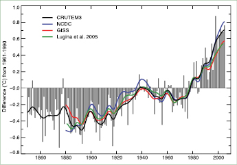
Figure 3.1. Annual anomalies of global land-surface air temperature (°C), 1850 to 2005, relative to the 1961 to 1990 mean for CRUTEM3 updated from Brohan et al. 2006 [JoC, MoS] ). The smooth curves show decadal variations (see Appendix 3.A ). The black curve from CRUTEM3 is compared with those from NCDC ( Smith and Reynolds, 2005 [JoC] ; blue), GISS ( Hansen et al., 2001 [JoC, ARC] ; red) and Lugina et al. 2005 [NPR] ; green).
Table 3.2. Linear trends in hemispheric and global land-surface air temperatures, SST (shown in table as HadSST2) and Nighttime Marine Air Temperature (NMAT; shown in table as HadMAT1). Annual averages, with estimates of uncertainties for CRU and HadSST2, were used to estimate trends. Trends with 5 to 95% confidence intervals and levels of significance(bold:<1%; italic,1–5%) were estimated by Restricted Maximum Likelihood (REML; see Appendix 3.A ), which allows for serial correlation (first order autoregression AR1) in the residuals of the data about the linear trend. The Durbin Watson D-statistic (not shown) for the residuals, after allowing for first-order serial correlation, never indicates significant positive serial correlation.
| Temperature Trend(oCper decade) | |||
|---|---|---|---|
| Dataset | 1850–2005 | 1901–2005 | 1979–2005 |
| Land: Northern Hemisphere | |||
| CRU (Brohan et al., 2006) | 0.063 ± 0.015 | 0.089 ± 0.025 | 0.328 ± 0.087 |
| NCDC (Smith and Reynolds, 2005) | 0.072 ± 0.026 | 0.344 ± 0.096 | |
| GISS (Hansen et al., 2001) | 0.083 ± 0.025 | 0.294 ± 0.074 | |
| Lugina et al. (2006) | 0.079 ± 0.029 | 0.301 ± 0.075 | |
| Land: Southern Hemisphere | |||
| CRU (Brohan et al., 2006) | 0.036 ± 0.024 | 0.077 ± 0.029 | 0.134 ± 0.070 |
| NCDC (Smith and Reynolds, 2005) | 0.057 ± 0.017 | 0.220 ± 0.093 | |
| GISS (Hansen et al., 2001) | 0.056 ± 0.012 | 0.085 ± 0.055 | |
| Lugina et al. (2005) | 0.058 ± 0.011 | 0.091 ± 0.048 | |
| Land: Globe | |||
| CRU (Brohan et al., 2006) | 0.054 ± 0.016 | 0.084 ± 0.021 | 0.268 ± 0.069 |
| NCDC (Smith and Reynolds, 2005) | 0.068 ± 0.024 | 0.315 ± 0.088 | |
| GISS (Hansen et al., 2001) | 0.069 ± 0.017 | 0.188 ± 0.069 | |
| Lugina et al. (2005) | 0.069 ± 0.020 | 0.203 ± 0.058 | |
| Ocean: Northern Hemisphere | |||
| UKMO HadSST2 (Rayner et al., 2006) | 0.042 ± 0.016 | 0.071 ± 0.029 | 0.190 ± 0.134 |
| UKMO HadMAT1 (Rayner et al., 2003) from 1861 | 0.038 ± 0.011 | 0.065 ± 0.020 | 0.186 ± 0.060 |
| Ocean: Southern Hemisphere | |||
| UKMO HadSST2 (Rayner et al., 2006) | 0.036 ± 0.013 | 0.068 ± 0.015 | 0.089 ± 0.041 |
| UKMO HadMAT1 (Rayner et al., 2003) from 1861 | 0.040 ± 0.012 | 0.069 ± 0.011 | 0.092 ± 0.050 |
| Ocean: Globe | |||
| UKMO HadSST2 (Rayner et al., 2006) | 0.038 ± 0.011 | 0.067 ± 0.015 | 0.133 ± 0.047 |
| UKMO HadMAT1 (Rayner et al., 2003) from 1861 | 0.039 ± 0.010 | 0.067 ± 0.013 | 0.135 ± 0.044 |
Further, small differences arise from the treatment of gaps in the data. The GISS gridding method favours isolated island and coastal sites, thereby reducing recent trends, and Lugina et al. 2005 [NPR] ) also obtain reduced recent trends owing to their optimal interpolation method that tends to adjust anomalies towards zero where there are few observations nearby (see, e.g., Hurrell and Trenberth, 1999 [PoC, JoC, MoS, SRC] ). The NCDC analysis, which begins in 1880, is higher than CRUTEM3 by between 0.1°C and 0.2°C in the first half of the 20th century and since the late 1990 s. This is probably because its anomalies have been interpolated to be spatially complete: an earlier but very similar version (CRUTEM2v; Jones and Moberg, 2003 [JoC, SRC] ) agreed very closely with NCDC when the global averages were calculated in the same way ( Vose et al., 2005b [JoC, SRC] ). Differences may also arise because the numbers of stations used by CRUTEM3, NCDC and GISS differ (4,349, 7,230 and >7,200 respectively), although many of the basic station data are in common. Differences in station numbers relate principally to CRUTEM3 requiring series to have sufficient data between 1961 and 1990 to allow the calculation of anomalies ( Brohan et al., 2006 [JoC, MoS] ). Further differences may have arisen from differing homogeneity adjustments (see also Appendix 3.B.2).
Trends and low-frequency variability of large-scale surface air temperature from the ERA-40 reanalysis and from CRUTEM2v ( Jones and Moberg, 2003 [JoC, SRC] ) are in general agreement from the late 1970 s onwards ( Simmons et al., 2004 [JoC, SRC] ). When ERA-40 is sub-sampled to match the Jones and Moberg coverage, correlations between monthly hemispheric- and continental-scale averages exceed 0.96, although trends in ERA-40 are then 0.03°C and 0.07°C per decade (NH and SH, respectively) lower than Jones and Moberg 2003 [JoC, SRC] ). The ERA-40 reanalysis is more homogeneous than previous reanalyses (see Section 3.2.1 and Appendix 3.B.5.4) but is not completely independent of the Jones and Moberg data ( Simmons et al., 2004 [JoC, SRC] ). The warming trends continue to be greatest over the continents of the NH (see maps in Section 3.2.2.7 ,Figures 3.9 and 3.10 ), in line with the TAR. Issues of homogeneity of terrestrial air temperatures are discussed in Appendix 3.B.2.
Table 3.2 provides trend estimates from a number of hemispheric and global temperature databases. Warming since 1979 in CRUTEM3 has been 0.27°C per decade for the globe, but 0.33°C and 0.13°C per decade for the NH and SH, respectively. Brohan et al. 2006 [JoC, MoS] and Rayner et al. 2006 [JoC] ) (see Section 3.2.2.3 )provide uncertainties for annual estimates, incorporating the effects of measurement and sampling error, and uncertainties regarding biases due to urbanisation and earlier methods of measuring SST. These factors are taken into account, although ignoring their serial correlation. In Table 3.2 ,the effects of persistence on error bars are accommodated using a red noise approximation, which effectively captures the main influences. For more extensive discussion see Appendix 3.A
From 1950 to 2004, the annual trends in minimum and maximum land-surface air temperature averaged over regions with data were 0.20°C per decade and 0.14°C per decade, respectively, with a trend in diurnal temperature range (DTR) of –0.07°C per decade ( Vose et al., 2005a [JoC, SRC] ; Figure 3.2 ). This is consistent with the TAR where data extended from 1950 to 1993; spatial coverage is now 71% of the terrestrial surface instead of 54% in the TAR, although tropical areas are still under-represented. Prior to 1950, insufficient data are available to develop global-scale maps of maximum and minimum temperature trends. For 1979 to 2004, the corresponding linear trends for the land areas where data are available were 0.29°C per decade for both maximum and minimum temperature with no trend for DTR. Diurnal temperature range is particularly sensitive to observing techniques, and monitoring it requires adherence to GCOS monitoring principles ( GCOS, 2004 [NPR] ). A map of the trend of annual DTR over the period 1979 to 2004 ( Section 3.2.2.7 , Figure 3.11 )is discussed later in the chapter.
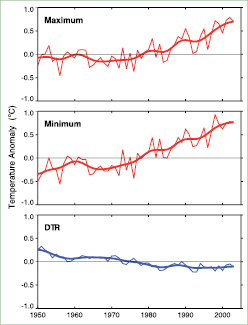
Figure 3.2. Annual anomalies of maximum and minimum temperatures and DTR (°C) relative to the 1961 to 1990 mean, averaged for the 71% of global land areas where data are available for 1950 to 2004 . The smooth curves show decadal variations (see Appendix 3.A ). Adapted from Vose et al. 2005a [JoC, SRC] ).
3.2.2.2 Urban Heat Islands and Land Use Effects
The modified land surface in cities affects the storage and radiative and turbulent transfers of heat and its partition into sensible and latent components (see Section 7.2 and Box 7.2 ). The relative warmth of a city compared with surrounding rural areas, known as the urban heat island (UHI) effect, arises from these changes and may also be affected by changes in water runoff, pollution and aerosols. Urban heat island effects are often very localised and depend on local climate factors such as windiness and cloudiness (which in turn depend on season), and on proximity to the sea. Section 3.3.2.4 discusses impacts of urbanisation on precipitation.
Many local studies have demonstrated that the microclimate within cities is on average warmer, with a smaller DTR, than if the city were not there. However, the key issue from a climate change standpoint is whether urban-affected temperature records have significantly biased large-scale temporal trends. Studies that have looked at hemispheric and global scales conclude that any urban-related trend is an order of magnitude smaller than decadal and longer time-scale trends evident in the series (e.g., Jones et al., 1990 [JoC, SRC] ; Peterson et al., 1999 [JoC, ARC] ). This result could partly be attributed to the omission from the gridded data set of a small number of sites (<1%) with clear urban-related warming trends. In a worldwide set of about 270 stations, Parker 2004 [JoC] , 2006 ) noted that warming trends in night minimum temperatures over the period 1950 to 2000 were not enhanced on calm nights, which would be the time most likely to be affected by urban warming. Thus, the global land warming trend discussed is very unlikely to be influenced significantly by increasing urbanisation ( Parker, 2006 [JoC] ). Over the conterminous USA, after adjustment for time-of-observation bias and other changes, rural station trends were almost indistinguishable from series including urban sites ( Peterson, 2003 [JoC, ARC] ; Figure 3.3 ,and similar considerations apply to China from 1951 to 2001 ( (Li et al., 2004 ) ). One possible reason for the patchiness of UHIs is the location of observing stations in parks where urban influences are reduced ( Peterson, 2003 [JoC, ARC] ). In summary, although some individual sites may be affected, including some small rural locations, the UHI effect is not pervasive, as all global-scale studies indicate it is a very small component of large-scale averages. Accordingly, this assessment adds the same level of urban warming uncertainty as in the TAR: 0.006°C per decade since 1900 for land, and 0.002°C per decade since 1900 for blended land with ocean, as ocean UHI is zero. These uncertainties are added to the cool side of the estimated temperatures and trends, as explained by Brohan et al. 2006 [JoC, MoS] ), so that the error bars in Section 3.2.2.4 ,Figures 3.6 and 3.7 and FAQ 3.1 ,Figure 1 are slightly asymmetric. The statistical significances of the trends in Table 3.2 and Section 3.2.2.4 , Table 3.3 take account of this asymmetry.
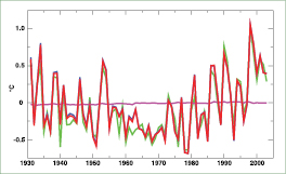
Figure 3.3. Anomaly (°C) time series relative to the 1961 to 1990 mean of the full US Historical Climatology Network (USHCN) data (red), the USHCN data without the 16% of the stations with populations of over 30,000 within 6 km in the year 2000 (blue), and the 16% of the stations with populations over 30,000 (green). The full USHCN set minus the set without the urban stations is shown in magenta. Both the full data set and the data set without the high-population stations had stations in all of the 2.5° latitude by 3.5° longitude grid boxes during the entire period plotted, but the subset of high-population stations only had data in 56% of these grid boxes. Adapted from Peterson and Owen 2005 [JoC, ARC] ).
( McKitrick and Michaels 2004 ) and de Laat and Maurellis 2006 [JoC] ) attempted to demonstrate that geographical patterns of warming trends over land are strongly correlated with geographical patterns of industrial and socioeconomic development, implying that urbanisation and related land surface changes have caused much of the observed warming. However, the locations of greatest socioeconomic development are also those that have been most warmed by atmospheric circulation changes (Sections 3.2.2.7 and 3.6.4 ), which exhibit large-scale coherence. Hence, the correlation of warming with industrial and socioeconomic development ceases to be statistically significant. In addition, observed warming has been, and transient greenhouse-induced warming is expected to be, greater over land than over the oceans( Chapter 10 ), owing to the smaller thermal capacity of the land.
Comparing surface temperature estimates from the NRA with raw station time series, Kalnay and Cai 2003 [JoC] ) concluded that more than half of the observed decrease in DTR in the eastern USA since 1950 was due to changes in land use, including urbanisation. This conclusion was based on the fact that the reanalysis did not explicitly include these factors, which would affect the observations. However, the reanalysis also did not explicitly include many other natural and anthropogenic effects, such as increasing greenhouse gases and observed changes in clouds or soil moisture ( Trenberth, 2004 [PoC, JoC, SRC] Vose et al. 2004 [JoC, SRC] ) showed that the adjusted station data for the region (for homogeneity issues, see Appendix 3.B.2) do not support Kalnay and Cai’s conclusions. Nor are Kalnay and Cai’s results reproduced in the ERA-40 reanalysis ( Simmons et al., 2004 [JoC, SRC] ). Instead, most of the changes appear related to abrupt changes in the type of data assimilated into the reanalysis, rather than to gradual changes arising from land use and urbanisation changes. Current reanalyses may be reliable for estimating trends since 1979 ( Simmons et al., 2004 [JoC, SRC] ) but are in general unsuited for estimating longer-term global trends, as discussed in Appendix 3.B.5.
Nevertheless, changes in land use can be important for DTR at the local-to-regional scale. For instance, land degradation in northern Mexico resulted in an increase in DTR relative to locations across the border in the USA ( Balling et al., 1998 [JoC] ), and agriculture affects temperatures in the USA ( Bonan, 2001 [JoC, ARC] ; Christy et al., 2006 [NotFound] ). Desiccation of the Aral Sea since 1960 raised DTR locally ( Small et al., 2001 [JoC] ). By processing maximum and minimum temperature data as a function of day of the week, Forster and Solomon 2003 [PoC, JoC, ARC] ) found a distinctive ‘weekend effect’ in DTR at stations examined in the USA, Japan, Mexico and China. The weekly cycle in DTR has a distinctive large-scale pattern with geographically varying sign, and strongly suggests an anthropogenic effect on climate, likely through changes in pollution and aerosols ( Jin et al., 2005 [JoC, SRC] ). Section 7.2 provides fuller discussion of the effects of land use changes.
3.2.2.3 Sea Surface Temperature and Marine Air Temperature
Most analyses of SST estimate the subsurface bulk temperature (i.e., the temperature in the uppermost few metres of the ocean), not the ocean skin temperature measured by satellites. For maximum resolution and data coverage, polar-orbiting infrared satellite data since 1981 can be used so long as the satellite ocean skin temperatures are adjusted to estimate bulk SST values through a calibration procedure (see e.g., Reynolds et al., 2002 [JoC] ; Rayner et al., 2003 [JoC] , 2006; Appendix 3.B.3). But satellite SST data alone have not been used as a major resource for estimating climate change because of their strong time-varying biases which are hard to completely remove, for example, as shown in Reynolds et al. 2002 [JoC] ) for the Pathfinder polar orbiting satellite SST data set ( Kilpatrick et al., 2001 [JoC] ). Figures 3.9 and 3.10 ( Section 3.2.2.7 )do, however, make use of spatial relationships based on adjusted satellite SST estimates after November 1981 to provide nearer-to-global coverage for the 1979 to 2005 period, ( and O’Carroll et al. 2006 ) ) have developed an analysis based on Along-Track Scanning Radiometers (ATSRs) with potential for the future. However, satellite data are unable to fill in estimates of surface temperature over or near sea ice areas.
Recent bulk SSTs estimated using ship and buoy data also have time-varying biases (e.g., Christy et al., 2001 [JoC, SRC] ; Kent and Kaplan, 2006 [MoS] ) that are larger than originally estimated by Folland et al. 1993 [PoC, JoC, SRC] ), but not large enough to prejudice conclusions about recent warming (see Appendix 3.B.3). As reported in the TAR, a combined physical-empirical method ( Folland and Parker, 1995 [PoC, JoC, SRC] ) is mainly used to estimate adjustments to ship SST data obtained up to 1941 to compensate for heat losses from uninsulated (mainly canvas) or partly insulated (mainly wooden) buckets. Details are given in Appendix 3.B.3.
The SST analyses of Rayner et al. 2003 [JoC] and Smith and Reynolds 2004 [JoC] ) are interpolated to fill missing data areas. The main problem for estimating climate variations in the presence of large data gaps is underestimation of change, as most interpolation procedures tend to bias the analysis towards the modern climatologies used in these data sets ( Hurrell and Trenberth, 1999 [PoC, JoC, MoS, SRC] ). To address non-stationary aspects, Rayner et al. 2003 [JoC] ) extracted the leading global covariance pattern, which represents long-term changes, before interpolating using reduced-space optimal interpolation (see Appendix 3.B.1); and Smith and Reynolds removed a smoothed, moving 15-year-average field before interpolating by a related technique.
Figure 3.4 ashows annual and decadally smoothed anomalies of global SST from the new, uninterpolated Hadley Centre SST data set version 2 (HadSST2) analysis ( Rayner et al., 2006 [JoC] ). Figure 3.4 aalso shows NMAT (referred to as HadMAT: Hadley Centre Marine Air Temperature data set), which is used to avoid daytime heating of ship decks ( Bottomley et al., 1990 [NPR] ). The global averages are ocean-area weighted sums (0.44 × NH + 0.56 × SH). The HadMAT analysis includes limited optimal interpolation ( Rayner et al., 2003 [JoC] ) and was chosen because of the demonstration by Folland et al. 2003 [PoC, JoC, SRC] ) of its skill in the sparsely observed South Pacific from the late 19th century onwards, but major gaps (e.g., the Southern Ocean) are not interpolated. Although HadMAT data have been corrected for warm biases during World War II they may still be too warm in the NH and too cool in the SH at that time( Figure 3.4 c,d). However, global HadSST2 and HadMAT generally agree well, especially after the 1880 s. The SST analysis in the TAR is included in Figure 3.4 a. The changes in SST since the TAR are generally fairly small, though the new SST analysis is warmer around 1880 and cooler in the 1950 s. The peak warmth in the early 1940 s is likely to have arisen partly from closely spaced multiple El Niño events ( Brönnimann et al., 2004 [NPR, JoC] ; see also Section 3.6.2 )and also due to the warm phase of the Atlantic Multi-decadal Oscillation (AMO; see Section 3.6.6 ). The HadMAT data generally confirm the hemispheric SST trends in the 20th century( Figure 3.4 c,d and Table 3.2 ). Overall, the SST data should be regarded as more reliable because averaging of fewer samples is needed for SST than for HadMAT to remove synoptic weather noise. However, the changes in SST relative to NMAT since 1991 in the tropical Pacific may be partly real ( Christy et al., 2001 [JoC, SRC] ). As the atmospheric circulation changes, the relationship between SST and surface air temperature anomalies can change along with surface fluxes. Interannual variations in the heat fluxes to the atmosphere can exceed 100 W m-2 locally in individual months, but the main prolonged variations occur with the El Niño-Southern Oscillation (ENSO), where changes in the central tropical Pacific exceed ±50 W m-2 for many months during major ENSO events ( Trenberth et al., 2002a [PoC, JoC, SRC] ).
Figure 3.4 bshows three time series of changes in global SST. Neither the HadSST2 series (as in Figure 3.4 a) nor the NCDC series include polar-orbiting satellite data because of possible time-varying biases that remain difficult to correct fully ( Rayner et al., 2003 [JoC] ). The Japanese series ( Ishii et al., 2005 [JoC, SRC] ; referred to as Centennial in-situ Observation-Based Estimates of SSTs (COBE-SST) from the Japan Meteorological Agency (JMA)) is also in situ except for the specification of sea ice. The warmest year globally in each SST record was 1998 (0.44°C, 0.38°C and 0.37°C above the 1961 to 1990 average for HadSST2, NCDC and COBE-SST, respectively). The five warmest years in all analyses have occurred after 1995 .
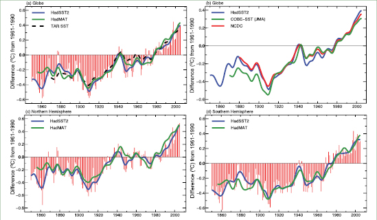
Figure 3.4. (a) Annual anomalies of global SST (HadSST2; red bars and blue solid curve), 1850 to 2005, and global NMAT (HadMAT, green curve), 1856 to 2005, relative to the 1961 to 1990 mean (°C) from the UK Meteorological Office (UKMO; Rayner et al., 2006 [JoC] ). The smooth curves show decadal variations (see Appendix 3.A ). The dashed black curve shows equivalent smoothed SST anomalies from the TAR. (b) Smoothed annual global SST anomalies, relative to 1961 to 1990 (°C), from HadSST2 (blue line, as in (a)), from NCDC ( Smith et al., 2005 [JoC] ; red line) and from COBE-SST ( Ishii et al., 2005 [JoC, SRC] ; green line). The latter two series begin later in the 19th century than HadSST2. (c,d) As in (a) but for the NH and SH showing only the UKMO series.
Understanding of the variability and trends in different oceans is still developing, but it is already apparent that they are quite different. The Pacific is dominated by ENSO and modulated by the Pacific Decadal Oscillation (PDO), which may provide ways of moving heat from the tropical ocean to higher latitudes and out of the ocean into the atmosphere ( Trenberth et al., 2002a [PoC, JoC, SRC] ), thereby greatly altering how trends are manifested. In the Atlantic, observations reveal the role of the AMO ( Folland et al., 1999 [NPR, PoC, SRC] ; Delworth and Mann, 2000 [PoC, JoC, MoS, ARC] ; Enfield et al., 2001 [JoC] ; Goldenberg et al., 2001 [JoC] ; Section 3.6.6 and Figure 3.33 ). The AMO is likely to be associated with the Thermohaline Circulation (THC), which transports heat northwards, thereby moderating the tropics and warming the high latitudes. In the Indian Ocean, interannual variability is small compared with the trend. Figure 3.5 presents latitude-time sections from 1900 for SSTs (from HadSST2) for the zonal mean across each ocean, filtered to remove fluctuations of less than about six years, including the ENSO signal. In the Pacific, the long-term warming is clearly evident, but punctuated by cooler episodes centred in the tropics, and no doubt linked to the PDO. The prolonged 1939 – 1942 El Niño shows up as a warm interval. In the Atlantic, the warming from the 1920 s to about 1940 in the NH was focussed on higher latitudes, with the SH remaining cool. This inter-hemispheric contrast is believed to be one signature of the THC ( Zhang and Delworth, 2005 [JoC, MoS, ARC] ). The subsequent relative cooling in the NH extratropics and the more recent intense warming in NH mid-latitudes was predominantly a multi-decadal variation of SST; only in the last decade is an overall warming signal clearly emerging. Therefore, the recent strong warming appears to be related in part to the AMO in addition to a global warming signal( Section 3.6.6 ). The cooling in the northwestern North Atlantic just south of Greenland, reported in the SAR, has now been replaced by strong warming (see also Section 3.2.2.7 ,Figures 3.9 and 3.10 ;also Figures 5.1 and 5.2 for ocean heat content). The Indian Ocean also reveals a poorly observed warm interval in the early 1940 s, and further shows the fairly steady warming in recent years. The multi-decadal variability in the Atlantic has a much longer time scale than that in the Pacific, but it is noteworthy that all oceans exhibit a warm period around the early 1940 s.
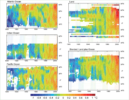
Figure 3.5. Latitude-time sections of zonal mean temperature anomalies (°C) from 1900 to 2005, relative to the 1961 to 1990 mean. Left panels: SST annual anomalies across each ocean from HadSST2 ( Rayner et al., 2006 [JoC] ). Right panels: Surface temperature annual anomalies for land (top, CRUTEM3) and land plus ocean (bottom, HadCRUT3). Values are smoothed with the 5-point filter to remove fluctuations of less than about six years (see Appendix 3.A ); and white areas indicate missing data.
3.2.2.4 Land and Sea Combined Temperature: Global, Northern Hemisphere, Southern Hemisphere and Zonal Means
Gridded data sets combining land-surface air temperature and SST anomalies have been developed and maintained by three groups: CRU with the UKMO Hadley Centre in the UK (HadCRUT3; Brohan et al., 2006 [JoC, MoS] ) and NCDC ( Smith and Reynolds, 2005 [JoC] ) and GISS ( Hansen et al., 2001 [JoC, ARC] ) in the USA. Although the component data sets differ slightly (see Sections 3.2.2.1 and 3.2.2.3 )and the combination methods also differ, trends are similar. Table 3.3 provides comparative estimates of linear trends. Overall warming since 1901 has been a little less in the NCDC and GISS analysis than in the HadCRUT3 analysis. All series indicate that the warmest five years have occurred after 1997, although there is slight disagreement about the ordering. The HadCRUT3 data set shows 1998 as warmest, while 2005 is warmest in NCDC and GISS data. Thus the year 2005, with no El Niño, was about as warm globally as 1998 with its major El Niño effects. The GISS analysis of 2005 interpolated the exceptionally warm conditions in the extreme north of Eurasia and North America over the Arctic Ocean (see Figure 3.5 ). If the GISS data for 2005 are averaged only south of 75°N, then 2005 is cooler than 1998 . In addition, there were relatively cool anomalies in 2005 in HadCRUT3 in parts of Antarctica and the Southern Ocean, where sea ice coverage (see Chapter4 )has not declined.
Table 3.3. Linear trends (°C per decade) in hemispheric and global combined land-surface air temperatures and SST. Annual averages, along with estimates of uncertainties for CRU/UKMO (HadCRUT3), were used to estimate trends. For CRU/UKMO, global annual averages are the simple average of the two hemispheres. For NCDC and GISS the hemispheres are weighted as in Section 3.2.2.1 .Trends are estimated and presented as in Table 3.2. R2 is the squared trend correlation (%). The Durbin Watson D-statistic (not shown) for the residuals, after allowing for first-order serial correlation, never indicated significant positive serial correlation, and plots of the residuals showed virtually no long-range persistence.
| Temperature Trend(oCper decade) | |||
|---|---|---|---|
| Dataset | 1850–2005 | 1901–2005 | 1979–2005 |
| Northern Hemisphere | |||
| CRU/UKMO (Brohan et al., 2006) |
0.047 ± 0.013 R2=54 |
0.075 ± 0.023 R2=63 |
0.234 ± 0.070 R2=69 |
| NCDC (Smith and Reynolds, 2005) |
|
0.063 ± 0.022 R2=55 |
0.245 ± 0.062 R2=72 |
| Southern Hemisphere |
|
|
|
| CRU/UKMO (Brohan et al., 2006) |
0.038 ± 0.014 R2=51 |
0.068 ± 0.017 R2=74 |
0.092 ± 0.038 R2=48 |
| NCDC (Smith and Reynolds, 2005) |
|
0.066 ± 0.009 R2=82 |
0.096 ± 0.038 R2=58 |
| Globe |
|
|
|
| CRU/UKMO (Brohan et al., 2006) |
0.042 ± 0.012 R2=57 |
0.071 ± 0.017 R2=74 |
0.163 ± 0.046 R2=67 |
| NCDC (Smith and Reynolds, 2005) | 0.064 ± 0.016R2=71 | 0.174 ± 0.051R2=72 | |
| GISS (Hansen et al., 2001) | 0.060 ± 0.014R2=70 | 0.170 ± 0.047R2=67 | |
Hemispheric and global series based on Brohan et al. 2006 [JoC, MoS] ) are shown in Figure 3.6 and tropical and polar series in Figure 3.7 .Owing to the sparsity of SST data, the polar series are for land only. The recent warming is strongest in the NH extratropics, while El Niño events are clearly evident in the tropics, particularly the 1997 – 1998 event that makes 1998 the warmest year in HadCRUT3. The warming over land in the Arctic north of 65°N( Figure 3.7 )is more than double the warming in the global mean from the 19th century to the 21st century and also from about the late 1960 s to the present. In the arctic series, 2005 is the warmest year. A slightly longer warm period, almost as warm as the present, was observed from the late 1920 s to the early 1950 s. Although data coverage was limited in the first half of the 20th century, the spatial pattern of the earlier warm period appears to have been different from that of the current warmth. In particular, the current warmth is partly linked to the Northern Annular Mode (NAM; see Section 3.6.4 )and affects a broader region ( Polyakov et al., 2003 [JoC] ). Temperatures over mainland Antarctica (south of 65°S) have not warmed in recent decades ( Turner et al., 2005 [JoC] ), but it is virtually certain that there has been strong warming over the last 50 years in the Antarctic Peninsula region ( Turner et al., 2005 [JoC] ; see the discussion of changes in the Southern Annular Mode (SAM) and Figure 3.32 in Section 3.6.5 ).
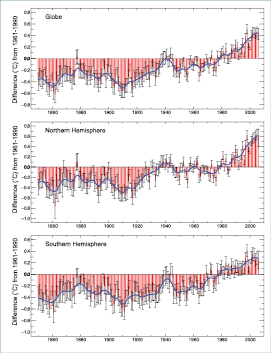
Figure 3.6. Global and hemispheric annual combined land-surface air temperature and SST anomalies (°C) (red) for 1850 to 2006 relative to the 1961 to 1990 mean, along with 5 to 95% error bar ranges, from HadCRUT3 (adapted from Brohan et al., 2006 [JoC, MoS] ). The smooth blue curves show decadal variations (see Appendix 3.A ).
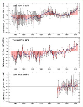
Figure 3.7. Annual temperature anomalies (°C) up to 2005, relative to the 1961 to 1990 mean (red) with 5 to 95% error bars. The tropical series (middle) is combined land-surface air temperature and SST from HADCRUT3 (adapted from Brohan et al., 2006 [JoC, MoS] ). The polar series (top and bottom) are land-only from CRUTEM3, because SST data are sparse and unreliable in sea ice zones. The smooth blue curves show decadal variations (see Appendix 3.A ).
3.2.2.5 Consistency between Land and Ocean Surface Temperature Changes
The course of temperature change over the 20th century, revealed by the independent analysis of land air temperatures, SST and NMAT, is generally consistent( Figure 3.8 ). Warming occurred in two distinct phases ( 1915 – 1945 and since 1975 ), and it has been substantially stronger over land than over the oceans in the later phase, as shown also by the trends in Table 3.2 .The land component has also been more variable from year to year (compare Figures 3.1 and 3.4 a,c,d). Much of the recent difference between global SST (and NMAT) and global land air temperature trends has arisen from accentuated warming over the continents in the mid-latitude NH( Section 3.2.2.7 ,Figures 3.9 and 3.10 ). This is likely to be related to greater evaporation and heat storage in the ocean, and in particular to atmospheric circulation changes in the winter half-year due to the North Atlantic Oscillation (NAO)/NAM (see discussion in Section 3.6.4 ). Accordingly the differences between NH and SH temperatures follow a course similar to the plot of land air temperature minus SST shown in Figure 3.8 .
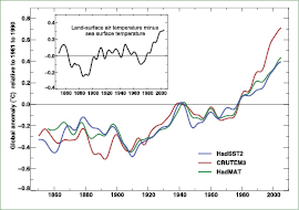
Figure 3.8. Annual anomalies (°C) of global average SST (blue curve, begins 1850 ), NMAT (green curve, begins 1856 ) and land-surface air temperature (red curve, begins 1850 ) to 2005, relative to their 1961 to 1990 means ( Brohan et al., 2006 [JoC, MoS] ; Rayner et al., 2006 [JoC] ). The smooth curves show decadal variations (see Appendix 3.A ). Inset shows the smoothed differences between the land-surface air temperature and SST anomalies (i.e., red minus blue).
3.2.2.6 Temporal Variability of Global Temperatures and Recent Warming
The standard deviation of the HadCRUT3 annual average temperatures for the globe for 1850 to 2005 shown in Figure 3.6 is 0.24°C. The greatest difference between two consecutive years in the global average since 1901 is 0.29°C between 1976 and 1977, demonstrating the importance of the 0.75°C and 0.74°C temperature increases (the HadCRUT3 linear trend estimates for 1901 to 2005 and 1906 to 2005, respectively) in a centennial time-scale context. However, both trends are small compared with interannual variations at one location, and much smaller than day-to-day variations( Table 3.1 ).
The principal conclusion from the three global analyses is that the global average surface temperature trend has very likely been slightly more than 0.65°C ± 0.2°C over the period from 1901 to 2005 ( Table 3.3 ), a warming greater than any since at least the 11th century (see Chapter6 ). A HadCRUT3 linear trend over the 1906 to 2005 period yields a warming of 0.74°C ± 0.18°C, but this rate almost doubles for the last 50 years (0.64°C ± 0.13°C for 1956 to 2005; see FAQ 3.1 ). Clearly, the changes are not linear and can also be characterised as level prior to about 1915, a warming to about 1945, levelling out or even a slight decrease until the 1970 s, and a fairly linear upward trend since then( Figure 3.6 and FAQ 3.1 ). Considered this way, the overall warming from the average of the first 50-year period ( 1850 – 1899 ) through 2001 to 2005 is 0.76°C ± 0.19°C. Clearly, the world’s surface temperature has continued to increase since the TAR and the trend when computed in the same way as in the TAR remains 0.6°C over the 20th century. In view of Section 3.2.2.2 and the dominance of the globe by ocean, the influence of urbanisation on these estimates is estimated to be very small. The last 12 complete years ( 1995 – 2006 ) now contain 11 of the 12 warmest years since 1850, the earliest year for which comparable records are available. Only 1996 is not in this list – replaced by 1990 . 2002 to 2005 are the 3rd, 4th, 5th and 2nd warmest years in the series, with 1998 the warmest in HadCRUT3 but with 2005 and 1998 switching order in GISS and NCDC. The HadCRUT3 surface warming trend over 1979 to 2005 was more than 0.16°C per decade, that is, a total warming of 0.44°C ± 0.12°C (the error bars overlap those of NCDC and GISS). During 2001 to 2005, the global average temperature anomaly has been 0.44°C above the 1961 – 1990 average. The value for 2006 is close to the 2001 to 2005 average.
3.2.2.7 Spatial Trend Patterns
Figure 3.9 illustrates the spatial patterns of annual surface temperature changes for 1901 to 2005 and 1979 to 2005, and Figure 3.10 shows seasonal trends for 1979 to 2005 . All maps clearly indicate that differences in trends between locations can be large, particularly for shorter time periods. For the century-long period, warming is statistically significant over most of the world’s surface with the exception of an area south of Greenland and three smaller regions over the southeastern USA and parts of Bolivia and the Congo basin. The lack of significant warming at about 20% of the locations ( Karoly and Wu, 2005 [JoC, ARC] ), and the enhanced warming in other places, is likely to be a result of changes in atmospheric circulation (see Section 3.6 ). Warming is strongest over the continental interiors of Asia and northwestern North America and over some mid-latitude ocean regions of the SH as well as southeastern Brazil. In the recent period, some regions have warmed substantially while a few have cooled slightly on an annual basis( Figure 3.9 ). Southwest China has cooled since the mid-20th century ( (Ren et al., 2005 ) ), but most of the cooling locations since 1979 have been oceanic and in the SH, possibly through changes in atmospheric and oceanic circulation related to the PDO and SAM (see discussion in Section 3.6.5 ). Warming dominates most of the seasonal maps for the period 1979 onwards, but weak cooling has affected a few regions, especially the mid-latitudes of the SH oceans, but also over eastern Canada in spring, possibly in relation to the strengthening NAO (see Section 3.6.4 , Figure 3.30 ). Warming in this period was strongest over western North America, northern Europe and China in winter, Europe and northern and eastern Asia in spring, Europe and North Africa in summer and northern North America, Greenland and eastern Asia in autumn( Figure 3.10 ).
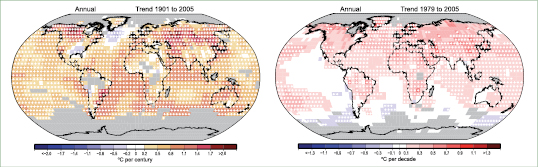
Figure 3.9. Linear trend of annual temperatures for 1901 to 2005 (left; °C per century) and 1979 to 2005 (right; °C per decade). Areas in grey have insufficient data to produce reliable trends. The minimum number of years needed to calculate a trend value is 66 years for 1901 to 2005 and 18 years for 1979 to 2005 . An annual value is available if there are 10 valid monthly temperature anomaly values. The data set used was produced by NCDC from Smith and Reynolds 2005 [JoC] ). Trends significant at the 5% level are indicated by white + marks.
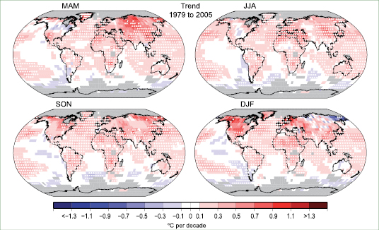
Figure 3.10. Linear trend of seasonal MAM, JJA, SON and DJF temperature for 1979 to 2005 (°C per decade). Areas in grey have insufficient data to produce reliable trends. The minimum number of years required to calculate a trend value is 18. A seasonal value is available if there are two valid monthly temperature anomaly values. The dataset used was produced by NCDC from Smith and Reynolds 2005 [JoC] ). Trends significant at the 5% level are indicated by white + marks.
No single location follows the global average, and the only way to monitor the globe with any confidence is to include observations from as many diverse places as possible. The importance of regions without adequate records is determined from complete model reanalysis fields ( Simmons et al., 2004 [JoC, SRC] ). The importance of the missing areas for hemispheric and global averages is incorporated into the errors bars in Figure 3.6 (see Brohan et al., 2006 [JoC, MoS] ). Error bars are generally larger in the more data-sparse SH than in the NH; they are larger before the 1950 s and largest of all in the 19th century.
Figure 3.11 shows annual trends in DTR from 1979 to 2004 . The decline in DTR since 1950 reported in the TAR has now ceased, as confirmed by Figure 3.2 .Since 1979, daily minimum temperature increased in most areas except western Australia and southern Argentina, and parts of the western Pacific Ocean; and daily maximum temperature also increased in most regions except northern Peru, northern Argentina, northwestern Australia, and parts of the North Pacific Ocean ( Vose et al., 2005a [JoC, SRC] ). The changes reported here appear inconsistent with Dai et al. 2006 [Ambiguous] ) who reported decreasing DTR in the USA, but this arises partly because Dai et al. 2006 [Ambiguous] ) included the high DTR years 1976 to 1978 . Furthermore, Figure 3.11 is supported by many other recent regional-scale analyses.
Changes in cloud cover and precipitation explained up to 80% of the variance in historical DTR series for the USA, Australia, mid-latitude Canada and the former Soviet Union during the 20th century ( Dai et al., 1999 [PoC, JoC, SRC] ). Cloud cover accounted for nearly half of the change in the DTR in Fennoscandia during the 20th century ( Tuomenvirta et al., 2000 [JoC] ). Variations in atmospheric circulation also affect DTR. Changes in the frequency of certain synoptic weather types resulted in a decline in DTR during the cold half-year in the Arctic ( Przybylak, 2000 [JoC] ). A positive phase of the NAM (see Section 3.6.4 )is associated with increased DTR in the northeastern USA and Canada ( Wettstein and Mearns, 2002 [JoC, ARC] ). Variations in sea level pressure patterns and associated changes in cloud cover partially accounted for increasing trends in cold-season DTR in the northwestern USA and decreasing trends in the south-central USA ( Durre and Wallace, 2001 [JoC] ). The relationship between DTR and anthropogenic forcings is complex, as these forcings can affect atmospheric circulation, as well as clouds through both greenhouses gases and aerosols.
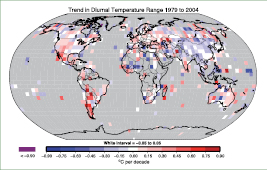
Figure 3.11. Linear trend in annual mean DTR for 1979 to 2004 (°C per decade). Grey regions indicate incomplete or missing data (after Vose et al., 2005a [JoC, SRC] ).
3.3 Changes in Surface Climate: Precipitation, Drought and Surface Hydrology
3.3.1 Background
Temperature changes are one of the more obvious and easily measured changes in climate, but atmospheric moisture, precipitation and atmospheric circulation also change, as the whole system is affected. Radiative forcing alters heating, and at the Earth’s surface this directly affects evaporation as well as sensible heating (see Box 7.1 ). Further, increases in temperature lead to increases in the moisture-holding capacity of the atmosphere at a rate of about 7% per °C( Section 3.4.2 ). Together these effects alter the hydrological cycle, especially characteristics of precipitation (amount, frequency, intensity, duration, type) and extremes ( Trenberth et al., 2003 [PoC, JoC, SRC] ). In weather systems, convergence of increased water vapour leads to more intense precipitation, but reductions in duration and/or frequency, given that total amounts do not change much. The extremes are addressed in Section 3.8.2.2 .Expectations for changes in overall precipitation amounts are complicated by aerosols. Because aerosols block the Sun, surface heating is reduced. Absorption of radiation by some, notably carbonaceous, aerosols directly heats the aerosol layer that may otherwise have been heated by latent heat release following surface evaporation, thereby reducing the strength of the hydrological cycle. As aerosol influences tend to be regional, the net expected effect on precipitation over land is especially unclear. This section discusses most aspects of the surface hydrological cycle, except that surface water vapour is included with other changes in atmospheric water vapour in Section 3.4.2 .
Difficulties in the measurement of precipitation remain an area of concern in quantifying the extent to which global- and regional-scale precipitation has changed (see Appendix 3.B.4). In situ measurements are especially affected by wind effects on the gauge catch, particularly for snow but also for light rain. For remotely sensed measurements (radar and space-based), the greatest problems are that only measurements of instantaneous rate can be made, together with uncertainties in algorithms for converting radiometric measurements (radar, microwave, infrared) into precipitation rates at the surface. Because of measurement problems, and because most historical in situ-based precipitation measurements are taken on land leaving the majority of the global surface area under-sampled, it is useful to examine the consistency of changes in a variety of complementary moisture variables. These include both remotely-sensed and gauge-measured precipitation, drought, evaporation, atmospheric moisture, soil moisture and stream flow, although uncertainties exist with all of these variables as well ( (Huntington, 2006 ) ).
3.3.2 Changes in Large-scale Precipitation
3.3.2.1 Global Land Areas
Trends in global annual land precipitation were analysed using data from the GHCN, using anomalies with respect to the 1981 to 2000 base period ( Vose et al., 1992 [NPR, SRC] ; Peterson and Vose, 1997 [JoC, SRC] ). The observed GHCN linear trend( Figure 3.12 )over the 106-year period from 1900 to 2005 is statistically insignificant, as is the CRU linear trend up to 2002 ( Table 3.4 b). However, the global mean land changes( Figure 3.12 )are not at all linear, with an overall increase until the 1950 s, a decline until the early 1990 s and then a recovery. Although the global land mean is an indicator of a crucial part of the global hydrological cycle, it is difficult to interpret as it is often made up of large regional anomalies of opposite sign.
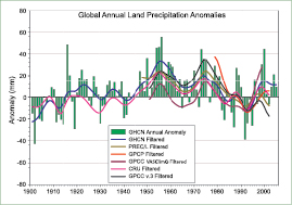
Figure 3.12. Time series for 1900 to 2005 of annual global land precipitation anomalies (mm) from GHCN with respect to the 1981 to 2000 base period. The smooth curves show decadal variations (see Appendix 3.A )for the GHCN ( Peterson and Vose, 1997 [JoC, SRC] ), PREC/L ( Chen et al., 2002 [JoC] ), GPCP ( Adler et al., 2003 [JoC, SRC] ), GPCC ( Rudolf et al., 1994 [NPR] ) and CRU ( Mitchell and Jones, 2005 [SRC] ) data sets.
There are several other global land precipitation data sets covering more recent periods: Table 3.4 agives their characteristics, and the linear trends and their significance are given in Table 3.4 b. There are a number of differences in processing, data sources and time periods that lead to the differences in the trend estimates. All but one data set (GHCN) are spatially infilled by either interpolation or the use of satellite estimates of precipitation. The Precipitation Reconstruction over Land (PREC/L) data ( Chen et al., 2002 [JoC] ) include GHCN data, synoptic data from the National Oceanic and Atmospheric Administration (NOAA) Climate Prediction Center’s Climate Anomaly Monitoring System (CAMS), and the Global Precipitation Climatology Project (GPCP) data ( Adler et al., 2003 [JoC, SRC] ), and are a blend of satellite and gauge data. The Global Precipitation Climatology Centre (GPCC; updated from Rudolf et al., 1994 [NPR] ) provides monthly data from surface gauges on several grids constructed using GPCC sources (including data from CRU, GHCN, a Food and Agriculture Organization (FAO) database and many nationally provided data sets). The data set designated GPCC VASClimO ( Beck et al., 2005 [NPR, SRC] ) uses only those quasi-continuous stations whose long-term homogeneity can be assured, while GPCC v.3 has used all available stations to provide more complete spatial coverage. Gridding schemes also vary and include optimal interpolation and grid-box averaging of areally weighted station anomalies. The CRU data set is from Mitchell and Jones 2005 [SRC] ).
Table 3.4. (a) Characteristics and references of the six global land-area precipitation data sets used to calculate trends. (b) Global land precipitation trends (mm per decade). Trends with 5 and 95% confidence intervals and levels of significance (italic, 1–5%) were estimated by REML (see Appendix 3.A ), which allows for serial correlation in the residuals of the data about the linear trend. All trends are based on annual averages without estimates of intrinsic uncertainties. (a)
| Series | Period of Record | Gauge only | Satellite and gauge | Spatial infilling | Reference |
|---|---|---|---|---|---|
| GHCN | 1900–2005 | X | No | Vose et al., 1992 | |
| PREC/L | 1948–2002 | X | Yes | Chen et al., 2002 | |
| GPCP | 1979–2002 | X | Yes | Adler et al., 2003 | |
| GPCC VASClimO | 1951–2000 | X | Yes | Beck et al., 2005 | |
| GPCC v.3 | 1951–2002 | X | Yes | Rudolf et al., 1994 | |
| CRU | 1901–2002 | X | Yes | Mitchell and Jones, 2005 |
| Precipitation Trend (mm per decade) | |||
|---|---|---|---|
| Series | 1901–2005 | 1951–2005 | 1979–2005 |
| PREC/L | –5.10 ± 3.25a | –6.38 ± 8.78a | |
| CRU | 1.10 ± 1.50a | –3.87 ± 3.89a | –0.90 ± 16.24a |
| GHCN | 1.08 ± 1.87 | –4.56 ± 4.34 | 4.16 ± 12.44 |
| GPCC VASClimO | 1.82 ± 5.32b | 12.82 ± 21.45b | |
| GPCC v.3 | –6.63 ± 5.18a | –14.64 ± 11.67a | |
| GPCP | –15.60 ± 19.84a | ||
For 1951 to 2005, trends range from –7 to +2 mm per decade and 5 to 95% error bars range from 3.2 to 5.3 mm per decade. Only the updated PREC/L series ( Chen et al., 2002 [JoC] ) trend and the GPCC v.3 trend appear to be statistically significant, but the uncertainties, as seen in the different estimates, undermine that result. For 1979 to 2005, GPCP data are added and trends range from –16 to +13 mm per decade but none is significant. Nevertheless, the discrepancies in trends are substantial, and highlight the difficulty of monitoring a variable such as precipitation that has large variability in both space and time. On the other hand, Figure 3.12 also suggests that interannual fluctuations have some overall reproducibility for land as a whole. The lag-1 autocorrelation of the residuals from the fitted trend (i.e., the de-trended persistence) is in the range 0.3 to 0.5 for the PREC/L, CRU and GHCN series but 0.5 to 0.7 for the two GPCC and the GPCP series. This suggests that either the limited sampling by in situ gauge data adds noise, or systematic biases lasting a few years (the lifetime of a satellite) are afflicting the GPCP data, or a combination of the two.
3.3.2.2 Spatial Patterns of Precipitation Trends
The spatial patterns of trends in annual precipitation (% per century or per decade) during the periods 1901 to 2005 and 1979 to 2005 are shown in Figure 3.13 .The observed trends over land areas were calculated using GHCN station data interpolated to a 5° × 5° latitude/longitude grid. For most of North America, and especially over high-latitude regions in Canada, annual precipitation has increased during the 105-year period. The primary exception is over the southwest USA, northwest Mexico and the Baja Peninsula, where the trend in annual precipitation has been negative (1 to 2% per decade) as drought has prevailed in recent years. Across South America, increasingly wet conditions were observed over the Amazon Basin and southeastern South America, including Patagonia, while negative trends in annual precipitation were observed over Chile and parts of the western coast of the continent. The largest negative trends in annual precipitation were observed over western Africa and the Sahel. After having concluded that the effect of changing rainfall-gauge networks on Sahel rainfall time series is small, Dai et al. 2004b [JoC, SRC] ) noted that Sahel rainfall in the 1990 s has recovered considerably from the severe dry years in the early 1980 s (see Section 3.7.4 and Figure 3.37 ). A drying trend is also evident over southern Africa since 1901 . Over much of northwestern India the 1901 to 2005 period shows increases of more than 20% per century, but the same area shows a strong decrease in annual precipitation for the 1979 to 2005 period. Northwestern Australia shows areas with moderate to strong increases in annual precipitation over both periods. Over most of Eurasia, increases in precipitation outnumber decreases for both periods.
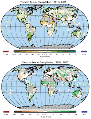
Figure 3.13. Trend of annual land precipitation amounts for 1901 to 2005 (top, % per century) and 1979 to 2005 (bottom, % per decade), using the GHCN precipitation data set from NCDC. The percentage is based on the means for the 1961 to 1990 period. Areas in grey have insufficient data to produce reliable trends. The minimum number of years required to calculate a trend value is 66 for 1901 to 2005 and 18 for 1979 to 2005 . An annual value is complete for a given year if all 12 monthly percentage anomaly values are present. Note the different colour bars and units in each plot. Trends significant at the 5% level are indicated by black + marks.
To assess the expected large regional variations in precipitation trends, Figure 3.14 presents time series of annual precipitation. The regions are 19 of those defined in Table 11.1 (see Section 11.1) and illustrated in Figure 11.26. The GHCN precipitation data set from NCDC was used, and the CRU decadal values allow the reproducibility to be assessed. Based on this, plots for four additional regions (Greenland, Sahara, Antarctica and the Tibetan Plateau) were not included, as precipitation data for these were not considered sufficiently reliable, nor was the first part of the Alaskan series (prior to 1935 ). Some discrepancies between the decadal variations are still evident at times, mostly owing to different subsets of stations and some stations coming in or dropping out, but overall the confidence in what is presented is quite high. Figure 3.15 presents a latitude-time series of zonal averages over land.
In the tropics, precipitation is highly seasonal, consisting of a dry season and a wet season in association with the summer monsoon. These aspects are discussed in more detail in Section 3.7 .Downward trends are strongest in the Sahel (see Section 3.7.4 )but occur in both western and eastern Africa in the past 50 years, and are reflected in the zonal means. The downward trends in this zone are also found in southern Asia. The linear trends of rainfall decreases for 1900 to 2005 were 7.5% in both the western Africa and southern Asia regions (significant at <1%). The area of the latter region is much greater than India, whose rainfall features strong variability but little in the way of a century-scale trend. Southern Africa also features a strong overall downward trend, although with strong multi-decadal variability present. Often the change in rainfall in these regions occurs fairly abruptly, and in several cases occurs around the same time in association with the 1976 – 1977 climate shift ( Wang and Ding, 2006 [JoC, SRC] ). The timing is not the same everywhere, however, and the downward shift occurred earlier in the Sahel (see also Section 3.7.4 , Figure 3.37 ). The main location with different trends at low latitudes is over Australia, but it is clear that large interannual variability, mostly ENSO-related, is dominant (note also the expanded vertical scales for Australia). The apparent upward trend occurs due to two rather wet spells in northern Australia in the early 1970 s and 1990 s, when it was dry in Southeast Asia (see also Section 3.7.2 ). Also of note in Australia is the marked downward trend in the far southwest characterised by a downward shift around 1975 ( Figure 3.13 ).
Figure 3.14. Precipitation for 1900 to 2005 . The central map shows the annual mean trends (% per century). Areas in grey have insufficient data to produce reliable trends. The surrounding time series of annual precipitation displayed (% of mean, with the mean given at top for 1961 to 1990 ) are for the named regions as indicated by the red arrows. The GHCN precipitation from NCDC was used for the annual green bars and black for decadal variations (see Appendix 3.A ), and for comparison the CRU decadal variations are in magenta. The range is +30 to –30% except for the two Australian panels. The regions are a subset of those defined in Table 11.1 (Section 11.1) and include: Central North America, Western North America, Alaska, Central America, Eastern North America, Mediterranean, Northern Europe, North Asia, East Asia, Central Asia, Southeast Asia, Southern Asia, Northern Australia, Southern Australia, Eastern Africa, Western Africa, Southern Africa, Southern South America, and the Amazon.
At higher latitudes, especially from 30°N to 85°N, quite distinct upward trends are evident in many regions and these are reflected in the zonal means( Figure 3.15 ). Central North America, eastern North America, northern Europe, northern Asia and central Asia (east of the Caspian Sea) all experienced upward linear trends of between 6 and 8% from 1900 to 2005 (all significant at <5%). These regions all experience snowfall (see also Section 3.3.2.3 )and part of the upward trend may arise from changes in efficiency of catching snow, especially in northern Asia. However, there is ample evidence that these trends are real (see Section 3.3.4 ), and they extend from North America to Europe across the North Atlantic as evidenced by ocean freshening, documented in Sections 5.2.3 and 5.3.2 .Western North America shows longer time-scale variability, principally due to the severe drought in the 1930 s and lesser events more recently. Note the tendency for inverse variations between northern Europe and the Mediterranean, associated with changes in the NAO (see Section 3.6.4 ). Southern Europe and parts of central Europe, as well as North Africa, are characterised by a drier winter (DJF) during the positive phase of the NAO, while the reverse is true in the British Isles, Fennoscandia and northwestern Russia.
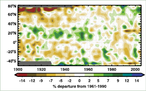
Figure 3.15. Latitude-time section of zonal average annual anomalies for precipitation (%) over land from 1900 to 2005, relative to their 1961 to 1990 means. Values are smoothed with the 5-point filter to remove fluctuations of less than about six years (see Appendix 3.A ). The colour scale is nonlinear and grey areas indicate missing data.
In the SH, Amazonia and southern South America feature opposite changes, as the South American monsoon features shifted southwards (see Section 3.7.3 ). This movement was in association with changes in ENSO and the 1976 – 1977 climate shift. The result is a pronounced upward trend in Argentina and the La Plata River Basin, but not in Chile (where the main declines in precipitation are evident in the austral summer (DJF) and autumn (MAM; Figure 3.13 ). Decadal-scale variations over Amazonia are also out of phase with the Central American region to the north, which in turn has out-of-phase variations with western North America, again suggestive of latitudinal changes in monsoon features. East and Southeast Asia show hardly any long-term changes, with both having plentiful rains in the 1950 s. At interannual time scales there are a number of surprisingly strong correlations: Amazonia is correlated with northern Australia (0.44, significant at <1%) and also Southeast Asia (0.55, <1%), while southern South America is inversely correlated with western Africa (−0.51, <1%). The correlations are surprising because they are based on high-frequency relationships and barely change when the smoothed series are used.
3.3.2.3 Changes in Snowfall
Winter precipitation has increased at high latitudes, although uncertainties exist because of changes in undercatch, especially as snow changes to rain. Snow cover changes are discussed in Section 4.2 .Annual precipitation for the circumpolar region north of 50°N has increased during the past 50 years (not shown) by approximately 4% but this increase has not been homogeneous in time and space ( Groisman et al., 2003 [NPR, SRC] , 2005 ). Statistically significant increases were documented over Fennoscandia, coastal regions of northern North America ( Groisman et al., 2005 [SRC] ), most of Canada (particularly northern regions) up until at least 1995 when the analysis ended ( Stone et al., 2000 [ARC] ), the permafrost-free zone of Russia ( Groisman and Rankova, 2001 [JoC, SRC] ) and the entire Great Russian Plain ( Groisman et al., 2005 [SRC] , 2007 ). However, there were no discernible changes in summer and annual precipitation totals over northern Eurasia east of the Ural Mountains ( Gruza et al., 1999 [JoC] ; Sun and Groisman, 2000 [JoC, SRC] ; Groisman et al., 2005 [SRC] , 2007 ). Rainfall (liquid precipitation) has increased during the past 50 years over western portions of North America and Eurasia north of 50°N by about 6%. Rising temperatures have generally resulted in rain rather than snow in locations and seasons where climatological average ( 1961 – 1990 ) temperatures were close to 0°C. The liquid precipitation season has become longer by up to three weeks in some regions of the boreal high latitudes over the last 50 years ( Cayan et al., 2001 [JoC, SRC] ; Groisman et al., 2001 [Ambiguous] ; Easterling, 2002 [JoC, ARC] ; Groisman et al., 2005 [SRC] , 2007 ) owing, in particular, to an earlier onset of spring. Therefore, in some regions (southern Canada and western Russia), snow has provided a declining fraction of total annual precipitation ( Groisman et al., 2003 [NPR, SRC] , 2005, 2007 ). In other regions, particularly north of 55°N, the fraction of annual precipitation falling as snow in winter has changed little.
( Berger et al. 2002 ) ) found a trend towards fewer snowfall events during winter across the lower Missouri River Basin from 1948 to 2002, but little or no trend in snowfall occurrences within the plains region to the south. In New England, there has been a decrease in the proportion of precipitation occurring as snow at many locations, caused predominantly by a decrease in snowfall, with a lesser contribution from increased rainfall ( Huntington et al., 2004 [JoC] ). By contrast, Burnett et al. 2003 [JoC] ) found large increases in lake-effect snowfall since 1951 for locations near the North American Great Lakes, consistent with the observed decrease in ice cover for most of the Great Lakes since the early 1980 s ( Assell et al., 2003 [JoC] ). In addition to snow data, Burnett et al. 2003 [JoC] ) used lake sediment reconstructions for locations south of Lake Ontario to indicate that these increases have been ongoing since the beginning of the 20th century. Ellis and Johnson 2004 [JoC] ) found that the increases in snowfall across the regions to the lee of Lakes Erie and Ontario are due to increases in the frequency of snowfall at the expense of rainfall events, an increase in the intensity of snowfall events, and to a lesser extent an increase in the water equivalent of the snow. In Canada, the frequency of heavy snowfall events has decreased since the 1970 s in the south and increased in the north ( Zhang et al., 2001a [JoC, ARC] ).
3.3.2.4 Urban Areas
As noted in Section 3.2.2.2 (see also Box 7.2 ), the microclimates in cities are clearly different than in neighbouring rural areas. The presence of a city affects runoff, moisture availability and precipitation. ( Crutzen 2004 ) ) pointed out that while human energy production is relatively small globally compared with the Sun, it is locally important in cities, where it can reach 20 to 70 Wm–2.Urban effects can lead to increased precipitation (5 to 25% over background values) during the summer months within and 50 to 75 km downwind of the city ( Changnon et al., 1981 [NPR] ). More frequent or intense storms have been linked to city growth in Phoenix, Arizona ( (Balling and Brazel, 1987 ) ) and Mexico City ( (Jauregui and Romales, 1996 ) ). More recent observational studies ( (Bornstein and Lin, 2000; ) Changnon and Westcott, 2002 [MoS] ; Shepherd et al., 2002 [JoC, SRC] ;( Diem and Brown, 2003; ) Dixon and Mote, 2003 [JoC] ;( Fujibe, 2003; ) Shepherd and Burian, 2003 [SRC] ; Inoue and Kimura, 2004 [JoC] ; Shepherd et al., 2004 [SRC] ; Burian and Shepherd, 2005 [NPR, SRC] ) have continued to link urban-induced dynamic processes to precipitation anomalies. Nor is land use change confined to urban areas (see Section 7.2 ). Other changes in land use also affect precipitation. A notable example arises from deforestation in the Amazon, where Chagnon and Bras 2005 [JoC] ) found large changes in local rainfall with increases in deforested areas, associated with local atmospheric circulations that are changed by gradients in vegetation, and also found changes in seasonality.
Suggested mechanisms for urban-induced rainfall include: (1) enhanced convergence due to increased surface roughness in the urban environment (e.g., Changnon et al., 1981 [NPR] ;( Bornstein and Lin, 2000; ) ( Thielen et al., 2000 ) ); (2) destabilisation due to UHI thermal perturbation of the boundary layer and resulting downstream translation of the UHI circulation or UHI-generated convective clouds (e.g., Shepherd et al., 2002 [JoC, SRC] ; Shepherd and Burian, 2003 [SRC] ); (3) enhanced aerosols in the urban environment for cloud condensation nuclei sources (e.g., ( Diem and Brown, 2003; ) Molders and Olson, 2004 [JoC] ); or (4) bifurcating or diverting of precipitating systems by the urban canopy or related processes (e.g., ( Bornstein and Lin, 2000 ) ). The ‘weekend effect’ noted in Section 3.2.2.2 likely arises from some of these mechanisms. The diurnal cycle in precipitation, which varies over the USA from late afternoon maxima in the Southeast to nocturnal maxima in the Great Plains ( Dai and Trenberth, 2004 [PoC, JoC, MoS, SRC] ), may be modified in some regions by urban environments. Dixon and Mote 2003 [JoC] ) found that a growing UHI effect in Atlanta, Georgia (USA) enhanced and possibly initiated thunderstorms, especially in July (summer) just after midnight. Low-level moisture was found to be a key factor.
3.3.2.5 Ocean Precipitation
Remotely sensed precipitation measurements over the ocean are based on several different sensors in the microwave and infrared that are combined in different ways. Many experimental products exist. Operational merged products seem to perform best in replicating island-observed monthly amounts ( Adler et al., 2001 [JoC, SRC] ). This does not mean they are best for trends or low-frequency variability, because of the changing mixes of input data. The main global data sets available for precipitation, and which therefore include ocean coverage, have been the GPCP ( Huffman et al., 1997 [JoC] ; Adler et al., 2003 [JoC, SRC] ) and the NOAA Climate Prediction Center (CPC) Merged Analysis of Precipitation (CMAP; Xie and Arkin, 1997 [JoC, MoS] ). Comparisons of these data sets and others ( Adler et al., 2001 [JoC, SRC] ; Yin et al., 2004 [JoC] ) reveal large discrepancies over the ocean; however, there is better agreement among the passive microwave products even using different algorithms. Over the tropical oceans, mean amounts in CMAP and GPCP differ by 10 to 15%. Calibration using observed rainfall from small atolls in CMAP was extended throughout the tropics in ways that are now recognised as incorrect. However, evaluation of GPCP reveals that it is biased low by 16% at such atolls ( Adler et al., 2003 [JoC, SRC] ), also raising questions about the ocean GPCP values. Differences arise due to sampling and algorithms. Polar-orbiting satellites each obtain only two instantaneous rates per day over any given location, and thus suffer from temporal sampling deficiencies that are offset by using geostationary satellites. However, only less-accurate infrared sensors are available with the latter. Model-based (including reanalysis) products perform poorly in the evaluation of Adler et al. 2001 [JoC, SRC] ) and are not currently suitable for climate monitoring. Robertson et al. 2001b [JoC, SRC] ) examined monthly anomalies from several satellite-derived precipitation data sets (using different algorithms) over the tropical oceans. The expectation in the TAR was that measurements from the Tropical Rainfall Measuring Mission (TRMM) Precipitation Radar (PR) and passive TRMM microwave imager (TMI) would clarify the reasons for the discrepancies, but this has not yet been the case. Robertson et al. 2003 [JoC] ) documented poorly correlated behaviour (correlation 0.12) between the monthly, tropical ocean-averaged precipitation anomalies from the PR and TMI sensors. Although the TRMM PR responds directly to precipitation size hydrometeors, it operates with a single attenuating frequency (13.8 GHz) that necessitates significant microphysical assumptions regarding drop size distributions for relating reflectivity, signal attenuation and rainfall, and uncertainties in microphysical assumptions for the primary TRMM algorithm (2A25) remain problematic.
The large regional signals from monsoons and ENSO that emphasise large-scale shifts in precipitation are reasonably well captured in GPCP and CMAP (see Section 3.6.2 ), but cancel out when area-averaged over the tropics, and the trends and variability of the tropical average are quite different in the two products. Global precipitation from GPCP (updated from Adler et al., 2003 [JoC, SRC] , but not shown) has monthly variability with a standard deviation of about 2% of the mean. The variability in the ocean and land areas when examined separately is larger, about 3%, and with variations related to ENSO events ( Curtis and Adler, 2003 [JoC, SRC] ). During El Niño events, area-averaged precipitation increases over the oceans but decreases over land.
Although the trend over 25 years in global total precipitation in the GPCP data set ( Adler et al., 2003 [JoC, SRC] ) is very small, there is a small increase (about 4% over the 25 years) over the oceans in the latitude range 25°S to 25°N, with a partially compensating decrease over land (2%) in the same latitude belt. Northern mid-latitudes show a decrease over land and ocean. Over a slightly longer time frame, precipitation increased over the North Atlantic between 1960 to 1974 and 1975 to 1989 ( Josey and Marsh, 2005 [JoC, SRC] ) and is reflected in changes in salinity in the oceans( Section 5.2.3 ). The inhomogeneous nature of the data sets and the large ENSO variability limit what can be said about the validity of changes, both globally and regionally.
3.3.3 Evapotranspiration
There are very limited direct measurements of actual evapotranspiration over global land areas. Over oceans, estimates of evaporation depend on bulk flux estimates that contain large errors. Evaporation fields from the ERA-40 and NRA are not considered reliable because they are not well constrained by precipitation and radiation ( Betts et al., 2003 [JoC] ; Ruiz-Barradas and Nigam, 2005 [JoC, MoS] ). The physical processes related to changes in evapotranspiration are discussed in Section 7.2 and Section 3.4 , Box 3.2 .
Decreasing trends during recent decades are found in sparse records of pan evaporation (measured evaporation from an open water surface in a pan) over the USA ( Peterson et al., 1995 [JoC, SRC] ; Golubev et al., 2001 [JoC] ; Hobbins et al., 2004 [JoC] ), India ( Chattopadhyay and Hulme, 1997 [MoS] ), Australia ( Roderick and Farquhar, 2004 [JoC] ), New Zealand ( Roderick and Farquhar, 2005 [JoC] ), China ( Liu et al., 2004a [JoC] ; Qian et al., 2006b [JoC] ) and Thailand ( (Tebakari et al., 2005 ) ). Pan measurements do not represent actual evaporation ( Brutsaert and Parlange, 1998 [JoC] ), and any trend is more likely caused by decreasing surface solar radiation over the USA and parts of Europe and Russia ( Abakumova et al., 1996 [JoC] ; Liepert, 2002 [JoC, SRC] ) and decreased sunshine duration over China ( Kaiser and Qian, 2002 [JoC] ) that may be related to increases in air pollution and atmospheric aerosols ( Liepert et al., 2004 [JoC, SRC] ; Qian et al., 2006a [JoC, MoS] ) and increases in cloud cover ( Dai et al., 1999 [PoC, JoC, SRC] ). Whether actual evapotranspiration decreases or not also depends on how surface wetness changes (see Section 3.4 , Box 3.2 ). Changes in evapotranspiration are often calculated using empirical models as a function of precipitation, wind and surface net radiation ( Milly and Dunne, 2001 [JoC] ), or land surface models (LSMs; e.g., van den Dool et al., 2003 [JoC] ; Qian et al., 2006a [JoC, MoS] ).
The TAR reported that actual evapotranspiration increased during the second half of the 20th century over most dry regions of the USA and Russia ( Golubev et al., 2001 [JoC] ), resulting from greater availability of surface moisture due to increased precipitation and larger atmospheric moisture demand due to higher temperature. One outcome is a larger surface latent heat flux (increased evapotranspiration) but decreased sensible heat flux ( Trenberth and Shea, 2005 [PoC, JoC, SRC] ). Using observed precipitation, temperature, cloudiness-based surface solar radiation and a comprehensive land surface model, Qian et al. 2006a [JoC, MoS] ) found that global land evapotranspiration closely follows variations in land precipitation. Global precipitation values( Figure 3.12 )peaked in the early 1970 s and then decreased somewhat, but reflect mainly tropical values, and precipitation has increased more generally over land at higher latitudes (Figures 3.13 and 3.14 ). Changes in evapotranspiration depend not only on moisture supply but also on energy availability and surface wind (see Section 3.4 , Box 3.2 ).
3.3.4 Changes in Soil Moisture, Drought, Runoff and River Discharge
Historical records of soil moisture content measured in situ are available for only a few regions and often are very short ( Robock et al., 2000 [JoC] ). A rare 45-year record of soil moisture over agricultural areas of the Ukraine shows a large upward trend, which was stronger during the first half of the period ( Robock et al., 2005 [JoC] ). Among over 600 stations from a large variety of climates, including the former Soviet Union, China, Mongolia, India and the USA, Robock et al. 2000 [JoC] ) showed an increasing long-term trend in surface (top 1 m) soil moisture content during summer for the stations with the longest records.
One method to examine long-term changes in soil moisture uses calculations based on formulae or LSMs. Since the in situ observational record and global estimates of remotely sensed soil moisture data are limited, global soil moisture variations during the 20th century have been estimated by LSM simulations. However, the results depend critically on the ‘forcings’ used, namely the radiation (clouds), precipitation, winds and other weather variables, which are not sufficiently reliable to determine trends. Consequently the estimates based on simulations disagree. Instead, the primary approach has been to calculate Palmer Drought Severity Index (PDSI; see Box 3.1 )values from observed precipitation and temperature (e.g., Dai et al., 2004a [JoC] ). In some locations, much longer proxy extensions have been derived from earlier tree ring data (see Section 6.6.1 ;e.g., Cook et al., 1999 [PoC, JoC, ARC] ). The longer instrumental-based PDSI estimations are used to look at trends and some recent extreme PDSI events in different regions are placed in a longer-term context (see specific cases in Section 3.8 ,`). As with LSM-based studies, the version of the PDSI used is crucial, and it can partly determine some aspects of the results found( Box 3.1 ).
Box 3.1: Drought Terminology and Determination
In general terms, drought is a ‘prolonged absence or marked deficiency of precipitation’, a ‘deficiency of precipitation that results in water shortage for some activity or for some group’ or a ‘period of abnormally dry weather sufficiently prolonged for the lack of precipitation to cause a serious hydrological imbalance’ ( Heim, 2002 [JoC] ). Drought has been defined in a number of ways. ‘Agricultural drought’ relates to moisture deficits in the topmost one metre or so of soil (the root zone) that impact crops, ‘meteorological drought’ is mainly a prolonged deficit of precipitation, and ‘hydrologic drought’ is related to below-normal streamflow, lake and groundwater levels.
Drought and its severity can be numerically defined using indices that integrate temperature, precipitation and other variables that affect evapotranspiration and soil moisture. Several indices in different countries assess precipitation deficits in various ways, such as the Standardized Precipitation Index. Other indices make use of additional weather variables. An example is the Keetch-Byrum Drought Index ( Keetch and Byrum, 1988 [NPR] ), which assesses the severity of drought in soils based on rainfall and temperature estimates to assess soil moisture deficiencies. However, the most commonly used index is the PDSI ( Palmer, 1965 [NPR] ; Heim, 2002 [JoC] ) that uses precipitation, temperature and local available water content data to assess soil moisture. Although the PDSI is not an optimal index, since it does not include variables such as wind speed, solar radiation, cloudiness and water vapour, it is widely used and can be calculated across many climates as it requires only precipitation and temperature data for the calculation of potential evapotranspiration (PET) using Thornthwaite’s ( 1948 ) method. Because these data are readily available for most parts of the globe, the PDSI provides a measure of drought for comparison across many regions.
However, PET is considered to be more reliably calculated using ( Penman 1948 ) ) type approaches that incorporate the effects of wind, water vapour and solar and longwave radiation. In addition, there has been criticism of most Thornthwaite-based estimates of the PDSI because the empirical constants have not been re-computed for each climate ( (Alley, 1984 ) ). Hence, a self-calibrating version of the PDSI has recently been developed to ensure consistency with the climate at any location ( Wells et al., 2004 [JoC] ). Also, studies that compute changes or trends in the PDSI effectively remove influences of biases in the absolute values. As the effects of temperature anomalies on the PDSI are small compared to precipitation anomalies ( (Guttman, 1991 ) ), the PDSI is largely controlled by precipitation changes.
Using the PDSI, Dai et al. 2004a [JoC] ) found a large drying trend over NH land since the middle 1950 s, with widespread drying over much of Eurasia, northern Africa, Canada and Alaska. In the SH, land surfaces were wet in the 1970 s and relatively dry in the 1960 s and 1990 s, and there was a drying trend from 1974 to 1998 although trends over the entire 1948 to 2002 period were small. Overall patterns of trends in the PDSI are given in FAQ 3.2 ,Figure 1. Although the long-term ( 1901 – 2004 ) land-based precipitation trend shows a small increase( Figure 3.12 ), decreases in land precipitation in recent decades are the main cause for the drying trends, although large surface warming during the last two to three decades has likely contributed to the drying. Dai et al. 2004a [JoC] ) showed that globally, very dry areas (defined as land areas with a PDSI of less than –3.0) more than doubled (from ~12 to 30%) since the 1970 s, with a large jump in the early 1980 s due to an ENSO-related precipitation decrease over land and subsequent increases primarily due to surface warming. However, results are dependent on the version of the PDSI model used, since the empirical constants used in a global PDSI model may not be adequately adjusted for the local climate (see Box 3.1 ).
In Canada, the summer PDSI averaged for the entire country indicates dry conditions during the 1940 s and 1950 s, generally wet conditions from the 1960 s to 1995, but much drier conditions after 1995 ( Shabbar and Skinner, 2004 [JoC] ) with a relationship between recent increasing summer droughts and the warming trend in SST. Groisman et al. 2007 [NPR, JoC, SRC, 2007] ) found increased dryness based on the Keetch-Byrum forest-fire drought index in northern Eurasia, a finding supported by Dai et al. 2004a [JoC] ) using the PDSI. Long European records ( van der Schrier et al., 2006 [JoC] ) reveal no trend in areas affected by extreme PDSI values (thresholds of either ±2 or ±4) over the 20th century. Nevertheless, recently Europe has suffered prolonged drought, including the 2003 episode associated with the severe summer heat wave (see Section 3.8.4 , Box 3.6 ).
Although there was no significant trend from 1880 to 1998 during summer (JJA) in eastern China, precipitation for 1990 to 1998 was the highest on record for any period of comparable length (Gong and Wang, 2000 [NotFound] Zou et al. 2005 [JoC] ) found that for China as a whole there were no long-term trends in the percentage areas of droughts (defined as PDSI < –1.0) during 1951 to 2003 . However, increases in drought areas were found in much of northern China (but not in northwest China; Zou et al., 2005 [JoC] ), aggravated by warming and decreasing precipitation ( Ma and Fu, 2003 [JoC, ARC] ;( Wang and Zhai, 2003 ) ), consistent with Dai et al. 2004a [JoC] ).
Asevere drought affecting central and southwest Asia in recent years (see Section 3.8.4 , Box 3.6 )appears to be the worst since at least 1980 ( Barlow et al., 2002 [JoC] ). In the Sahel region of Africa, rainfall has recovered somewhat in recent years, after large decreasing rainfall trends from the late 1960 s to the late 1980 s ( Dai et al., 2004b [JoC, SRC] ; see also Section 3.3.2.2 and Section 3.7.4 , Figure 3.37 ). Large multi-year oscillations appear to be more frequent and extreme after the late 1960 s than previously in the century. A severe drought affected Australia in 2002 and 2003; precipitation deficits were not as severe as during a few episodes earlier in the 20th century, but higher temperatures exacerbated the impacts (see Section 3.8.4 , Box 3.6 ). There have been marked multi-year rainfall deficits and drought since the mid- to late- 1990 s in several parts of Australia, particularly the far southwest, parts of the southeast and along sections of the east coast.
Amulti-decadal period of relative wetness characterised the latter portion of the 20th century in the continental USA, in terms of precipitation ( Mauget, 2003a [JoC] ), streamflow ( Groisman et al., 2004 [JoC, SRC] ) and annual moisture surplus (precipitation minus potential evapotranspiration; ( McCabe and Wolock, 2002 ) ). Despite this overall national trend towards wetter conditions, a severe drought affected the western USA from 1999 to November 2004 (see Section 3.8.4 , Box 3.6 ).
Available streamflow gauge records cover only about two- thirds of the global actively drained land areas and they often have gaps and vary in record length ( Dai and Trenberth, 2002 [PoC, JoC, MoS, SRC] ). Estimates of total continental river discharge are therefore often based on incomplete gauge records (e.g., ( Probst and Tardy, 1987, ) 1989; Guetter and Georgakakos, 1993 [JoC] ), reconstructed streamflow time series ( (Labat et al., 2004 ) ) or methods to account for the runoff contribution from the unmonitored areas ( Dai and Trenberth, 2002 [PoC, JoC, MoS, SRC] ). These estimates show large decadal to multi-decadal variations in continental and global freshwater discharge (excluding groundwater; Guetter and Georgakakos, 1993 [JoC] ;( Labat et al., 2004 ) ).
Streamflow records for the world’s major rivers show large decadal to multi-decadal variations, with small secular trends for most rivers ( (Cluis and Laberge, 2001; ) Lammers et al., 2001 [JoC] ; Mauget, 2003b [JoC] ;( Pekárová et al., 2003; ) Dai et al., 2004a [JoC] ). Increased streamflow during the latter half of the 20th century has been reported over regions with increased precipitation, such as many parts of the USA ( Lins and Slack, 1999 [JoC] ; Groisman et al., 2004 [JoC, SRC] ) and southeastern South America ( Genta et al., 1998 [JoC] ). Decreased streamflow was reported over many Canadian river basins during the last 30 to 50 years ( Zhang et al., 2001b [ARC] ), where precipitation has also decreased during the period. Déry and Wood 2005 [JoC] ) also found decreases in river discharge into the Arctic and North Atlantic Oceans from high-latitude Canadian rivers, with potential implications for salinity levels in these oceans and possibly the North Atlantic THC. These changes are consistent with observed precipitation decreases in high-latitude Canada from 1963 to 2000 . Further, Milly et al. 2002 [JoC, ARC] ) showed significant trends towards more extreme flood events from streamflow measurements in 29 very large basins, but ( Kundzewicz et al. 2005 ) ) found both increases (in 27 cases) and decreases (in 31 cases) as well as no significant (at the 10% level) long-term changes in annual extreme flows for 137 of the 195 rivers examined worldwide. Recent extreme flood events in central Europe (on the Elbe and some adjacent catchments) are discussed in Section 3.8.4 , Box 3.6 .
Large changes and trends in seasonal streamflow rates for many of the world’s major rivers ( Lammers et al., 2001 [JoC] ;( Cowell and Stoudt, 2002; ) ( Ye et al., 2003; ) ( Yang et al., 2004 ) ) should be interpreted with caution, since many of these streams have been affected by the construction of large dams and reservoirs that increase low flow and reduce peak flow. Nevertheless, there is evidence that the rapid warming since the 1970 s has induced earlier snowmelt and associated peak streamflow in the western USA ( Cayan et al., 2001 [JoC, SRC] ) and New England, USA ( (Hodgkins et al., 2003 ) ) and earlier breakup of river ice in Russian Arctic rivers ( (Smith, 2000 ) ) and many Canadian rivers ( Zhang et al., 2001b [ARC] ).
River discharges in the la Plata River Basin in southeastern South America exhibit large interannual variability. Consistent evidence linking the Paraná and Uruguay streamflows and ENSO has been found ( (Bischoff et al., 2000; ) Camilloni and Barros, 2000 [JoC, SRC] , 2003; Robertson et al., 2001a [JoC, MoS] ; Berri et al., 2002 [JoC] ; Krepper et al., 2003 [JoC, SRC] ), indicating that monthly and extreme flows during El Niño are generally larger than those observed during la Niña events. For the Paraguay River, most of the major discharges at the Pantanal wetland outlet occurred in the neutral phases of ENSO, but in the lower reaches of the river the major discharge events occurred during El Niño events ( Barros et al., 2004 [JoC, MoS] ). South Atlantic SST anomalies also modulate regional river discharges through effects on rainfall in southeastern South America ( Camilloni and Barros, 2000 [JoC, SRC] ). The Paraná River shows a positive trend in its annual mean discharge since the 1970 s in accordance with the regional rainfall trends ( García and Vargas, 1998 [JoC] ; Barros et al., 2000a [NPR, MoS] ; Liebmann et al., 2004 [JoC] ), as do the Paraguay and Uruguay Rivers since 1970 ( Figure 3.14 ).
For 1935 to 1999 in the Lena River Basin in Siberia, Yang et al. 2002 [JoC] ) found significant increases in temperature and streamflow and decreases in ice thickness during the cold season. Strong spring warming resulted in earlier snowmelt with a reduced maximum streamflow pulse in June. During the warm season, smaller streamflow increases are related to an observed increase in precipitation. Streamflow in the Yellow River Basin in China decreased significantly during the latter half of the 20th century, even after accounting for increased human water consumption ( Yu et al., 2004a [JoC, SRC] ). Temperatures have increased over the basin, but precipitation has shown no change, suggesting an increase in evaporation.
In Africa from 1950 to 1995, ( Jury 2003 ) ) found that the Niger and Senegal Rivers show the effects of the Sahel drying trend with a decreasing trend in flow. The Zambezi also exhibits reduced flows, but rainfall over its catchment area appears to be stationary. Other major African rivers, including the Blue and White Nile, Congo and inflow into Lake Malawi show high variability, consistent with interannual variability of SSTs in the Atlantic, Indian and Pacific Oceans. A composite index of streamflow for these rivers shows that the five highest flow years occurred prior to 1979, and the five lowest flow years occurred after 1971 .
3.3.5 Consistency and Relationships between Temperature and Precipitation
Observed changes in regional temperature and precipitation can often be physically related to one another. This section assesses the consistencies of these relationships in the observed trends. Significant large-scale correlations between observed monthly mean temperature and precipitation ( Madden and Williams, 1978 [JoC] ) for North America and Europe have stood up to the test of time and been expanded globally ( Trenberth and Shea, 2005 [PoC, JoC, SRC] ). In the warm season over continents, higher temperatures accompany lower precipitation amounts and vice versa. Hence, over land, strong negative correlations dominate, as dry conditions favour more sunshine and less evaporative cooling, while wet summers are cool. However, at latitudes poleward of 40° in winter, positive correlations dominate as the water-holding capacity of the atmosphere limits precipitation amounts in cold conditions and warm air advection in cyclonic storms is accompanied by precipitation. Where ocean conditions drive the atmosphere, higher surface air temperatures are associated with precipitation, as during El Niño events. For South America, Rusticucci and Penalba 2000 [ARC] ) showed that warm summers are associated with low precipitation, especially in northeast and central-western Argentina, southern Chile, and Paraguay. Cold season (JJA) correlations are weak but positive to the west of 65°W, as stratiform cloud cover produces a higher minimum temperature. For stations in coastal Chile, the correlation is always positive and significant, as it is adjacent to the ocean, especially in the months of rainfall (May to September), showing that high SSTs favour convection.
This relationship of higher warm-season temperatures with lower precipitation appears to apply also to trends ( Trenberth and Shea, 2005 [PoC, JoC, SRC] ). An example is Australia, which exhibits evidence of increased drought severity, consistent with the observed warming during the latter half of the 20th century ( Nicholls, 2004 [JoC, SRC] ). Mean maximum and minimum temperatures during the 2002 Australian drought were much higher than during the previous droughts in 1982 and 1994, suggesting enhanced potential evaporation as well (see Section 3.8.4 , Box 3.6 ). Record-high maximum temperatures also accompanied the dry conditions in 2005 .
3.3.6 Summary
Substantial uncertainty remains in trends of hydrological variables because of large regional differences, gaps in spatial coverage and temporal limitations in the data ( (Huntington, 2006 ) ). At present, documenting interannual variations and trends in precipitation over the oceans remains a challenge. Global precipitation averages over land are not very meaningful and mask large regional variations. Precipitation generally increased over the 20th century from 30°N to 85°N over land, and over Argentina, but notable decreases have occurred in the past 30 to 40 years from 10°S to 30°N. Salinity decreases in the North Atlantic and south of 25°S suggest similar precipitation changes over the ocean (Sections 5.3.2 and 5.5.3 ). Runoff and river discharge generally increased at higher latitudes, along with soil moisture, consistent with precipitation changes. River discharges in many tropical areas of Africa and South America are strongly affected by ENSO, with greater discharges from the Paraná River after the 1976 – 1977 climate shift but lower discharges from some major African rivers since then.
However, the PDSI suggests there has likely been a large drying trend since the mid- 1950 s over many land areas, with widespread drying over much of Africa, southern Eurasia, Canada and Alaska. In the SH, there was a drying trend from 1974 to 1998, although trends over the entire 1948 to 2002 period are small. Seasonal decreases in land precipitation since the 1950 s are the main cause for some of the drying trends, although large surface warming during the last two to three decades has also likely contributed to the drying. Based on the PDSI data, very dry areas (defined as land areas with a PDSI of less than –3.0) have more than doubled in extent since the 1970 s, with a large jump in the early 1980 s due to an ENSO-induced precipitation decrease over land and subsequent increases primarily due to surface warming.
Hence, the observed marked increases in drought in the past three decades arise from more intense and longer droughts over wider areas, as a critical threshold for delineating drought is exceeded over increasingly widespread areas. Overall, consistent with the findings of ( Huntington 2006 ) ), the evidence for increases in both severe droughts and heavy rains( Section 3.8.2 )in many regions of the world makes it likely that hydrologic conditions have become more intense.
3.4 Changes in the Free Atmosphere
3.4.1 Temperature of the Upper Air: Troposphere and Stratosphere
Within the community that constructs and actively analyses satellite- and radiosonde-based temperature records there is agreement that the uncertainties about long-term change are substantial. Changes in instrumentation and protocols pervade both sonde and satellite records, obfuscating the modest long-term trends. Historically there is no reference network to anchor the record and establish the uncertainties arising from these changes – many of which are both barely documented and poorly understood. Therefore, investigators have to make seemingly reasonable choices of how to handle these sometimes known but often unknown influences. It is difficult to make quantitatively defensible judgments as to which, if any, of the multiple, independently derived estimates is closer to the true climate evolution. This reflects almost entirely upon the inadequacies of the historical observing network and points to the need for future network design that provides the reference sonde-based ground truth. Karl et al. 2006 [NPR, PoC, SRC] ) provide a comprehensive review of this issue.
3.4.1.1 Radiosondes
Since the TAR, considerable effort has been devoted to assessing and improving the quality of the radiosonde temperature record (see Appendix 3.B.5.1). A particular aim has been to reduce artificial changes arising from instrumental and procedural developments during the seven decades ( 1940 s– 2000 s) of the radiosonde record ( Free and Seidel, 2005 [JoC, SRC] ; Thorne et al., 2005a [PoC, JoC, SRC] ; Karl et al., 2006 [NPR, PoC, SRC] ). Comparisons of several adjustment methods showed that they gave disparate results when applied to a common set of radiosonde station data ( Free et al., 2002 [JoC, SRC] ). One approach, based on the physics of heat transfer within the radiosonde, performed poorly when evaluated against satellite temperature records ( Durre et al., 2002 [JoC, SRC] ). Another method, comparison with satellite data (HadRT (Hadley Centre Radiosonde Temperature Data Set); Parker et al., 1997 [JoC] ), is limited to the satellite era and to events with available metadata, and causes a reduction in spatial consistency of the data. A comprehensive intercomparison ( Seidel et al., 2004 [JoC] ) showed that five radiosonde data sets yielded consistent signals for higher-frequency events such as ENSO, the Quasi-Biennial Oscillation (QBO) and volcanic eruptions, but inconsistent signals for long-term trends.
Several approaches have been used to create new adjusted data sets since the TAR. The Lanzante-Klein-Seidel (LKS; Lanzante et al., 2003a [JoC, SRC] ,b) data set, using 87 carefully selected stations, has subjectively derived bias adjustments throughout the length of its record but terminates in 1997 . It has been updated using the Integrated Global Radiosonde Archive (IGRA; Durre et al., 2006 [JoC, SRC] ) by applying a different bias adjustment technique ( Free et al., 2004b [JoC, SRC] ) after 1997, creating a new archive (Radiosonde Atmospheric Temperature Products for Assessing Climate; RATPAC). Another new radiosonde record, HadAT2 (Hadley Centre Atmospheric Temperature Data Set Version 2, successor to HadRT), uses a neighbour comparison approach to build spatial as well as temporal consistency. A third approach ( Haimberger, 2005 [NPR, MoS] ) uses the bias adjustments estimated during data assimilation into model-based reanalyses to identify and reduce inhomogeneities in radiosonde data. Despite the risk of contamination by other biased data or by model bias, the resulting adjustments agree with those estimated by other methods. Rather than adjusting the data, Angell 2003 [JoC] ) tried to reduce data quality problems by removing several tropical stations from his radiosonde network.
Despite these efforts to produce homogeneous data sets, recent analyses of radiosonde data indicate that significant problems remain. Sherwood et al. 2005 [JoC, SRC] ) found substantial changes in the diurnal cycle in unadjusted radiosonde data. These changes are probably a consequence of improved sensors and radiation error adjustments. Relative to nighttime values, they found a daytime warming of sonde temperatures prior to 1971 that is likely to be spurious and then a spurious daytime cooling from 1979 to 1997 . They estimated that there was probably a spurious overall downward trend in sonde temperature records during the satellite era (since 1978 ) throughout the atmosphere of order 0.1°C per decade globally. The assessed spurious cooling is greatest in the tropics (0.16°C per decade for the 850 to 300 hPa layer) and least in the NH extratropics (0.04°C per decade). Randel and Wu 2006 [JoC] ) used collocated MSU data to show that cooling biases remain in some of the LKS and RATPAC radiosonde data for the tropical stratosphere and upper troposphere due to changes in instruments and radiation correction adjustments. They also identified problems in night data as well as day, indicating that negative biases are not limited to daytime observations. However, a few stations may have positive biases ( Christy and Spencer, 2005 [NPR, SRC] ).
The radiosonde data set is limited to land areas, and coverage is poor over the tropics and SH. Accordingly, when global estimates based solely on radiosondes are presented, there are considerable uncertainties ( Hurrell et al., 2000 [JoC, SRC] ; Agudelo and Curry, 2004 [JoC] ) and denser networks – which perforce still omit oceanic areas – may not yield more reliable ‘global’ trends ( Free and Seidel, 2005 [JoC, SRC] ). Radiosonde records have an advantage of starting in the 1940 s regionally, and near-globally from about 1958 . They monitor the troposphere and lower stratosphere; the layers analysed are described below and in Figure 3.16 .Radiosonde-based global mean temperature estimates are given in Figure 3.17 ,presented later.
Figure 3.16. Vertical weighting functions (grey) depicting the layers sampled by satellite MSU measurements and their derivatives, and used also for radiosonde and reanalysis records. The right panel schematically depicts the variation in the tropopause (that separates the stratosphere and troposphere) from the tropics (left) to the high latitudes (right). The fourth panel depicts T4 in the lower stratosphere, the third panel shows T2, the second panel shows the troposphere as a combination of T2 and T4 ( Fu et al., 2004a [JoC] ) and the first panel shows T2LT from the UAH for the low troposphere. Adapted from Karl et al. 2006 [NPR, PoC, SRC] ).
3.4.1.2 The Satellite Microwave Sounding Unit Record
3.4.1.2.1 Summary of satellite capabilities and challenges
Satellite-borne microwave sounders estimate the temperature of thick layers of the atmosphere by measuring microwave emissions (radiances) that are proportional to the thermal state of emission of oxygen molecules from a complex of emission lines near 60 GHz. By making measurements at different frequencies near 60 GHz, different atmospheric layers can be sampled. A series of nine instruments called Microwave Sounding Units (MSUs) began making this kind of measurement in late 1978 . Beginning in mid- 1998, a subsequent series of instruments, the Advanced MSUs (AMSUs), began operation. Unlike infrared sounders, microwave sounders are not affected by most clouds, although some effects are experienced from precipitation and clouds with high liquid water content. Figure 3.16 illustrates the lower troposphere (referred to as T2LT), troposphere, and MSU channel 2 (referred to as T2) and channel 4 (lower stratosphere, referred to as T4) layers.
The main advantage of satellite measurements compared to radiosondes is the excellent coverage of the measurements, with complete global coverage every few days. However, like radiosondes, temporal continuity is a major challenge for climate assessment, as data from all the satellites in the series must be merged together. The merging procedure must accurately account for a number of error sources. The most important are: (1) offsets in calibration between satellites; (2) orbital decay and drift and associated long-term changes in the time of day that the measurements are made at a particular location, which combine with the diurnal cycle in atmospheric temperature to produce diurnal drifts in the estimated temperatures; (3) drifts in satellite calibration that are correlated with the temperature of the on-board calibration target. Since the calibration target temperatures vary with the satellite diurnal drift, the satellite calibration and diurnal drift corrections are intricately coupled together ( Fu and Johanson 2005 [JoC] ). Independent teams of investigators have used different methods to determine and correct for these ‘structural’ and other sources of error ( Thorne et al., 2005b [PoC, JoC, SRC] ). Appendix 3.B.5.3 discusses adjustments to the data in more detail.
3.4.1.2.2 Progress since the TAR
Since the TAR, several important developments and advances have occurred in the analysis of satellite measurements of atmospheric temperatures. Existing data sets have been scrutinised and problems identified, leading to new versions as described below. A number of new data records have been constructed from the MSU measurements, as well as from global reanalyses (see Section 3.4.1.3 ). Further, new insights have come from statistical combinations of the MSU records from different channels that have minimised the influence of the stratosphere on the tropospheric records ( Fu et al., 2004a [JoC] ,b; Fu and Johanson, 2004 [JoC] , 2005 ). These new data sets and analyses are very important because the differences highlight assumptions and it becomes possible to estimate the uncertainty in satellite-derived temperature trends that arises from different methods and approaches to the construction of temporally consistent records.
Analyses of MSU channels 2 and 4 have been conducted by the University of Alabama in Huntsville (UAH; Christy et al., 2000 [SRC] , 2003 ) and by Remote Sensing Systems (RSS; Mears et al., 2003 [JoC, SRC] ; Mears and Wentz, 2005 [NPR, SRC] ). Another analysis of channel 2 is that of Vinnikov and Grody 2003 [JoC] ; version 1 – VG1), now superseded by Grody et al. 2004 [JoC] and Vinnikov et al. 2006 [JoC] ; version 2 – VG2). MSU channel 2 (T2) measures a thick layer of the atmosphere, with approximately 75 to 80% of the signal coming from the troposphere, 15% from the lower stratosphere, and the remaining 5 to 10% from the surface. MSU channel 4 (T4) is primarily sensitive to temperature in the lower stratosphere( Figure 3.16 ).
Global time series from each of the MSU records are shown in Figure 3.17 and calculated global trends are depicted in Figure 3.18 .These show a global cooling of the stratosphere (T4) of –0.32°C to –0.47 °C per decade and a global warming of the troposphere (T2) of 0.04°C to 0.20°C per decade for the period 1979 to 2004 . The large spread in T2 trends stems from differences in the inter-satellite calibration and merging technique, and differences in the corrections for orbital drift, diurnal cycle change and the hot-point calibration temperature ( Christy et al., 2003 [MoS, SRC] ; Mears et al., 2003 [JoC, SRC] ; Christy and Norris, 2004 [JoC, SRC] ; Grody et al., 2004 [JoC] ; Fu and Johanson, 2005 [JoC] ; Mears and Wentz, 2005 [NPR, SRC] ; Vinnikov et al., 2006 [JoC] ; see also Appendix 3.B.5.3)
The RSS results for T2 indicate nearly 0.1°C per decade more warming in the troposphere than UAH (see Figure 3.18 )and most of the difference arises from the use of different amounts of data to determine the parameters of the calibration target effect (Appendix 3.B.5.3). The UAH analysis yields parameters for the NOAA-9 satellite ( 1985 – 1987 ) outside of the physical bounds expected by Mears et al. 2003 [JoC, SRC] ). Hence, the large difference in the calibration parameters for the single instrument mounted on the NOAA-9 satellite accounted for a substantial part of the difference between the UAH and RSS T2 trends. The rest arises from differences in merging parameters for other satellites; differences in the correction for the drift in measurement time, especially for the NOAA-11 satellite ( Mears et al., 2003 [JoC, SRC] ; Christy and Norris, 2004 [JoC, SRC] ); and differences in the ways the hot-point temperature is corrected for ( Grody et al., 2004 [JoC] ; Fu and Johanson, 2005 [JoC] ). In the tropics, these accounted for differences in T2 trends of about 0.07°C per decade after 1987 and discontinuities were also present in 1992 and 1995 at times of satellite transitions ( Fu and Johanson, 2005 [JoC] ). The T2 data record of Grody et al. 2004 [JoC] and Vinnikov et al. 2006 [JoC] ) (VG2) shows slightly more warming in the troposphere than the RSS data record( Figure 3.18 ). See also Appendix 3.B.5.3 for discussion of the VG2 analysis.
Although the T4 from RSS has about 0.1°C per decade less cooling than the UAH product( Figure 3.18 ), both data sets support the conclusions that the stratosphere has undergone strong cooling since 1979 . Because about 15% of the signal for T2 comes from the lower stratosphere, the observed cooling causes the reported T2 trends to underestimate tropospheric warming. By creating a weighted combination of T2 and T4, this effect has been greatly reduced ( Fu et al., 2004a [JoC] ; see Figure 3.16 ). This technique for estimating the global mean temperature implies small negative weights at some stratospheric levels, but because of vertical coherence these merely compensate for other positive weights nearby and it is the integral that matters ( Fu and Johanson, 2004 [JoC] ). From 1979 to 2001 the stratospheric contribution to the trend in T2 is about –0.08°C per decade. Questions about this technique ( Tett and Thorne, 2004 [NPR, PoC, JoC, SRC] ) have led to clearer interpretation of its application to the tropics ( Fu et al., 2004b [NPR, JoC] ). The technique has also been successfully applied to model results ( Gillett et al., 2004 [NPR, PoC, JoC, ARC] ; Kiehl et al., 2005 [JoC, MoS] ), although model biases in depicting stratospheric cooling can affect results. In a further development, weighted combinations of T2, MSU channel 3 (T3) and T4 since 1987 have formed tropical series for the upper, lower and whole troposphere ( Fu and Johanson, 2005 [JoC] ).
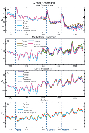
Figure 3.17. Observed surface and upper-air temperature anomalies (°C). (A) Lower stratospheric T4, (B) Tropospheric T2, (C) Lower tropospheric T2LT,from UAH, RSS and VG2 MSU satellite analyses and UKMO HadAT2 and NOAA RATPAC radiosonde observations; and (D) Surface records from NOAA, NASA/GISS and UKMO/CRU (HadCRUT2v). All time series are monthly mean anomalies relative to the period 1979 to 1997 smoothed with a seven-month running mean filter. Major volcanic eruptions are indicated by vertical blue dashed lines. Adapted from Karl et al. 2006 [NPR, PoC, SRC] ).
By differencing T2 measurements made at different slant angles, the UAH group produced an updated data record weighted for the lower and mid troposphere, T2LT ( Christy et al., 2003 [MoS, SRC] ). This retrieval also has the effect of removing the stratospheric influence on long-term trends, but its uncertainties are augmented by the need to compensate for orbital decay and by computing a small residual from two large values ( Wentz and Schabel, 1998 [JoC] ). T2LT retrievals include a large signal from the surface and so are adversely affected by changes in surface emissivity, including changes in sea ice cover ( Swanson, 2003 [JoC] Fu and Johanson 2005 [JoC] ) found that the T2LT trends were physically inconsistent compared with those of the surface, T2 and T4, even if taken from the UAH record. They also showed that the large trend bias is mainly attributed to the periods when a satellite had substantial drifts in local equator crossing time that caused large changes in calibration target temperatures and large diurnal drifts. Mears and Wentz 2005 [NPR, SRC] ) further found that the adjustments for diurnal cycle required from satellite drift had the wrong sign in the UAH record in the tropics. Corrections have been made (version 5.2; Christy and Spencer, 2005 [NPR, SRC] ) and are reflected in Figure 3.18 ,but the trend in the tropics is still smaller for most periods than both those in the troposphere (using T2 and T4) and those at the surface. Mears and Wentz 2005 [NPR, SRC] ) computed their own alternative T2LT record and found a T2LT trend nearly 0.1°C per decade larger than the revised UAH trend. After 1987, when MSU channel 3 became available, Fu and Johanson 2005 [JoC] ), using RSS data, found a systematic trend of increasing temperature with altitude throughout the tropics.
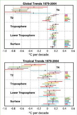
Figure 3.18. Linear temperature trends (°C per decade) for 1979 to 2004 for the globe (top) and tropics (20°N to 20°S; bottom) for the MSU channels T4 (top panel) and T2 (second panel) or equivalent for radiosondes and reanalyses; for the troposphere (third panel) based on T2 with T4 used to statistically remove stratospheric influences ( Fu et al., 2004a [JoC] ); for the lower troposphere (fourth panel) based on the UAH retrieval profile; and for the surface (bottom panel). Surface records are from NOAA/NCDC (green), NASA/GISS (blue) and HadCRUT2v (light blue). Satellite records are from UAH (orange), RSS (dark red) and VG2 (magenta); radiosonde-based records are from NOAA RATPAC (brown) and HadAT2 (light green); and atmospheric reanalyses are from NRA (red) and ERA-40 (cyan). The error bars are 5 to 95% confidence limits associated with sampling a finite record with an allowance for autocorrelation. Where the confidence limits exceed –1, the values are truncated. ERA-40 trends are only for 1979 to August 2002 . Data from Karl et al. 2006 [NPR, PoC, SRC] ; D. Seidel courtesy of J. Lanzante; and J. Christy).
Comparisons of tropospheric radiosonde station data with collocated satellite data ( Christy and Norris, 2004 [JoC, SRC] ) show considerable scatter, and root mean square differences between UAH satellite data and radiosondes are substantial ( Hurrell et al., 2000 [JoC, SRC] ). Although Christy and Norris 2004 [JoC, SRC] ) found good agreement between median radiosonde temperature trends and UAH trends, comparisons are more likely to be biased by spurious cooling than by spurious warming in unhomogenised ( Sherwood et al., 2005 [JoC, SRC] ) and even homogenised ( Randel and Wu, 2006 [JoC] ) radiosonde data (see Section 3.4.1.1 and Appendix 3.B.5.1). In the stratosphere, radiosonde trends are more negative than both MSU retrievals, especially when compared with RSS, and this is very likely due to changes in sondes and their processing for radiation corrections ( Randel and Wu, 2006 [JoC] ).
Geographical patterns of the linear trend in tropospheric temperature from 1979 to 2004 ( Figure 3.19 )are qualitatively similar in the RSS and UAH MSU data sets. Both show coherent warming over most of the NH, but UAH shows cooling over parts of the tropical Pacific and tropospheric temperature trends differ south of 45°S where UAH indicate more cooling than RSS.
Figure 3.19. Linear tropospheric temperature trends (°C per decade) for 1979 to 2005 from RSS (based on T2 and T4 adjusted as in Fu et al., 2004a [JoC] ). Courtesy Q. Fu.
3.4.1.3 Reanalyses
Acomprehensive global reanalysis completed since the TAR, ERA-40 ( Uppala et al., 2005 [JoC, SRC] ), extends from September 1957 to August 2002 . Reanalysis is designed to prevent changes in the analysis system from contaminating the climate record, as occurs with global analyses from operational numerical weather prediction, and it compensates for some but not all of the effects of changes in the observing system (see Appendix 3.B.5.4). Unlike the earlier NRA that assimilated satellite retrievals, ERA-40 assimilated bias-adjusted radiances including MSU data ( Harris and Kelly, 2001 [JoC] ; Uppala et al., 2005 [JoC, SRC] ), and the assimilation procedure itself accounts for orbital drift and change in satellite height – factors that have to be addressed in direct processing of MSU radiances for climate studies (e.g., Christy et al., 2003 [MoS, SRC] ; Mears et al., 2003 [JoC, SRC] ; Mears and Wentz, 2005 [NPR, SRC] ). Onboard calibration biases are treated indirectly via the influence of other data sets. Nonetheless, the veracity of low-frequency variability in atmospheric temperatures is compromised in ERA-40 by residual problems in bias corrections.
Trends and low-frequency variability in large-scale surface air temperature from ERA-40 and from the monthly climate station data analysed by Jones and Moberg 2003 [JoC, SRC] ) are in generally good agreement from the late 1970 s onwards (see also Section 3.2.2.1 ). Temperatures from ERA-40 vary quite coherently throughout the planetary boundary layer over this period, and earlier for regions with consistently good coverage from both surface and upper-air observations ( Simmons et al., 2004 [JoC, SRC] ).
Processed MSU records of layer temperature have been compared with equivalents derived from the ERA-40 analyses ( Santer et al., 2004 [PoC, JoC, ARC] ). The use of deep layers conceals disparate trends at adjacent tropospheric levels in ERA-40. Relatively cold tropospheric values before the satellite era arose from a combination of scarcity of radiosonde data over the extratropical SH and a cold bias of the assimilating model, giving a tropospheric warming trend that is clearly too large when taken over the full period of the reanalysis ( Bengtsson et al., 2004 [JoC, ARC] ; Simmons et al., 2004 [JoC, SRC] ; Karl et al., 2006 [NPR, PoC, SRC] ). ERA-40 also exhibits a middle-tropospheric cooling over most of the tropics and subtropics since the 1970 s that is certainly too strong owing to a warm bias in the analyses for the early satellite years.
Tropospheric patterns of trends from ERA-40 are similar to Figure 3.19 ,with coherent warming over the NH, although with discrepancies south of 45°S. These differences are not fully understood, although the treatment of surface emissivity anomalies over snow- and ice-covered surfaces may contribute ( Swanson, 2003 [JoC] ). At high southern latitudes, ERA-40 shows strong positive temperature trends in JJA in the period 1979 to 2001, in good accord with antarctic radiosonde data ( Turner et al., 2006 [JoC] ). The large-scale patterns of stratospheric cooling are similar in ERA-40 and the MSU data sets ( Santer et al., 2004 [PoC, JoC, ARC] ). However, the ERA-40 analyses in the lower stratosphere are biased cold relative to radiosonde data in the early satellite years, reducing downward trends. Section 3.5 relates the trends to atmospheric circulation changes.
3.4.1.4 The Tropopause
The tropopause marks the division between the troposphere and stratosphere and generally a minimum in the vertical profile of temperature. The height of the tropopause is affected by the heat balance of both the troposphere and the stratosphere. For example, when the stratosphere warms owing to absorption of radiation by volcanic aerosol, the tropopause is lowered. Conversely, a warming of the troposphere raises the tropopause, as does a cooling of the stratosphere. The latter is expected as a result of increasing greenhouse gas concentrations and stratospheric ozone depletion. Accordingly, changes in the height of the tropopause provide a sensitive indicator of human effects on climate. Inaccuracies and spurious trends in NRA preclude their use in determining tropopause trends ( Randel et al., 2000 [JoC] ) although they were found useful for interannual variability. Over 1979 to 2001, tropopause height increased by nearly 200 m (as a global average) in ERA-40, partly due to tropospheric warming plus stratospheric cooling ( Santer et al., 2004 [PoC, JoC, ARC] ). Atmospheric temperature changes in the UAH and RSS satellite MSU data sets (see Section 3.4.1.2 )were found to be more highly correlated with changes in ERA-40 than with those in NRA, illustrating the improved quality of ERA-40 and satellite data. The Santer et al. 2004 [PoC, JoC, ARC] ) results provide support for warming of the troposphere and cooling of the lower stratosphere over the last four decades of the 20th century, and indicate that both of these changes in atmospheric temperature have contributed to an overall increase in tropopause height. The radiosonde-based analyses of Randel et al. 2000 [JoC] Seidel et al. 2001 [JoC, ARC] and Highwood et al. 2000 [JoC, SRC] ) also show increases in tropical tropopause height.
3.4.1.5 Synthesis and Comparison with the Surface Temperatures
Figure 3.17 presents the radiosonde and satellite global time series and Figure 3.18 gives a summary of the linear trends for 1979 to 2004 for global and tropical (20°N to 20°S) averages. Values at the surface are from NOAA (NCDC), NASA (GISS), UKMO/CRU (HadCRUT2v) and the NRA and ERA-40 reanalyses. Trends aloft are for the lower troposphere corresponding to T2LT,T2, T4 and also the linear combination of T2 and T4 to better depict the entire troposphere as given by Fu et al. 2004a [JoC] ). In addition to the reanalyses, the results from the satellite-based methods from UAH, RSS and VG2 are given along with radiosonde estimates from HadAT2 and RATPAC. The ERA-40 trends only extend through August 2002, and VG2 is available only for T2. The error bars plotted here are 5 to 95% confidence limits associated with sampling a finite record where an allowance has been made for temporal autocorrelation in computing degrees of freedom( Appendix 3.A ). However, the error bars do not include spatial sampling uncertainty, which increases the noise variance. Noise typically cuts down on temporal autocorrelation and reduces the temporal sampling error bars, which is why the RATPAC error bars are often smaller than the rest. Other sources of ‘structural’ and ‘internal’ errors of order 0.08°C for 5 to 95% levels ( Mears and Wentz, 2005 [NPR, SRC] ; see Appendix 3.B.5) are also not explicitly accounted for here. Structural uncertainties and parametric errors ( Thorne et al., 2005b [PoC, JoC, SRC] ) reflect divergence between different data sets after the common climate variability has been accounted for and are better illustrated by use of difference time series, as seen for instance in T2 for RSS vs. UAH in Fu and Johanson 2005 [JoC] ; see also Karl et al., 2006 [NPR, PoC, SRC] ).
From Figure 3.17 the first dominant impression is that overall, the records agree remarkably well, especially in the timing and amplitude of interannual variations. This is especially true at the surface, and even the tropospheric records from the two radiosonde data sets agree reasonably well, although HadAT2 has lower values in the 1970 s. In the lower stratosphere, all records replicate the dominant variations and the pulses of warming following the volcanic eruptions indicated in the figure. The sonde records differ prior to 1963 in the lower stratosphere when fewer observations were available, and differences also emerge among all data sets after about 1992, with the sonde values lower than the satellite temperatures. The focus on linear trends tends to emphasize these relatively small differences.
Alinear trend over the long term is often not a very good approximation of what has occurred ( Seidel and Lanzante, 2004 [JoC, SRC] ; Thorne et al., 2005a [PoC, JoC, SRC] ,b); alternative interpretations are to factor in the abrupt 1976 – 1977 climate regime shift ( Trenberth, 1990 [PoC, JoC, SRC] ) and episodic stratospheric warming and tropospheric cooling for the two years following major volcanic eruptions. Hence, the confidence limits for linear trends( Figure 3.18 )are very large in the lower stratosphere owing to the presence of the large warming perturbations from volcanic eruptions. In the troposphere, the confidence limits are much wider in the tropics than globally, reflecting the strong interannual variability associated with ENSO.
Radiosonde, satellite observations and reanalyses agree that there has been global stratospheric cooling since 1979 (Figures 3.17 and 3.18 ), although radiosondes almost certainly still overestimate the cooling owing to residual effects of changes in instruments and processing (such as for radiation corrections; Lanzante et al., 2003b [JoC, SRC] ; Sherwood et al., 2005 [JoC, SRC] ; Randel and Wu, 2006 [JoC] ) and possibly increased sampling of cold conditions owing to stronger balloons ( Parker and Cox, 1995 [JoC] ). As the stratosphere is cooling and T2 has a 15% signal from there, it is virtually certain that the troposphere must be warming at a significantly greater rate than indicated by T2 alone. Thus, the tropospheric record adjusted for the stratospheric contribution to T2 has warmed more than T2 in every case. The differences range from 0.06°C per decade for ERA-40 to 0.09°C per decade for both radiosonde and NRA data sets. For UAH and RSS the difference is 0.07°C per decade.
The weakest tropospheric trends occur for NRA. However, unlike ERA-40, the NRA did not allow for changes in greenhouse gas increases over the record ( Trenberth, 2004 [PoC, JoC, SRC] ), resulting in errors in radiative forcing and in satellite retrievals in the infrared and making trends unreliable ( Randel et al., 2000 [JoC] ); indeed, upward trends at high surface mountain stations are stronger than NRA free-atmosphere temperatures at nearby locations ( Pepin and Seidel, 2005 [JoC] ). The records suggest that since 1979, the global and tropical tropospheric trends are similar to those at the surface although RSS, and by inference VG2, indicate greater tropospheric than surface warming. The reverse is indicated by the UAH and the radiosonde record although these data are subject to significant imperfections discussed above. Amplification occurs in the tropics for the RSS fields, especially after 1987 when there are increasing trends with altitude throughout the troposphere based on T2, T3 and T4 ( Fu and Johanson, 2005 [JoC] ). In the tropics, the theoretically expected amplification of temperature perturbations with height is borne out by interannual fluctuations (ENSO) in radiosonde, RSS, UAH and model data ( Santer et al., 2005 [PoC, JoC, ARC] ), but it is not borne out in the trends of the radiosonde records and UAH data.
The global mean trends since 1979 disguise many regional differences. In particular, in winter much larger temperature trends are present at the surface over northern continents than at higher levels ( Karl et al., 2006 [NPR, PoC, SRC] ) (see Figures 3.9 and 3.10 ; FAQ 3.1 ,Figure 1). These are associated with weakening of shallow winter temperature inversions and the strong stable surface layers that have little signature in the main troposphere. Such changes are related to changes in surface winds and atmospheric circulation (see Section 3.6.4 ).
In summary, for the period since 1958, overall global and tropical tropospheric warming estimated from radiosondes has slightly exceeded surface warming( Figure 3.17 and Karl et al., 2006 [NPR, PoC, SRC] ). The climate shift of 1976 appeared to yield greater tropospheric than surface warming( Figure 3.17 ); such climate variations make differences between the surface and tropospheric temperature trends since 1979 unsurprising. After 1979, there has also been global and tropical tropospheric warming; however, it is uncertain whether tropospheric warming has exceeded that at the surface because the spread of trends among tropospheric data sets encompasses the surface warming trend. The range (due to different data sets, but not including the reanalyses) of global surface warming since 1979 from Figure 3.18 is 0.16°C to 0.18°C per decade compared to 0.12°C to 0.19°C per decade for MSU estimates of tropospheric temperatures. A further complexity is that surface trends have been greater over land than over ocean. Substantial cooling has occurred in the lower stratosphere. Compensation for the effects of stratospheric cooling trends on the T2 record (a cooling of about 0.08°C per decade) has been an important development. However, a linear trend is a poor fit to the data in the stratosphere and the tropics at all levels. The overall global variability is well replicated by all records, although small relative trends exacerbate the differences between records. Inadequacies in the observations and analytical methods result in structural uncertainties that still contribute to the differences between surface and tropospheric temperature trends, and revisions continue to be made. Changes in the height of the tropopause since 1979 are consistent with overall tropospheric warming as well as stratospheric cooling.
3.4.2 Water Vapour
Water vapour is a key climate variable. In the lower troposphere, condensation of water vapour into precipitation provides latent heating which dominates the structure of tropospheric diabatic heating ( Trenberth and Stepaniak, 2003a [PoC, JoC, SRC] ,b). Water vapour is also the most important gaseous source of infrared opacity in the atmosphere, accounting for about 60% of the natural greenhouse effect for clear skies ( Kiehl and Trenberth, 1997 [PoC, JoC, SRC] ), and provides the largest positive feedback in model projections of climate change ( Held and Soden, 2000 [ARC] ).
Water vapour at the land surface has been measured since the late 19th century, but only observations made since the 1950 s have been compiled into a database suitable for climate studies. The concentration of surface water vapour is typically reported as the vapour pressure, dew point temperature or relative humidity. Using physical relationships, it is possible to convert from one to the other, but the conversions are exact only for instantaneous values. As the relationships are nonlinearly related to air temperature, errors accumulate as data are averaged to daily and monthly periods. Slightly more comprehensive data exist for oceanic areas, where the dew point temperature is included as part of the ICOADS database, but few analyses have taken place for periods before the 1950 s.
The network of radiosonde measurements provides the longest record of water vapour measurements in the atmosphere, dating back to the mid- 1940 s. However, early radiosonde sensors suffered from significant measurement biases, particularly for the upper troposphere, and changes in instrumentation with time often lead to artificial discontinuities in the data record (e.g., see Elliott et al., 2002 [JoC] ). Consequently, most of the analysis of radiosonde humidity has focused on trends for altitudes below 500 hPa and is restricted to those stations and periods for which stable instrumentation and reliable moisture soundings are available.
Additional information on water vapour can be obtained from satellite observations and reanalysis products. Satellite observations provide near-global coverage and thus represent an important source of information over the oceans, where radiosonde observations are scarce, and in the upper troposphere, where radiosonde sensors are often unreliable.
3.4.2.1 Surface and Lower-Tropospheric Water Vapour
Boundary layer moisture strongly determines the longwave (LW) radiative flux from the atmosphere to the surface. It also accounts for a significant proportion of the direct absorption of solar radiation by the atmosphere. The TAR reported widespread increases in surface water vapour in the NH. The overall sign of these trends has been confirmed from analysis of specific humidity over the USA ( Robinson, 2000 [JoC] ) and over China from 1951 to 1994 ( (Wang and Gaffen, 2001 ) ), particularly for observations made at night. Differences in the spatial, seasonal and diurnal patterns of these changes were found with strong sensitivity of the results to the network choice. Philipona et al. 2004 [JoC, MoS] ) inferred rapid increases in surface water vapour over central Europe from cloud-cleared LW radiative flux measured over the period 1995 to 2003 . Subsequent analyses ( Philipona et al., 2005 [JoC, MoS] ) confirmed that changes in integrated water vapour for this region are strongly coupled to the surface temperature, with regions of warming experiencing increasing moisture and regions of cooling experiencing decreasing moisture. For central Europe, Auer et al. 2007 [JoC, ARC, 2007] ) demonstrated increasing moisture trends. Their vapour pressure series from the Greater Alpine Region closely follow the decadal- to centennial-scale warming at both urban lowland and rural summit sites. In Canada, van Wijngaarden and Vincent 2005 [JoC] ) found a decrease in relative humidity of several percent in the spring for 75 stations, after correcting for instrumentation changes, but little change in relative humidity elsewhere or for other seasons. Ishii et al. 2005 [JoC, SRC] ) reported that globally averaged dew points over the ocean have risen by about 0.25°C between 1950 and 2000 . Increasing extremes in summer dew points, and increased humidity during summer heat waves, were found at three stations in northeastern Illinois ( Sparks et al., 2002 [JoC] ;( Changnon et al., 2003 ) ) and attributed in part to changes in agricultural practices in the region.
Dai 2006 [Ambiguous] ) analysed near-global (60°S–75°N) synoptic data for 1976 to 2005 from ships and buoys and more than 15,000 land stations for specific humidity, temperature and relative humidity. Nighttime relative humidity was found to be greater than daytime by 2 to 15% over most land areas, as temperatures undergo a diurnal cycle, while moisture does not change much. The global trends of near-surface relative humidity are very small. Trends in specific humidity tend to follow surface temperature trends with a global average increase of 0.06 g kg–1 per decade ( 1976 – 2004 ). The rise in specific humidity corresponds to about 4.9% per 1°C warming over the globe. Over the ocean, the observed surface specific humidity increases at 5.7% per 1°C warming, which is consistent with a constant relative humidity. Over land, the rate of increase is slightly smaller (4.3% per 1°C), suggesting a modest reduction in relative humidity as temperatures increase, as expected in water-limited regions.
For the lower troposphere, water vapour information has been available from the TOVS since 1979 and from the Scanning Multichannel Microwave Radiometer (SMMR) from 1979 to 1984 . However, the main improvement occurred with the introduction of the Special Sensor Microwave/Imager (SSM/I) in mid- 1987 ( Wentz and Schabel, 2000 [JoC] ). Retrievals of column-integrated water vapour from SSM/I are generally regarded as providing the most reliable measurements of lower-tropospheric water vapour over the oceans, although issues pertaining to the merging of records from successive satellites do arise ( Trenberth et al., 2005a [PoC, JoC, SRC] ; Sohn and Smith, 2003 [JoC] ).
Significant interannual variability of column-integrated water vapour has been observed using TOVS, SMMR and SSM/I data. In particular, column water vapour over the tropical oceans increased by 1 to 2 mm during the 1982 – 1983, 1986 – 1987 and 1997 – 1998 El Niño events ( Soden and Schroeder, 2000 [JoC, MoS, ARC] ; Allan et al., 2003 [JoC, MoS] ; Trenberth et al., 2005a [PoC, JoC, SRC] ) and decreased by a smaller magnitude in response to global cooling following the eruption of Mt. Pinatubo in 1991 ( Soden et al., 2002 [JoC, ARC] ; Trenberth and Smith, 2005 [PoC, JoC, SRC] ; see also Section 8.6.3.1 ). The linear trend based on monthly SSM/I data over the oceans was 1.2% per decade (0.40 ± 0.09 mm per decade) for 1988 to 2004 ( Figure 3.20 ). Since the trends are similar in magnitude to the interannual variability, it is likely that the latter affects the magnitude of the linear trends. The trends are overwhelmingly positive in spatial structure, but also suggestive of an ENSO influence. As noted by Trenberth et al. 2005a [PoC, JoC, SRC] ), most of the patterns associated with the interannual variability and linear trends can be reproduced from the observed SST changes over this period by assuming a constant relative humidity increase in water vapour mixing ratio. Given observed SST increases, this implies an overall increase in water vapour of order 5% over the 20th century and about 4% since 1970 .
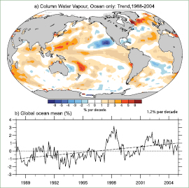
Figure 3.20. Linear trends in precipitable water (total column water vapour) in % per decade (top) and monthly time series of anomalies relative to the 1988 to 2004 period in % over the global ocean plus linear trend (bottom), from RSS SSM/I (updated from Trenberth et al., 2005a [PoC, JoC, SRC] ).
An independent check on globally vertically integrated water vapour amounts is whether the change in water vapour mass is reflected in the surface pressure field, as this is the only significant influence on the global atmospheric mass to within measurement accuracies. As Trenberth and Smith 2005 [PoC, JoC, SRC] ) showed, such checks indicate considerable problems prior to 1979 in reanalyses, but results are in better agreement thereafter for ERA-40. Evaluations of column integrated water vapour from the NASA Water Vapor Project (NVAP; Randel et al., 1996 [JoC] ), and reanalysis data sets from NRA, NCEP-2 and ERA-15/ERA-40 (see Appendix 3.B.5.4) reveal several deficiencies and spurious trends, which limit their utility for climate monitoring ( Zveryaev and Chu, 2003 [JoC, MoS] ; Trenberth et al., 2005a [PoC, JoC, SRC] ; Uppala et al., 2005 [JoC, SRC] ). The spatial distributions, trends and interannual variability of water vapour over the tropical oceans are not always well reproduced by reanalyses, even after the 1970 s ( Allan et al., 2002 [Ambiguous] , 2004; Trenberth et al., 2005a [PoC, JoC, SRC] ).
To summarise, global, local and regional studies all indicate increases in moisture in the atmosphere near the surface, but highlight differences between regions and between day and night. Satellite observations of oceanic lower-tropospheric water vapour reveal substantial variability during the last two decades. This variability is closely tied to changes in surface temperatures, with the water vapour mass changing at roughly the same rate at which the saturated vapour pressure does. A significant upward trend is observed over the global oceans and some NH land areas, although the calculated trend is likely influenced by large interannual variability in the record.
3.4.2.2 Upper-Tropospheric Water Vapour
Water vapour in the middle and upper troposphere accounts for a large part of the atmospheric greenhouse effect and is believed to be an important amplifier of climate change ( Held and Soden, 2000 [ARC] ). Changes in upper-tropospheric water vapour in response to a warming climate have been the subject of significant debate.
Due to instrumental limitations, long-term changes in water vapour in the upper troposphere are difficult to assess. ( Wang et al. 2001 ) ) found an increasing trend of 1 to 5% per decade in relative humidity during 1976 to 1995, with the largest increases in the upper troposphere, using 17 radiosonde stations in the tropical west Pacific. Conversely, a combination of Microwave Limb Sounder (MLS) and Halogen Occultation Experiment (HALOE) measurements at 215 hPa suggested increases in water vapour with increasing temperature ( Minschwaner and Dessler, 2004 [JoC, MoS] ) on interannual time scales, but at a rate smaller than expected from constant relative humidity.
( Maistrova et al. 2003 ) ) reported an increase in specific humidity at 850 hPa and a decrease from 700 to 300 hPa for 1959 to 2000 in the Arctic, based on data from ships and temporary stations as well as permanent stations. In general, the radiosonde trends are highly suspect owing to the poor quality of, and changes over time in, the humidity sensors (e.g., ( Wang et al., 2002a ) ). Comparisons of water vapour sensors during recent intensive field campaigns have produced a renewed appreciation of random and systematic errors in radiosonde measurements of upper-tropospheric water vapour and of the difficulty in developing accurate corrections for these measurements ( Guichard et al., 2000 [JoC] ; Revercombe et al., 2003 [JoC, MoS] ;( Turner et al., 2003; ) Wang et al., 2003 [JoC] ;( Miloshevich et al., 2004; ) Soden et al., 2004 [JoC, ARC] ).
Information on the decadal variability of upper-tropospheric relative humidity is now provided by 6.7 µm thermal radiance measurements from Meteosat ( Picon et al., 2003 [JoC] ) and the High-resolution Infrared Radiation Sounder (HIRS) series of instruments flying on NOAA operational polar-orbiting satellites ( (Bates and Jackson, 2001; ) Soden et al., 2005 [JoC, ARC] ). These products rely on the merging of many different satellites to ensure uniform calibration. The HIRS channel 12 (T12) data have been most extensively analysed for variability and show linear trends in relative humidity of order ±1% per decade at various latitudes ( (Bates and Jackson, 2001 ) ), but these trends are difficult to separate from larger interannual fluctuations due to ENSO ( McCarthy and Toumi, 2004 [JoC] ) and are negligible when averaging over the tropical oceans ( Allan et al., 2003 [JoC, MoS] ).
In the absence of large changes in relative humidity, the observed warming of the troposphere (see Section 3.4.1 )implies that the specific humidity in the upper troposphere should have increased. As the upper troposphere moistens, the emission level for T12 increases due to the increasing opacity of water vapour along the satellite line of sight. In contrast, the emission level for the MSU T2 remains constant because it depends primarily on the concentration of oxygen, which does not vary by any appreciable amount. Therefore, if the atmosphere moistens, the brightness temperature difference (T2 − T12) will increase over time due to the divergence of their emission levels ( Soden et al., 2005 [JoC, ARC] ). This radiative signature of upper-tropospheric moistening is evident in the positive trends of T2 − T12 for the period 1982 to 2004 ( Figure 3.21 ). If the specific humidity in the upper troposphere had not increased over this period, the emission level for T12 would have remained unchanged and T2 − T12 would show little trend over this period (dashed line in Figure 3.21 ).
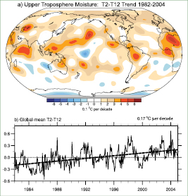
Figure 3.21. The radiative signature of upper-tropospheric moistening is given by upward linear trends in T2−T12 for 1982 to 2004 (0.1 ºC per decade; top) and monthly time series of the global-mean (80°N to 80°S) anomalies relative to 1982 to 2004 (ºC) and linear trend (dashed; bottom). Data are from the RSS T2 and HIRS T12 ( Soden et al., 2005 [JoC, ARC] ). The map is smoothed to spectral truncation T31 resolution.
Clear-sky outgoing longwave radiation (OLR) is also highly sensitive to upper-tropospheric water vapour and a number of scanning instruments have made well-calibrated but non-overlapping measurements since 1985 (see Section 3.4.3 ). Over this period, the small changes in clear-sky OLR can be explained by the observed temperature changes while maintaining a constant relative humidity ( Wong et al., 2000 [JoC, SRC] ; Allan and Slingo, 2002 [JoC, MoS] ) and changes in well-mixed greenhouse gases ( Allan et al., 2003 [JoC, MoS] ). This again implies a positive relationship between specific humidity and temperature in the upper troposphere.
To summarise, the available data do not indicate a detectable trend in upper-tropospheric relative humidity. However, there is now evidence for global increases in upper-tropospheric specific humidity over the past two decades, which is consistent with the observed increases in tropospheric temperatures and the absence of any change in relative humidity.
3.4.2.4 Stratospheric Water Vapour
The TAR noted an apparent increase of roughly 1% yr–1 in stratospheric water vapour content (~0.05 ppm yr–1)during the last half of the 20th century ( Kley et al., 2000 [NPR] ; Rosenlof et al., 2001 [JoC, SRC] ). This was based on data taken at mid-latitudes, and from multiple instruments. However, the longest series of data come from just two locations in North America with no temporal overlap. The combination of measurement uncertainties and relatively large variability on time scales from months to years warrants some caution when interpreting the longer-term trends ( Kley et al., 2000 [NPR] ; Fueglistaler and Haynes, 2005 [JoC] ). The moistening is more convincingly documented during the 1980 s and most of the 1990 s than earlier, due to a longer continuous record (the NOAA Climate Monitoring and Diagnostics Laboratory (CMDL) frost-point balloon record from Boulder, Colorado; Oltmans et al., 2000 [JoC] ) and the availability of satellite observations during much of this period. However, discrepancies between satellite- and balloon-measured variations are apparent at decadal time scales, largely over the latter half of the 1990 s ( Randel et al., 2004a [JoC] ).
An increase in stratospheric water vapour has important radiative and chemical consequences (see also Section 2.3.8 ). These may include a contribution to the recent observed cooling of the lower stratosphere and/or warming of the surface ( Forster and Shine, 1999 [JoC] , 2002; Smith et al., 2001 [JoC, MoS, ARC] ), although the exact magnitude is difficult to quantify ( Oinas et al., 2001 [JoC] ; Forster and Shine, 2002 [JoC] ). Some efforts to reconcile observed rates of cooling in the stratosphere with those expected based on observed changes in ozone and carbon dioxide (CO2)since 1979 ( Langematz et al., 2003 [JoC] ; Shine et al., 2003 [JoC, MoS] ) have found discrepancies in the lower stratosphere consistent with an additional cooling effect of a stratospheric water vapour increase. However, Shine et al. 2003 [JoC, MoS] ) noted that because the water vapour observations over the period of consideration are not global in extent, significant uncertainties remain as to whether radiative effects of a water vapour change are a significant contributor to the stratospheric temperature changes. Moreover, other studies which account for uncertainties in the ozone profiles and temperature trends, and natural variability, can reconcile the observed stratospheric temperature changes without the need for sizable water vapour changes ( Ramaswamy and Schwarzkopf, 2002 [JoC, ARC] ; Schwarzkopf and Ramaswamy, 2002 [JoC, ARC] ).
Although methane oxidation is a major source of water in the stratosphere, and has been increasing over the industrial period, the noted stratospheric trend in water vapour is too large to attribute to methane oxidation alone ( Kley et al., 2000 [NPR] ; Oltmans et al., 2000 [JoC] ). Therefore, other contributors to an increase in stratospheric water vapour are under active investigation. It is likely that different mechanisms are affecting water vapour trends at different altitudes. Aviation emits a small but potentially significant amount of water vapour directly into the stratosphere ( IPCC, 1999 [NPR] ). Several indirect mechanisms have also been considered including: a) volcanic eruptions ( Considine et al., 2001 [JoC, MoS] ; Joshi and Shine, 2003 [JoC] ); b) biomass-burning aerosol ( Sherwood, 2002 [JoC, SRC] ; Andreae et al., 2004 [JoC] ); c) tropospheric sulphur dioxide ( Notholt et al., 2005 [JoC] ); and d) changes to methane oxidation rates from changes in stratospheric chlorine, ozone and the hydroxyl radical ( (Röckmann et al., 2004 ) ). Other proposed mechanisms relate to changes in tropopause temperatures or circulation ( Stuber et al., 2001 [JoC, ARC] ; Zhou et al., 2001 [JoC, ARC] ; Rosenlof, 2002 [SRC] ; Nedoluha et al., 2003 [JoC] ; Dessler and Sherwood, 2004 [JoC, SRC] ; Fueglistaler et al., 2004 [JoC] ;( Roscoe, 2004 ) ).
It has been assumed that temperatures near the tropical tropopause control stratospheric water vapour according to equilibrium thermodynamics, importing more water vapour into the stratosphere when temperatures are warmer. However, tropical tropopause temperatures have cooled slightly over the period of the stratospheric water vapour increase (see Section 3.4.1 ;Seidel et al., 2001 [JoC, ARC] ; Zhou et al, 2001 [JoC, ARC] ). This makes the mid-latitude lower-stratospheric increases harder to explain ( Fueglistaler and Haynes, 2005 [JoC] ). Satellite observations ( Read et al., 2004 [JoC] ) show water vapour injected above the tropical tropopause by deep convective clouds, bypassing the traditional control point. Changes in the amount of condensate sublimating in this layer may have contributed to the upward trend, but to what degree is uncertain ( Sherwood, 2002 [JoC, SRC] ). Another suggested source for temperature-independent variability is changes in the efficiency with which air is circulated through the coldest regions before entering the stratosphere ( Hatsushika and Yamazaki, 2003 [JoC] ; Bonnazola and Haynes, 2004 [JoC] ; Dessler and Sherwood, 2004 [JoC, SRC] ; Fueglistaler et al., 2004 [JoC] ). However, it is not yet clear that a circulation-based mechanism can explain the observed trend ( Fueglistaler and Haynes, 2005 [JoC] ).
The TAR noted a stalling of the upward trend in water vapour during the last few years of observations available at that time. This change in behaviour has persisted, with a near-zero trend in stratospheric water vapour between 1996 and 2000 ( Nedoluha et al., 2003 [JoC] ; Randel et al., 2004a [JoC] ). The upward trend of methane is also smaller and is currently close to zero (see Section 2.3.2 ). Further, at the end of 2000 there was a dramatic drop in water vapour in the tropical lower stratosphere as observed by both satellite and CMDL balloon data ( Randel et al., 2004a [JoC] ). Temperatures observed near the tropical tropopause also dropped, but the processes producing the tropical tropopause cooling itself are currently not fully understood. The propagation of this recent decrease through the stratosphere should ensure flat or decreasing stratospheric moisture for at least the next few years.
To summarise, water vapour in the stratosphere has shown significant long-term variability and an apparent upward trend over the last half of the 20th century but with no further increases since 1996 . It does not appear that this behaviour is a straightforward consequence of known climate changes. Although ideas have been put forward, there is no consensus as to what caused either the upward trend or its recent disappearance.
3.4.3 Clouds
Clouds play an important role in regulating the flow of radiation at the top of the atmosphere and at the surface. They are also integral to the atmospheric hydrological cycle via their integral influence on the balance between radiative and latent heating. The response of cloud cover to increasing greenhouse gases currently represents the largest uncertainty in model predictions of climate sensitivity (see Chapter8 ). Surface observations made at weather stations and onboard ships, dating back over a century, provide the longest available records of cloud cover changes. Surface observers report the all-sky conditions, which include the sides as well as bottoms of clouds, but are unable to report upper-level clouds that may be obscured from the observer’s view. Although limited by potential inhomogeneities in observation times and methodology, the surface-observed cloud changes are often associated with physically consistent changes in correlative data, strengthening their credibility. Since the mid- 1990 s, especially in the USA and Canada, human observations at the surface have been widely replaced with automated ceilometer measurements, which measure only directly overhead low clouds rather than all-sky conditions. In contrast, satellites generally only observe the uppermost level of clouds and have difficulty detecting optically thin clouds. While satellite measurements do provide much better spatial and temporal sampling than can be obtained from the surface, their record is much shorter in length. These disparities in how cloud cover is observed contribute to the lack of consistency between surface- and satellite-measured changes in cloudiness. Condensation trails (‘contrails’) from aircraft exhaust may expand to form cirrus clouds and these and cosmic ray relations to clouds are addressed in Chapter2 .
3.4.3.1 Surface Cloud Observations
As noted in the TAR and extended with more recent studies, surface observations suggest increased total cloud cover since the middle of the last century over many continental regions including the USA ( Sun, 2003 [NPR, JoC] ; Groisman et al., 2004 [JoC, SRC] ; Dai et al., 2006 [Ambiguous] ), the former USSR ( Sun and Groisman, 2000 [JoC, SRC] ; Sun et al., 2001 [JoC, SRC] ), Western Europe, mid-latitude Canada, and Australia ( Henderson-Sellers, 1992 [ARC] ). This increasing cloudiness since 1950 is consistent with an increase in precipitation and a reduction in DTR ( Dai et al., 2006 [Ambiguous] ). However, decreasing cloudiness over this period has been reported over China ( Kaiser, 1998 [JoC] ), Italy ( Maugeri et al., 2001 [JoC] ) and over central Europe ( Auer et al., 2007 [JoC, ARC, 2007] ). If the analyses are restricted to after about 1971, changes in continental cloud cover become less coherent. For example, using a worldwide analysis of cloud data ( Hahn and Warren, 2003 [NPR, SRC] ; Minnis et al., 2004 [JoC] ) regional reductions were found since the early 1970 s over western Asia and Europe but increases over the USA.
Changes in total cloud cover along with an estimate of precipitation over global and hemispheric land (excluding North America) from 1976 to 2003 are shown in Figure 3.22 .During this period, secular trends over land are small. The small variability evident in land cloudiness appears to be correlated with precipitation changes, particularly in the SH( Figure 3.22 ). Note that surface observations from North America are excluded from this figure due to the declining number of human cloud observations since the early 1990 s over the USA and Canada, as human observers have been replaced with Automated Surface Observation Systems (ASOS) from which cloud amounts are less reliable and incompatible with previous records ( Dai et al., 2006 [Ambiguous] ). However, independent human observations from military stations suggest an increasing trend (~1.4% of sky per decade) in total cloud cover over the USA.
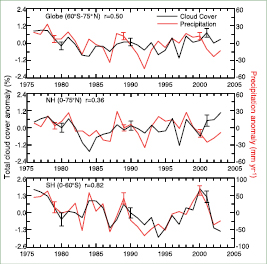
Figure 3.22. Annual total land (excluding the USA and Canada) cloud cover (black) and precipitation (red) anomalies from 1976 to 2003 over global (60°S–75°N), NH and SH regions, with the correlation coefficient (r) shown at the top. The cloud cover is derived by gridding and area-averaging synoptic observations and the precipitation is updated from Chen et al. 2002 [JoC] ). Typical 5 to 95% error bars for each decade are estimates using inter-grid-box variations (from Dai et al., 2006 [Ambiguous] ).
The TAR also noted multi-decadal trends in cloud cover over the ocean. An updated analysis of this information ( Norris, 2005a [JoC, MoS, SRC] ) documented substantial decadal variability and decreasing trends in upper-level cloud cover over mid- and low-latitude oceans since 1952 . However, there are no direct observations of upper-level clouds from the surface and instead Norris 2005a [JoC, MoS, SRC] ) infers them from reported total and low cloud cover assuming a random overlap. These results partially reverse the finding of increasing trends in mid-level cloud amount in the northern mid-latitude oceans that was reported in the TAR, although the new study does not distinguish between high and middle clouds. Norris 2005b [JoC, SRC] ) found that upper-level cloud cover had increased over the equatorial South Pacific between 1952 and 1997 and decreased over the adjacent subtropical regions, the tropical Western Pacific, and the equatorial Indian Ocean. This pattern is consistent with decadal changes in precipitation and atmospheric circulation over these regions noted in the TAR, which further supports their validity. Deser et al. 2004 [JoC, SRC] ) found similar spatial patterns in inter-decadal variations in total cloud cover, SST and precipitation over the tropical Pacific and Indian Oceans during 1900 to 1995 . In contrast, low-cloud cover increased over almost all of the tropical Indian and Pacific Oceans, but this increase bears little resemblance to changes in atmospheric circulation over this period, suggesting that it may be spurious ( Norris, 2005b [JoC, SRC] ). When averaged globally, oceanic cloud cover appears to have increased over the last 30 years or more (e.g., Ishii et al., 2005 [JoC, SRC] ).
During El Niño events, cloud cover generally decreases over land throughout much of the tropics and subtropics, but increases over the ocean in association with precipitation changes ( Curtis and Adler, 2003 [JoC, SRC] ). Multi-decadal variations are affected by the 1976 – 1977 climate shift ( Deser et al., 2004 [JoC, SRC] ), and these dominate the low-latitude trends from 1971 to 1996 found in Hahn and Warren 2003 [NPR, SRC] ).
3.4.3.2 Satellite Cloud Observations
Since the TAR, there has been considerable effort in the development and analysis of satellite data sets for documenting changes in global cloud cover over the past few decades. The most comprehensive cloud climatology is that of the International Satellite Cloud Climatology Project (ISCCP), begun in July 1983 . The ISCCP shows an increase in globally averaged total cloud cover of about 2% from 1983 to 1987, followed by a decline of about 4% from 1987 to 2001 ( Rossow and Dueñas, 2004 [JoC] Cess and Udelhofen 2003 [JoC] ) documented decreasing ISCCP total cloud cover in all latitude zones between 40°S and 40°N. Norris 2005a [JoC, MoS, SRC] ) found that both ISCCP and ship synoptic reports show consistent reductions in middle- or high-level cloud cover from the 1980 s to the 1990 s over low- and mid-latitude oceans. Minnis et al. 2004 [JoC] ) also found consistent trends in high-level cloud cover between ISCCP and surface observations over most areas, except for the North Pacific where they differed by almost 2% per decade. In addition, an analysis of Stratospheric Aerosol and Gas Experiment II (SAGE II) data revealed a decline in cloud frequency above 12 km between 1985 and 1998 ( Wang et al., 2002b [JoC] ) that is consistent with the decrease in upper-level cloud cover noted in ISCCP and ocean surface observations. The decline in upper-level cloud cover since 1987 may also be consistent with a decrease in reflected shortwave (SW) radiation during this period as measured by the Earth Radiation Budget Satellite (ERBS; see Section 3.4.4 ). Radiative transfer calculations, which use the ISCCP cloud properties as input, are able to independently reproduce the decadal changes in outgoing LW and reflected SW radiation reported by ERBS ( Zhang et al., 2004c [JoC, MoS] ).
Analyses of the spatial trends in ISCCP cloud cover reveal changing biases arising from changes in satellite view angle and coverage that affect the global mean anomaly time series ( Norris, 2000 [SRC] ; Dai et al., 2006 [Ambiguous] ). The ISCCP spurious variability may occur primarily in low-level clouds with the least optical thickness (the ISCCP ‘cumulus’ category; Norris, 2005a [JoC, MoS, SRC] ), due to discontinuities in satellite view angles associated with changes in satellites. Such biases likely contribute to ISCCP’s negative cloud cover trend, although their magnitude and impact on radiative flux calculations using ISCCP cloud data are not yet known. Additional artefacts, including radiometric noise, navigation and rectification errors are present in the ISCCP data ( Norris, 2000 [SRC] ), but the effects of known and unknown artefacts on ISCCP cloud and flux data have not yet been quantified.
Other satellite data sets show conflicting decadal changes in total cloud cover. For example, analysis of cloud cover changes from the HIRS shows a slight increase in cloud cover between 1985 and 2001 ( Wylie et al., 2005 [JoC] ). However, spurious changes have also been identified in the HIRS data set, which may affect its estimates of decadal variability. One important source of uncertainty results from the drift in Equatorial Crossing Time (ECT) of polar-orbiting satellite measurements (e.g., HIRS and the Advanced Very High Resolution Radiometer; AVHRR), which aliases the large diurnal cycle of clouds into spurious lower-frequency variations. After correcting for ECT drift and other small calibration errors in AVHRR measurements of cloudiness, Jacobowitz et al. 2003 [JoC] ) found essentially no trend in cloud cover for the tropics from 1981 to 2000 .
While the variability in surface-observed upper-level cloud cover has been shown to be consistent with that observed by ISCCP ( Norris, 2005a [JoC, MoS, SRC] ), the variability in total cloud cover is not, implying differences between ISCCP and surface-observed low cloud cover. Norris 2005a [JoC, MoS, SRC] ) shows that even after taking into account the difference between surface and satellite views of low-level clouds, the decadal changes between the ISCCP and surface data sets still disagree. The extent to which this results from differences in spatial and temporal sampling or differences in viewing perspective is unclear.
In summary, while there is some consistency between ISCCP, ERBS, SAGE II and surface observations of a reduction in high cloud cover during the 1990 s relative to the 1980 s, there are substantial uncertainties in decadal trends in all data sets and at present there is no clear consensus on changes in total cloudiness over decadal time scales.
3.4.4 Radiation
Measuring the radiation balance accurately is fundamental in quantifying the radiative forcing of the system as well as diagnosing the radiative properties of the atmosphere and surface, which are crucial for understanding radiative feedback processes. At the top of the atmosphere, satellites provide excellent spatial coverage but poorer temporal sampling. The reverse is true at the surface with only a limited number of high-quality point measurements but with excellent temporal coverage.
3.4.4.1 Top-of-Atmosphere Radiation
One important development since the TAR is the apparent unexpectedly large changes in tropical mean radiation flux reported by ERBS ( Wielicki et al., 2002a [JoC, SRC] ,b). It appears to be related in part to changes in the nature of tropical clouds ( Wielicki et al., 2002a [JoC, SRC] ), based on the smaller changes in the clear-sky component of the radiative fluxes ( Wong et al., 2000 [JoC, SRC] ; Allan and Slingo, 2002 [JoC, MoS] ), and appears to be statistically distinct from the spatial signals associated with ENSO ( Allan and Slingo, 2002 [JoC, MoS] ; Chen et al., 2002 [JoC] ). A recent reanalysis of the ERBS active-cavity broadband data corrects for a 20 km change in satellite altitude between 1985 and 1999 and changes in the SW filter dome ( Wong et al., 2006 [JoC, SRC] ). Based upon the revised (Edition 3_Rev1) ERBS record( Figure 3.23 ), outgoing LW radiation over the tropics appears to have increased by about 0.7 Wm–2 while the reflected SW radiation decreased by roughly 2.1 Wm–2 from the 1980 s to 1990 s( Table 3.5 ).
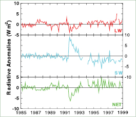
Figure 3.23. Tropical mean (20°S to 20°N) TOA flux anomalies from 1985 to 1999 (Wm–2)for LW, SW, and NET radiative fluxes [NET = −(LW + SW)]. Coloured lines are observations from ERBS Edition 3_Rev1 data from Wong et al. 2006 [JoC, SRC] ) updated from Wielicki et al. 2002a [JoC, SRC] ), including spacecraft altitude and SW dome transmission corrections.
These conclusions depend upon the calibration stability of the ERBS non-scanner record, which is affected by diurnal sampling issues, satellite altitude drifts and changes in calibration following a three-month period when the sensor was powered off ( Trenberth, 2002 [PoC, JoC, SRC] ). Moreover, rather than a trend, the reflected SW radiation change may stem mainly from a jump in late 1992 in the ERBS record that is also observed in the ISCCP (version FD) record ( Zhang et al., 2004c [JoC, MoS] ) but not in the AVHRR Pathfinder record ( Jacobowitz et al., 2003 [JoC] ). However, careful inspection of the sensor calibration revealed no known issues that can explain the decadal shift in the fluxes despite corrections to the ERBS time series relating to diurnal aliasing and satellite altitude changes ( Wielicki et al., 2002b [JoC, SRC] ; Wong et al., 2006 [JoC, SRC] ).
As noted in Section 3.4.3 ,the low-latitude changes in the radiation budget appear consistent with reduced cloud fraction from ISCCP. Detailed radiative transfer computations, using ISCCP cloud products along with additional global data sets, show broad agreement with the ERBS record of tropical radiative fluxes ( (Hatzianastassiou et al., 2004; ) Zhang et al., 2004c [JoC, MoS] ; Wong et al., 2006 [JoC, SRC] ). However, the decrease in reflected SW radiation from the 1980 s to the 1990 s may be inconsistent with the increase in total and low cloud cover over oceans reported by surface observations ( Norris, 2005a [JoC, MoS, SRC] ), which show increased low cloud occurrence. The degree of inconsistency, however, is difficult to ascertain without information on possible changes in low-level cloud albedo.
While the ERBS satellite provides the only continuous long-term top-of-atmosphere (TOA) flux record from broadband active-cavity instruments, narrow spectral band radiometers have made estimates of both reflected SW and outgoing LW radiation trends using regressions to broadband data, or using radiative transfer theory to estimate unmeasured portions of the spectrum of radiation. Table 3.5 shows the 1980 s to 1990 s TOA tropical mean flux changes for the ERBS Edition 3 data ( Wong et al., 2006 [JoC, SRC] ), the HIRS Pathfinder data ( Mehta and Susskind, 1999 [JoC] ), the AVHRR Pathfinder data ( Jacobowitz et al., 2003 [JoC] ) and the ISCCP FD data ( Zhang et al., 2004c [JoC, MoS] ).
The most accurate of the data sets in Table 3.5 is believed to be the ERBS Edition 3 Rev 1 active-cavity wide field of view data ( Wielicki et al., 2005 [JoC, SRC] ). The ERBS stability is estimated as better than 0.5 Wm–2 over the 1985 to 1999 period and the spatial and temporal sampling noise is less than 0.5 Wm–2 on annual time scales ( Wong et al., 2006 [JoC, SRC] ). The outgoing LW radiation changes from ERBS are similar to the decadal changes in the HIRS Pathfinder and ISCCP FD records, but disagree with the AVHRR Pathfinder data ( Wong et al., 2006 [JoC, SRC] ). The AVHRR Pathfinder data also do not support the TOA SW radiation trends. However, calibration issues, conversion from narrow to broadband, and satellite orbit changes are thought to render the AVHRR record less reliable for decadal changes compared to ERBS ( Wong et al., 2006 [JoC, SRC] ). Estimates of the stability of the ISCCP time series for long-term TOA flux records are 3 to 5 Wm–2 for SW radiative flux and 1 to 2 Wm–2 for LW radiative flux ( (Brest et al., 1997 ) ), although the time series agreement of the ISCCP and ERBS records are much closer than these estimated calibration drift uncertainties ( Zhang et al., 2004c [JoC, MoS] ).
Table 3.5. Top-of-atmosphere (TOA) radiative flux changes from the 1980 s to 1990 s (Wm–2). Values are given as tropical means (20°S to 20°N) for the 1994 to 1997 period minus the 1985 to 1989 period. Dashes are shown where no data are available. From Wong et al. 2006 [JoC, SRC] ).
| Radiative Flux Change (Wm–2) | |||
|---|---|---|---|
| Data Source | TOA LW | TOA SW | TOA Net |
| ERBS Edition 3 Rev 1 | 0.7 | –2.1 | 1.4 |
| HIRS Pathfinder | 0.2 | – | – |
| AVHRR Pathfinder | –1.4 | 0.7 | 0.7 |
| ISCCP FD | 0.5 | –2.4 | 1.8 |
The changes in SW radiation measured by ERBS Edition 3 Rev 1 are larger than the clear-sky flux changes due to humidity variations ( Wong et al., 2000 [JoC, SRC] ) or anthropogenic radiative forcing (see Chapter2 ). If correct, the large decrease in reflected SW radiation with little change in outgoing LW radiation implies a reduction in tropical low cloud cover over this period. However, specific information on cloud radiative forcing is not available from ERBS after 1989 and, as noted in Section 3.4.3 ,surface data sets suggest an increase in low cloud cover over this period.
Since most of the net tropical heating of 1.4 Wm–2 is a decrease in reflected SW radiative flux, the change implies a similar increase in solar insolation at the surface that, if unbalanced by other changes in surface fluxes, would increase the amount of ocean heat storage. Wong et al. 2006 [JoC, SRC] ) showed that the changes in global net radiation are consistent with a new ocean heat-storage data set from Willis et al. 2004 [JoC, ARC] ; see Chapter5 and Figure 5.1 ). Differences between the two data sets are roughly 0.4 Wm–2,in agreement with the estimated annual sampling noise in the ocean heat-storage data.
Using astronomical observations of visible wavelength solar photons reflected from parts of the Earth to the moon and then back to the Earth at a surface-based observatory, Pallé et al. 2004 [JoC] ) estimated a dramatic increase of Earth-reflected SW radiative flux of 5.5 Wm–2 over three years. This is unlikely to be real, as over the same time period ( 2000 – 2003 ), the Clouds and the Earth’s Radiant Energy System (CERES) broadband data indicate a decrease in SW radiative flux of almost 1 Wm–2,which is much smaller and the opposite sign ( Wielicki et al., 2005 [JoC, SRC] ). In addition, changes in ocean heat storage are more consistent with the CERES data than with the Earthshine indirect observation.
The only long-term time series ( 1979 – 2001 ) of energy divergence in the atmosphere ( Trenberth and Stepaniak, 2003b [PoC, JoC, SRC] ) are based on NRA, which, although not reliable for depicting trends, are reliable on interannual times scales for which they show substantial variability associated with ENSO. Analyses by Trenberth and Stepaniak 2003b [PoC, JoC, SRC] ) reveal more divergence of energy out of the deep tropics in the 1990 s compared with the 1980 s due to differences in ENSO, which may account for at least some of the changes discussed above.
In summary, although there is independent evidence for decadal changes in TOA radiative fluxes over the last two decades, the evidence is equivocal. Changes in the planetary and tropical TOA radiative fluxes are consistent with independent global ocean heat-storage data, and are expected to be dominated by changes in cloud radiative forcing. To the extent that they are real, they may simply reflect natural low-frequency variability of the climate system.
3.4.4.2 Surface Radiation
The energy balance at the surface requires net radiative heating to be balanced by turbulent energy fluxes and thus determines the evolution of surface temperature and the cycling of water, which are key parameters of climate change (see Box 7.1 ). In recent years, several studies have focused on observational evidence of changing surface radiative heating. Reliable SW radiative measurement networks have existed since the 1957 – 1958 International Geophysical Year.
Areduction in downward solar radiation (‘dimming’) of about 1.3% per decade or about 7 Wm–2 was observed from 1961 to 1990 at land stations around the world ( Gilgen et al., 1998 [JoC, MoS, ARC] ; Liepert, 2002 [JoC, SRC] ). Additional studies also found declines in surface solar radiation in the Arctic and Antarctic ( (Stanhill and Cohen, 2001 ) ) as well as at sites in the former Soviet Union ( Russak, 1990 [JoC] ; Abakumova et al., 1996 [JoC] ), around the Mediterranean Sea ( (Aksoy, 1997; ) ( Omran, 2000 ) ), China ( (Ren et al., 2005 ) ), the USA ( Liepert, 2002 [JoC, SRC] ) and southern Africa ( Power and Mills, 2005 [JoC] ( Stanhill and Cohen 2001 ) ) claim an overall globally averaged reduction of 2.7% per decade but used only 30 records. However, the stations where these analyses took place are quite limited in domain and dominated by large urban areas, and the dimming is much less at rural sites ( Alpert et al., 2005 [JoC] ) or even missing altogether over remote areas, except for identifiable effects of volcanic eruptions, such as Mt. Pinatubo in 1991 ( Schwartz, 2005 [JoC] ). At the majority of 421 analysed sites, the decline in surface solar radiation ended around 1990 and a recovery of about 6 Wm–2 occurred afterwards ( Wild et al., 2004 [JoC, ARC] ; 2005 ). The increase in surface solar radiation (‘brightening’) agrees with satellite and surface observations of reduced cloud cover ( Wang et al., 2002b [JoC] ; Wielicki et al., 2002a [JoC, SRC] ; Rossow and Dueñas, 2004 [JoC] ; Norris, 2005b [JoC, SRC] ; Pinker et al., 2005 [JoC] ), although there is evidence that some of these changes are spurious (see Section 3.4.3 ). In addition, the satellite-observed increase in surface radiation noted by Pinker et al. 2005 [JoC] ) occured primarily over ocean, whereas the increase observed by Wild et al. 2005 [JoC, ARC] ) was restricted to land stations.
Box 3.2: The Dimming of the Planet and Apparent Conflicts in Trends of Evaporation and Pan Evaporation
Several reports have defined the term ‘global dimming’ (e.g., Cohen et al., 2004 [JoC, SRC] ). This refers to a widespread reduction of solar radiation received at the surface of the Earth, at least up until about 1990 ( Wild et al., 2005 [JoC, ARC] ). However, recent studies ( Alpert et al., 2005 [JoC] ; Schwartz, 2005 [JoC] ) found that dimming is not global but is rather confined only to large urban areas. At the same time there is considerable confusion in the literature over conflicting trends in pan evaporation and actual evaporation ( Ohmura and Wild, 2002 [JoC, ARC] ; Roderick and Farquhar, 2002 [JoC] , 2004, 2005; Hobbins et al., 2004 [JoC] ; Wild et al., 2004 [JoC, ARC] , 2005 ) although the framework for explaining observed changes exists ( Brutsaert and Parlange, 1998 [JoC] ).
Surface evaporation, or more generally evapotranspiration, depends upon two key components. The first is available energy at the surface, especially solar radiation. The second is the availability of surface moisture, which is not an issue over oceans, but which is related to soil moisture amounts over land. Evaporation pans provide estimates of the potential evaporation that would occur if the surface were wet. Actual evaporation is generally not measured, except at isolated flux towers, but may be computed using bulk flux formulae or estimated as a residual from the surface moisture balance.
The evidence is strong that a key part of the solution to the paradox of conflicting trends in evaporation and pan evaporation lies in changes in the atmospheric circulation and the hydrological cycle. There has been an increase in clouds and precipitation, which reduce solar radiation available for actual and potential evapotranspiration but also increase soil moisture and make the actual evapotranspiration closer to the potential evapotranspiration. An increase in both clouds and precipitation has occurred over many parts of the land surface ( Dai et al., 1999 [PoC, JoC, SRC] , 2004a, 2006 ), although not in the tropics and subtropics (which dominate the global land mean; Section 3.3.2.2 ). This reduces solar radiation available for evapotranspiration, as observed since the late 1950 s or early 1960 s over the USA ( Liepert, 2002 [JoC, SRC] ), parts of Europe and Siberia ( Peterson et al., 1995 [JoC, SRC] ; Abakumova et al., 1996 [JoC] ), India ( Chattopadhyay and Hulme, 1997 [MoS] ), China ( Liu et al., 2004a [JoC] ) and over land more generally ( Wild et al., 2004 [JoC, ARC] ). However, increased precipitation also increases soil moisture and thereby increases actual evapotranspiration ( Milly and Dunne, 2001 [JoC] ). Moreover, increased clouds impose a greenhouse effect and reduce outgoing LW radiation ( Philipona and Dürr, 2004 [JoC, MoS] ), so that changes in net radiation can be quite small or even of reversed sign. Recent re-assessments suggest increasing trends of evapotranspiration over southern Russia during the last 40 years ( Golubev et al., 2001 [JoC] ) and over the USA during the past 40 or 50 years ( Golubev et al., 2001 [JoC] ; Walter et al., 2004 [JoC] ) in spite of decreases in pan evaporation. Hence, in most, but not all, places the net result has been an increase in actual evaporation but a decrease in pan evaporation. Both are related to observed changes in atmospheric circulation and associated weather.
It is an open question as to how much the changes in cloudiness are associated with other effects, notably impacts of changes in aerosols. Dimming seems to be predominant in large urban areas where pollution plays a role ( Alpert et al., 2005 [JoC] ). Increases in aerosols are apt to redistribute cloud liquid water over more and smaller droplets, brightening clouds, decreasing the potential for precipitation and perhaps changing the lifetime of clouds (e.g., Rosenfeld, 2000 [JoC] ; Ramanathan et al., 2001 [JoC, ARC] ; Kaufman et al., 2002 [JoC, ARC] ; see Sections 2.4 and 7.5 ). Increases in aerosols also reduce direct radiation at the surface under clear skies (e.g., Liepert, 2002 [JoC, SRC] ), and this appears to be a key part of the explanation in China ( (Ren et al., 2005 ) ).
Another apparent paradox raised by Wild et al. 2004 [JoC, ARC] ) is that if surface radiation decreases then it should be compensated by a decrease in evaporation from a surface energy balance standpoint, especially given an observed increase in surface air temperature. Of course, back radiation from greenhouse gases and clouds operate in the opposite direction ( Philipona and Dürr, 2004 [JoC, MoS] ). Also, a primary change (not considered by Wild et al., 2004 [JoC, ARC] ) is in the partitioning of sensible vs. latent heat at the surface and thus in the Bowen ratio. Increased soil moisture means that more heating goes into evapotranspiration at the expense of sensible heating, reducing temperature increases locally ( Trenberth and Shea, 2005 [PoC, JoC, SRC] ). Temperatures are affected above the surface where latent heating from precipitation is realised, but then the full dynamics of the atmospheric motions (horizontal advection, adiabatic cooling in rising air and warming in compensating subsiding air) come into play. The net result is a non-local energy balance.
From 1981 to 2003 over central Europe, Philipona and Dürr 2004 [JoC, MoS] ) showed that decreases in surface solar radiation from increases in clouds were cancelled by opposite changes in LW radiation and that increases in net radiative flux were dominated by the clear-sky LW radiation component relating to an enhanced water vapour greenhouse effect. Alpert et al. 2005 [JoC] ) provided evidence that a significant component of the reductions may relate to increased urbanisation and anthropogenic aerosol concentrations over the period (see also Section 7.5 ). This has been detected in solar radiation reductions for polluted regions (e.g., China; Luo et al., 2001 [JoC, ARC] ), but cloudiness changes must also play a major role, as shown for European sites and the USA ( Liepert, 2002 [JoC, SRC] ; Dai et al., 2006 [Ambiguous] ). In the USA increasing cloud optical thickness and a shift from cloud-free to more cloudy skies are the dominating factors compared to the aerosol direct effects. Possible causes of the 1990 s reversal are reduced cloudiness and increased cloud-free atmospheric transparency due to the reduction of anthropogenic aerosol concentrations and recovery from the effects of the 1991 eruption of Mt. Pinatubo. See Box 3.2 for more discussion and a likely explanation of these aspects.
3.5 Changes in Atmospheric Circulation
Changes in the circulation of the atmosphere and ocean are an integral part of climate variability and change. Accordingly, regional variations in climate can be complex and sometimes counter-intuitive. For example, a rise in global mean temperatures does not mean warming everywhere, but can result in cooling in some places, due to circulation changes.
This section assesses research since the TAR on atmospheric circulation changes, through analysis of global-scale data sets of mean sea level pressure (MSLP), geopotential heights, jet streams and storm tracks. Related quantities at the surface over the ocean, including winds, waves and surface fluxes, are also considered. Many of the results discussed are based on reanalysis data sets. Reanalyses provide a global synthesis of all available observations, but are subject to spurious changes over time as observations change, especially in the late 1970 s with the improved satellite and aircraft data and observations from drifting buoys over the SH. See Appendix 3.B.5 for a discussion of the quality of reanalyses from a climate perspective.
3.5.1 Surface or Sea Level Pressure
Maps of MSLP synthesize the atmospheric circulation status. Hurrell and van Loon 1994 [JoC, SRC] ) noted MSLP changes in the SH beginning in the 1970 s while major changes were also occurring over the North Pacific in association with the 1976 – 1977 climate shift ( Trenberth, 1990 [PoC, JoC, SRC] ; Trenberth and Hurrell, 1994 [PoC, JoC, SRC] ). More recently, analyses of sea level pressure from 1948 to 2005 for DJF found decreases over the Arctic, Antarctic and North Pacific, an increase over the subtropical North Atlantic, southern Europe and North Africa ( Gillett et al., 2003 [JoC, ARC] , 2005 ), and a weakening of the Siberian High ( Gong et al., 2001 [JoC] ). The strength of mid-latitude MSLP gradients and associated westerly circulation appears to have increased in both hemispheres, especially during DJF, since at least the late 1970 s.
The increase in MSLP gradients in the NH appears to significantly exceed simulated internal and anthropogenically forced variability ( Gillett et al., 2003 [JoC, ARC] , 2005 ). However, the significance of changes over the SH is less clear, especially over the oceans prior to satellite observations in the late 1970 s, as spurious trends are evident in both major reanalyses (NRA and ERA-40; Marshall, 2003 [JoC, SRC] ; Bromwich and Fogt, 2004 [SRC] ; Trenberth and Smith, 2005 [PoC, JoC, SRC] ; Wang et al., 2006a [JoC, ARC] ; see also Appendix 3.B.5). Consistent changes, validated with long-term station-based data, do however seem to be present since the mid- 1970 s and are often interpreted in terms of time-averaged signatures of weather regimes ( Cassou et al., 2004 [JoC, MoS, SRC] ) or annular modes in both hemispheres ( Thompson et al., 2000 [Ambiguous] ; Marshall, 2003 [JoC, SRC] ; Bromwich and Fogt, 2004 [SRC] ; see Section 3.6 ).
3.5.2 Geopotential Height, Winds and the Jet Stream
Mean changes in geopotential heights resemble in many ways their MSLP counterparts ( Hurrell et al., 2004 [JoC, SRC] ). Linear trends in 700 hPa height during the solstitial seasons, from ERA-40, are shown in Figure 3.24 .The 700 hPa level was used as it is the first atmospheric level to lie largely above the East Antarctic Ice Sheet. The NRA and ERA-40 trends agree closely between 1979 and 2001 . Over the NH between 1960 and 2000, winter (DJF) and annual means of geopotential height at 850, 500 and 200 hPa decreased over high latitudes and increased over the mid-latitudes, as for MSLP, albeit shifted westward ( Lucarini and Russell, 2002 [JoC, MoS, ARC] ). Using NRA, Frauenfeld and Davis 2003 [JoC, ARC] ) identified a statistically significant expansion of the NH circumpolar vortex at 700, 500 and 300 hPa from 1949 to 1970 . But the vortex has contracted significantly at all levels since then (until 2000 and Angell 2006 [JoC] ) found a downward trend in the size of the polar vortex from 1963 to 2001, consistent with warming of the vortex core and analysed increases in 850 to 300 hPa thickness temperatures.
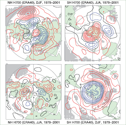
Figure 3.24. Linear trends in ERA-40 700 hPa geopotential height from 1979 to 2001 for DJF (top left and bottom right) and JJA (bottom left and top right), for the NH (left) and SH (right). Trends are contoured in 5 gpm per decade and are calculated from seasonal means of daily 1200 UTC fields. Red contours are positive, blue negative and black zero; the grey background indicates 1% statistical significance using a standard least squares F-test and assuming independence between years.
In the NH for 1979 to 2001 during DJF, increases in geopotential height occurred between 30°N and 50°N at many longitudes, notably over the central North Pacific( Figure 3.24 ). North of 60°N, height changes are consistent with recent occurrences of more neutral phases of the mean polar vortex. Increases in the 700 hPa height outweigh decreases in the northern summer (JJA) during 1979 to 2001 . At SH high latitudes, the largest changes are seen in the solstitial seasons( Figure 3.24 ), with changes of opposite sign in many areas between DJF and JJA. Changes during DJF reflect the increasing strength of the positive phase of the SAM (see Marshall, 2003 [JoC, SRC] ; Section 3.6.5 ), with large height decreases over Antarctica and corresponding height increases in the mid-latitudes, through the depth of the troposphere and into the stratosphere. The corresponding enhancement of the near-surface circumpolar westerlies at about 60°S, and associated changes in meridional winds in some sectors, is consistent with a warming trend observed at weather stations over the Antarctic Peninsula and Patagonia ( Thompson and Solomon, 2002 [PoC, JoC, ARC] ; see also Sections 3.2.2.4 and 3.6.5 ). In winter (JJA), there have been height increases over Antarctica since 1979, with a zonal wave 3 to wave 4 pattern of rises and falls in southern mid-latitudes. Trends up to 2001 are relatively strong and statistically significant, with annular modes in both hemispheres strongly positive during the 1990 s, although less so in recent years. Hence, geopotential height trends in DJF in the SH through 2004 have weakened in magnitude and significance, but with little change in spatial trend patterns.
Hemispheric teleconnections are strongly influenced by jet streams, which alter waves and storm tracks ( Branstator, 2002 [JoC] ). Using NRA from 1979 to 1995, Nakamura et al. 2002 [Ambiguous] ) found a weakening of the North Pacific winter jet since 1987, allowing efficient vertical coupling of upper-level disturbances with the surface temperature gradients ( Nakamura and Sampe, 2002 [JoC, SRC] ; Nakamura et al., 2004 [NPR, SRC] ). A trend from the 1970 s to the 1990 s towards a deeper polar vortex and Iceland Low associated with a positive phase of the NAM in winter ( Hurrell, 1995 [JoC, SRC] ; Thompson et al., 2000 [Ambiguous] ; Ostermeier and Wallace, 2003 [JoC] ) was accompanied by intensification and poleward displacement of the Atlantic polar frontal jet and associated enhancement of the Atlantic storm track activity ( Chang and Fu, 2002 [JoC, SRC] ; Harnik and Chang, 2003 [JoC, SRC] ). Analogous trends have also been found in the SH ( Gallego et al., 2005 [JoC] ).
3.5.3 Storm Tracks
Anumber of recent studies suggest that cyclone activity over both hemispheres has changed over the second half of the 20th century. General features include a poleward shift in storm track location, increased storm intensity, but a decrease in total storm numbers (e.g., Simmonds and Keay, 2000 [JoC, SRC] ; Gulev et al., 2001 [JoC, SRC] ; McCabe et al., 2001 [JoC] ). In the NH, McCabe et al. 2001 [JoC] ) found that there has been a significant decrease in mid-latitude cyclone activity and an increase in high-latitude cyclone frequency, suggesting a poleward shift of the storm track, with storm intensity increasing over the North Pacific and North Atlantic. In particular, Wang et al. 2006a [JoC, ARC] ) found that the North Atlantic storm track has shifted about 180 km northward in winter (JFM) during the past half century. The above findings are corroborated by Paciorek et al. 2002 [JoC] Simmonds and Keay 2002 [SRC] and Zhang et al. 2004b [JoC, ARC] ).
Several results suggest that cyclone activity in the NH mid-latitudes has increased during the past 40 years. Increases in storm track activity have been found in eddy statistics, based on NRA data. North Pacific storm track activity, identified as poleward eddy heat transport at 850 hPa, was significantly stronger during the late 1980 s and early 1990 s than during the early 1980 s ( Nakamura et al., 2002 [Ambiguous] ). A striking signal of decadal variability in Pacific storm track activity was its midwinter enhancement since 1987, despite a concurrent weakening of the Pacific jet, concomitant with the sudden weakening of the Siberian High ( Nakamura et al., 2002 [Ambiguous] ; Chang, 2003 [SRC] ). Significant increasing trends over both the Pacific and Atlantic are found in eddy meridional velocity variance at 300 hPa and other statistics ( Chang and Fu, 2002 [JoC, SRC] ; Paciorek et al., 2002 [JoC] ). Since 1980, there was an increase in the amount of eddy kinetic energy in the NH due to an increase in the efficiency in the conversion from potential to kinetic energy ( Hu et al., 2004 [JoC] Graham and Diaz 2001 [JoC] ) also found an increase in MSLP variance over the Pacific.
There are, however, significant uncertainties with such analyses, with some studies ( Bromirski et al., 2003 [JoC, SRC] ; Chang and Fu, 2003 [JoC, SRC] ) suggesting that storm track activity during the last part of the 20th century may not be more intense than the activity prior to the 1950 s. Eddy meridional velocity variance at 300 hPa in the NRA appears to be biased low prior to the mid- 1970 s, especially over east Asia and the western USA ( Harnik and Chang, 2003 [JoC, SRC] ). Hence, the increases in eddy variance in the NRA reanalysis data are nearly twice as large as that computed from rawinsonde observations. Better agreement is found for the Atlantic storm track exit region over Europe. Major differences between radiosonde and NRA temperature variance at 500 hPa over Asia ( Iskenderian and Rosen, 2000 [JoC] ; Paciorek et al., 2002 [JoC] ) also cast doubts on the magnitude of the increase in storm track activity, especially over the Pacific.
Station pressure data over the Atlantic-European sector (where records are long and consistent) show a decline of storminess from high levels during the late 19th century to a minimum around 1960 and then a quite rapid increase to a maximum around 1990, followed again by a slight decline ( Alexandersson et al., 2000 [SRC] ; Bärring and von Storch, 2004 [JoC] ; see also Section 3.8.4.1 ). However, changes in storm tracks are expected to be complex and depend on patterns of variability, and in practice, the noise present in the observations makes the detection of long-term changes in extratropical storm activity difficult. A more relevant approach seems to be the analysis of regional storminess in relation to spatial shifts and strength changes in teleconnection patterns (see Section 3.6 ).
Significant decreases in cyclone numbers, and increases in mean cyclone radius and depth over the southern extratropics over the last two or three decades ( Simmonds and Keay, 2000 [JoC, SRC] ; Keable et al., 2002 [JoC, SRC] ; Simmonds, 2003 [JoC, SRC] ; Simmonds et al., 2003 [JoC, SRC] ) have been associated with the observed trend in the SAM. Such changes, derived from NRA data, have been related to reductions in mid-latitude winter rainfall (e.g., the drying trend observed in south-western Australia ( Karoly, 2003 [Ambiguous] ) and to a circumpolar signal of increased precipitation off the coast of Antarctica ( Cai et al., 2003 [JoC, ARC] ). However, there are significant differences between ERA-40 and NRA in the SH: higher strong-cyclone activity and less weak-cyclone activity over all oceanic areas south of 40°S in all seasons, and stronger cyclone activity over the subtropics in the warm season in ERA-40, especially in the early decades ( Wang et al., 2006a [JoC, ARC] ).
3.5.4 Blocking
Blocking events, associated with persistent high-latitude ridging and a displacement of mid-latitude westerly winds lasting typically a week or two, are an important component of total circulation variability on intra-seasonal time scales. In the NH, the preferred locations for the blocking are over the Atlantic and the Pacific ( Tibaldi et al., 1994 [JoC, MoS] ), with a spring maximum and summer minimum in the Atlantic-European region ( Andrea et al., 1998 [JoC, MoS] ; Trigo et al., 2004 [PoC, JoC, ARC] ). Observations show that in the Euro-Atlantic sector, long-lasting (>10 day) blockings are clearly associated with the negative NAO phase ( Quadrelli et al., 2001 [JoC] ; Barriopedro et al., 2006 [JoC] ), whereas the blockings of 5 to 10 day duration exhibit no such relationship, pointing to the dynamical links between the life cycles of NAO and blocking events ( Scherrer et al, 2006 [JoC, ARC] ; Schwierz et al., 2006 [JoC] Wiedenmann et al. 2002 [JoC] ) did not find any long-term statistically significant trends in NH blocking intensity. However, in the Pacific sector, Barriopedro et al. 2006 [JoC] ) found a significant increase from 1948 to 2002 in western Pacific blocking days and events (57 and 62%, respectively). They also found less intense North Atlantic region blocking, with statistically significant decreases in events and days. Wiedenmann et al. 2002 [JoC] ) found that blocking events, especially in the North Pacific region, were significantly weaker during El Niño years.
In the SH, blocking occurrence is maximised over the southern Pacific ( Renwick and Revell, 1999 [JoC] ; Renwick, 2005 [JoC] ), with secondary blocking regions over the southern Atlantic and over the southern Indian Ocean and the Great Australian Bight. The frequency of blocking occurrence over the southeast Pacific is strongly ENSO-modulated ( Rutllant and Fuenzalida, 1991 [JoC] ; Renwick, 1998 [JoC] ), while in other regions, much of the interannual variability in occurrence appears to be internally generated ( Renwick, 2005 [JoC] ). A decreasing trend in blocking frequency and intensity for the SH as a whole from NRA ( Wiedenmann et al., 2002 [JoC] ) is consistent with observed increases in zonal winds across the southern oceans. However, an overall increasing trend in the frequency of long-lived positive height anomalies is evident in the reanalyses over the SH in the 1970 s ( Renwick, 2005 [JoC] ), apparently related to the introduction of satellite observations. Given data limitations, it may be too early to reliably define trends in SH blocking occurrence.
3.5.5 The Stratosphere
The dynamically stable stratospheric circulation is dominated in mid-latitudes by westerlies in the winter hemisphere and easterlies in the summer hemisphere, and the associated meridional overturning ‘Brewer-Dobson’ circulation. In the tropics, zonal winds reverse direction approximately every two years, in the downward-propagating QBO ( Andrews et al., 1987 [NPR] ). Ozone is formed predominantly in the tropics and transported to higher latitudes by the Brewer-Dobson circulation. Climatological stratospheric zonal-mean zonal winds (i.e., the westerly wind averaged over latitude circles) from different data sets show overall good agreement in the extratropics, whereas relatively large differences occur in the tropics ( Randel et al., 2004b [JoC] ).
The breaking of vertically propagating waves, originating from the troposphere, decelerates the stratospheric westerlies (see Box 3.3 ). This sometimes triggers ‘sudden warmings’ when the westerly polar vortex breaks down with an accompanying warming of the polar stratosphere, which can quickly reverse the latitudinal temperature gradient ( Kodera et al., 2000 [JoC] ). While no major warming occurred in the NH in nine consecutive winters during 1990 to 1998, seven major warmings occurred during 1999 to 2004 ( Manney et al., 2005 [JoC] ). As noted by Naujokat et al. 2002 [JoC] ), many of the recent stratospheric warmings after 2000 have been atypically early and the cold vortex recovered in March. In September 2002, a major warming was observed for the first time in the SH (e.g., Krüger et al., 2005 [JoC] ; Simmons et al., 2005 [JoC, MoS, SRC] ). This major warming followed a relatively weak winter polar vortex ( Newman and Nash, 2005 [NPR, JoC] ).
The analysis of past stratospheric changes relies on a combination of radiosonde information (available since the 1950 s), satellite information (available from the 1970 s) and global reanalyses. During the mid- 1990 s, the NH exhibited a number of years when the Arctic winter vortex was colder, stronger ( Kodera and Koide, 1997 [JoC] ; Pawson and Naujokat, 1999 [JoC] ) and more persistent ( Waugh et al., 1999 [JoC] ; Zhou et al., 2000 [JoC] ). Some analyses show a downward trend in the NH wave forcing in the period 1979 to 2000, particularly in January and February ( Newman and Nash, 2000 [JoC] ;( Randel et al., 2002 ) ). Trend calculations are, however, very sensitive to the month and period of calculation, so the detection of long-term change from a relatively short stratospheric data series is still problematic ( (Labitzke and Kunze, 2005 ) ).
In the SH, using radiosonde data, Thompson and Solomon 2002 [PoC, JoC, ARC] ) reported a significant decrease of the lower-stratospheric geopotential height averaged over the SH polar cap in October to March and May between 1969 and 1998 . The ERA-40 and NRA stratospheric height reanalyses indicate a trend towards a strengthening antarctic vortex since 1980 during summer (DJF; Renwick, 2004 [JoC] ; Section 3.5.2 ), largely related to ozone depletion ( Ramaswamy et al., 2001 [JoC, MoS, ARC] ; Gillett and Thompson, 2003 [JoC, MoS, ARC] ). The ozone hole has led to a cooling of the stratospheric polar vortex in late spring (October–November; Randel and Wu, 1999 [JoC] ), and to a two- to three-week delay in vortex breakdown ( Waugh et al., 1999 [JoC] ).
3.5.6 Winds, Waves and Surface Fluxes
Changes in atmospheric circulation imply associated changes in winds, wind waves and surface fluxes. Surface wind and meteorological observations from Voluntary Observing Ships (VOS) became systematic around 150 years ago and are assembled in ICOADS ( Worley et al., 2005 [JoC] ). Apparent significant trends in scalar wind should be considered with caution as VOS wind observations are influenced by time-dependent biases ( Gulev et al., 2007 [JoC, MoS, SRC, 2007] ), resulting from the rising proportion of anemometer measurements, increasing anemometer heights, changes in definitions of Beaufort wind estimates ( Cardone et al., 1990 [JoC] ), growing ship size, inappropriate evaluation of the true wind speed from the relative wind ( Gulev and Hasse, 1999 [JoC, SRC] ) and time-dependent sampling biases ( Sterl, 2001 [JoC] ; Gulev et al., 2007 [JoC, MoS, SRC, 2007] ). Consideration of time series of local surface pressure gradients ( Ward and Hoskins, 1996 [JoC, SRC] ) does not support the existence of any significant globally averaged trends in marine wind speeds, but reveals regional patterns of upward trends in the tropical North Atlantic and extratropical North Pacific and downward trends in the equatorial Atlantic, tropical South Atlantic and subtropical North Pacific (see also Sections 3.5.1 and 3.5.3 ).
Visual VOS observations of wind waves for more than a century, often measured as significant wave height (SWH, the highest one-third of wave (sea and swell) heights), have been less affected than marine winds by changes in observational practice, although they may suffer from time-dependent sampling uncertainty, which was somewhat higher at the beginning of the record. Local wind speed directly affects only the wind-sea component of SWH, while the swell component is largely influenced by the frequency and intensity of remote storms. Linear trends in the annual mean SWH from ship data ( Gulev and Grigorieva, 2004 [JoC, SRC] ) for 1900 to 2002 were significantly positive almost everywhere in the North Pacific, with a maximum upward trend of 8 to 10 cm per decade (up to 0.5% yr–1). These are supported by buoy records for 1978 to 1999 ( Allan and Komar, 2000 [JoC] ; Gower, 2002 [JoC] ) for annual and winter (October to March) mean SWH and confirmed by the long-term estimates of storminess derived from the tide gauge residuals ( Bromirski et al., 2003 [JoC, SRC] ) and hindcast data ( Graham and Diaz, 2001 [JoC] ), although Tuller 2004 [JoC] ) found primarily negative trends in wind off the west coast of Canada. In the Atlantic, centennial time series ( Gulev and Grigorieva, 2004 [JoC, SRC] ) show weak but statistically significant negative trends along the North Atlantic storm track, with a decrease of 5.2 cm per decade (0.25% yr–1)in the western Atlantic storm formation region. Regional model hindcasts (e.g., ( Vikebo et al., 2003; ) Weisse et al., 2005 [JoC, MoS] ) show growing SWH in the northern North Atlantic over the last 118 years.
Box 3.3: Stratospheric-Tropospheric Relations and Downward Propagation
The troposphere influences the stratosphere mainly through planetary-scale waves that propagate upward during the extended winter season when stratospheric winds are westerly. The stratosphere responds to this forcing from below to produce long-lived changes to the strength of the polar vortices. In turn, these fluctuations in the strength of the stratospheric polar vortices are observed to couple downward to surface climate ( Baldwin and Dunkerton, 1999 [JoC, SRC] , 2001; Kodera et al., 2000 [JoC] ; Limpasuvan et al., 2004 [JoC] ; Thompson et al., 2005 [Ambiguous] ). This relationship occurs in the zonal wind and can be seen clearly in annular modes, which explain a large fraction of the intra-seasonal and interannual variability in the troposphere ( Thompson and Wallace, 2000 [JoC] ) and most of the variability in the stratosphere ( Baldwin and Dunkerton, 1999 [JoC, SRC] ). Annular modes appear to arise naturally as a result of internal interactions within the troposphere and stratosphere ( Limpasuvan and Hartmann, 2000 [JoC] ; Lorenz and Hartmann, 2001 [JoC] , 2003 ).
The relationship between NAM anomalies in the stratosphere and troposphere can be seen in Box 3.3 ,Figure 1, in which the NAM index at 10 hPa is used to define events when the stratospheric polar vortex was extremely weak (stratospheric warmings). On average, weak vortex conditions in the stratosphere tend to descend to the troposphere and are followed by negative NAM anomalies at the surface for more than two months. Anomalously strong vortex conditions propagate downwards in a similar way.
Long-lived annular mode anomalies in the lowermost stratosphere appear to lengthen the time scale of the surface NAM. The tropospheric annular mode time scale is longest during winter in the NH, but longest during late spring (November–December) in the SH ( Baldwin et al., 2003 [JoC, MoS, SRC] ). In both hemispheres, the time scale of the tropospheric annular modes is longest when the variance of the annular modes is greatest in the lower stratosphere.
Downward coupling to the surface depends on having large circulation anomalies in the lowermost stratosphere. In such cases, the stratosphere can be used as a statistical predictor of the monthly mean surface NAM on time scales of up to two months ( Baldwin et al., 2003 [JoC, MoS, SRC] ; Scaife et al., 2005 [JoC] ). Similarly, SH trends in temperature and geopotential height, associated with the ozone hole, appear to couple downward to affect high-latitude surface climate ( Thompson and Solomon, 2002 [PoC, JoC, ARC] ; Gillett and Thompson, 2003 [JoC, MoS, ARC] ). As the stratospheric circulation changes with ozone depletion or increasing greenhouse gases, those changes will likely be reflected in changes to surface climate. Thompson and Solomon 2005 [PoC, JoC, ARC] ) showed that the spring strengthening and cooling of the SH polar stratospheric vortex preceded similarly signed trends in the SH tropospheric circulation by one month in the interval 1973 to 2003 . They argued that similar downward coupling is not evident in the NH geopotential trends computed using monthly radiosonde data. An explanation for this difference may be that the stratospheric signal is stronger in the SH, mainly due to ozone depletion, giving a more robust downward coupling.
The dynamical mechanisms by which the stratosphere influences the troposphere are not well understood, but the relatively large surface signal implies that the stratospheric signal is amplified. The processes likely involve planetary waves ( Song and Robinson, 2004 [JoC, ARC] ) and synoptic-scale waves ( Wittman et al., 2004 [JoC] ), which interact with stratospheric zonal wind anomalies near the tropopause. The altered waves would be expected to affect tropospheric circulation and induce surface pressure changes corresponding to the annular modes ( Wittman et al., 2004 [JoC] ).
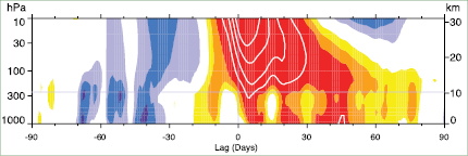
Box 3.3 ,Figure 1. Composites of time-height development of the NAM index for 18 weak vortex events. The events are selected by the dates on which the 10 hPa annular mode index crossed –3.0. Day 0 is the start of the weak vortex event. The indices are non-dimensional; the contour interval for the colour shading is 0.25, and 0.5 for the white lines. Values between –0.25 and 0.25 are not shaded. Yellow and red shading indicates negative NAM indices and blue shading indicates positive indices. The thin horizontal lines indicate the approximate boundary between the troposphere and the stratosphere. Modified from Baldwin and Dunkerton 2001 [JoC, SRC] ).
Linear trends in SWH for the period 1950 to 2002 ( Figure 3.25 )are statistically significant and positive over most of the mid-latitudinal North Atlantic and North Pacific, as well as in the western subtropical South Atlantic, the eastern equatorial Indian Ocean and the East China and South China Seas. The largest upward trends (14 cm per decade) occur in the northwest Atlantic and the northeast Pacific. Statistically significant negative trends are observed in the western Pacific tropics, the Tasman Sea and the south Indian Ocean (–11 cm per decade).
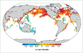
Figure 3.25. Estimates of linear trends in significant wave height (cm per decade) for regions along the major ship routes of the global ocean for 1950 to 2002 . Trends are shown only for locations where they are significant at the 5% level. Adapted from Gulev and Grigorieva 2004 [JoC, SRC] ).
Hindcasts of waves with global and basin-scale models by Wang and Swail 2001 [JoC] , 2002 and Sterl and Caires 2005 [JoC] ), based on NRA and ERA-40 winds, respectively, show an increasing mean SWH as well as intensification of SWH extremes during the last 40 years, with the 99% extreme of the winter SWH increasing in the northeast Atlantic by a maximum of 0.4 m per decade. Wave height hindcasts driven with NRA surface winds suggest that worsening wave conditions in the northeastern North Atlantic during the latter half of the 20th century were connected to a northward displacement in the storm track, with decreasing wave heights in the southern North Atlantic ( (Lozano and Swail, 2002 ) ). Increases of SWH in the North Atlantic mid-latitudes are further supported by a 14-year ( 1988 – 2002 ) time series of the merged TOPography EXperiment (TOPEX)/Poseidon and European Remote Sensing (ERS-1/2) satellite altimeter data ( Woolf et al., 2002 [JoC, MoS] ).
Since the TAR, research into surface fluxes has continued to be directed at improving the accuracy of the mean air-sea exchange fields (particularly of heat) with less work on long-term trends. Significant uncertainties remain in global fields of the net heat exchange, stemming from problems in obtaining accurate estimates of the different heat flux components. Estimates of surface flux variability from reanalyses are strongly influenced by inhomogeneous data assimilation input, especially in the Southern Ocean, and Sterl 2004 [JoC] ) reported that variability of the surface latent heat flux in the Southern Ocean became much more reliable after 1979, when observations increased. Recent evaluations of heat flux estimates from reanalyses and in situ observations indicate some improvements but there are still global biases of several tens of watts per square metre in unconstrained products based on VOS observations ( Grist and Josey, 2003 [JoC, SRC] ). Estimates of the implied ocean heat transport from the NRA, indirect residual techniques and some coupled models are in reasonable agreement with hydrographic observations ( Trenberth and Caron, 2001 [PoC, JoC, MoS, SRC] ; Grist and Josey, 2003 [JoC, SRC] ). However, the hydrographic observations also contain significant uncertainties (see Chapter5 )due to both interannual variability and assumptions made in the computation of the heat transport, and these must be recognised when using them to evaluate the various flux products. For the North Atlantic, there are indications of positive trends in the net heat flux from the ocean of 10 Wm–2 per decade in the western subpolar gyre and coherent negative changes in the eastern subtropical gyre, closely correlated with the NAO variability in the interval 1948 to 2002 ( Marshall et al., 2001 [JoC] ; Visbeck et al., 2003 [NPR] ; Gulev et al., 2007 [JoC, MoS, SRC, 2007] ).
3.5.7 Summary
Changes from the late 1970 s to recent years generally reveal decreases in tropospheric geopotential heights over high latitudes of both hemispheres and increases over the mid-latitudes in DJF. The changes amplify with altitude up to the lower stratosphere, but remain similar in shape to lower atmospheric levels and are associated with the intensification and poleward displacement of corresponding Atlantic and southern polar front jet streams and enhanced storm track activity. Based on a variety of measurements at the surface and in the upper troposphere, it is likely that there has been an increase and a poleward shift in NH winter storm-track activity over the second half of the 20th century, but there are still significant uncertainties in the magnitude of the increase due to time-dependent biases in the reanalyses. Analysed decreases in cyclone numbers over the southern extratropics and increases in mean cyclone radius and depth over much of the SH over the last two decades are subject to even larger uncertainties.
The decrease in long-lasting blocking frequency over the North Atlantic-European sector over recent decades is dynamically consistent with NAO variability (see Section 3.6 ), but given data limitations, it may be too early to define the nature of any trends in SH blocking occurrence, despite observed trends in the SAM. After the late 1990 s in the NH, occurrences of major sudden warmings seem to have increased in the polar stratosphere, associated with the occurrence of more neutral states of the tropospheric and stratospheric vortex. In the SH, there has been a strengthening tropospheric antarctic vortex during summer in association with the ozone hole, which has led to a cooling of the stratospheric polar vortex in late spring and to a two- to three-week delay in vortex breakdown. In September 2002, a major warming was observed for the first and only time in the SH. Analysis of observed wind and SWH support the reanalysis-based evidence for an increase in storm activity in the extratropical NH in recent decades (see also Section 3.6 )until the late 1990 s. For heat flux, there seem to have been NAO-related variations over the Labrador Sea, which is a key region for deep water formation.
3.6 Patterns of Atmospheric Circulation Variability
3.6.1 Teleconnections
The global atmospheric circulation has a number of preferred patterns of variability, all of which have expressions in surface climate. Box 3.4 discusses the main patterns and associated indices. Regional climates in different locations may vary out of phase, owing to the action of such ‘teleconnections’, which modulate the location and strength of the storm tracks( Section 3.5.3 )and poleward fluxes of heat, moisture and momentum. A comprehensive review by Hurrell et al. 2003 [NPR, SRC] ) has been updated by new analyses, notably from Quadrelli and Wallace 2004 [JoC] and Trenberth et al. 2005b [PoC, JoC, SRC] ). Understanding the nature of teleconnections and changes in their behaviour is central to understanding regional climate variability and change. Such seasonal and longer time-scale anomalies have direct impacts on humans, as they are often associated with droughts, floods, heat waves and cold waves and other changes that can severely disrupt agriculture, water supply and fisheries, and can modulate air quality, fire risk, energy demand and supply and human health.
The analysis of teleconnections has typically employed a linear perspective, which assumes a basic spatial pattern with varying amplitude and mirror image positive and negative polarities ( Hurrell et al., 2003 [NPR, SRC] ; Quadrelli and Wallace, 2004 [JoC] ). In contrast, nonlinear interpretations would identify preferred climate anomalies as recurrent states of a specific polarity (e.g., Corti et al., 1999 [JoC, ARC] ; Cassou and Terray, 2001 [JoC, SRC] ; Monahan et al., 2001 [JoC, ARC] ). Climate change may result through changes from one quasi-stationary state to another, as a preference for one polarity of a pattern ( Palmer, 1999 [JoC, MoS, ARC] ), or through a change in the nature or number of states ( Straus and Molteni, 2004 [JoC, MoS] ).
In the NH, one-point correlation maps illustrate the Pacific-North American (PNA) pattern and the NAO( Figure 3.26 ), but in the SH, wave structures do not emerge as readily owing to the dominance of the SAM. Although teleconnections are best defined over a grid, simple indices based on a few key station locations remain attractive as the series can often be carried back in time long before complete gridded fields were available (see Section 3.6.4 , Figure 3.31 ); the disadvantage is increased noise from the reduced spatial sampling. For instance, Hurrell et al. 2003 [NPR, SRC] ) found that the residence time of the NAO in its positive phase in the early 20th century was not as great as indicated by the positive NAO index for that period.
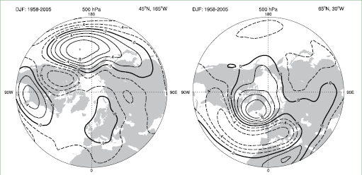
Figure 3.26. The PNA (left) and NAO (right) teleconnection patterns, shown as one-point correlation maps of 500 hPa geopotential heights for boreal winter (DJF) over 1958 to 2005 . In the left panel, the reference point is 45°N, 165°W, corresponding to the primary centre of action of the PNA pattern, given by the + sign. In the right panel, the NAO pattern is illustrated based on a reference point of 65°N, 30°W. Negative correlation coefficients are dashed, and the contour increment is 0.2. Adapted from Hurrell et al. 2003 [NPR, SRC] ).
Many teleconnections have been identified, but combinations of only a small number of patterns can account for much of the interannual variability in the circulation and surface climate. Quadrelli and Wallace 2004 [JoC] ) found that many patterns of NH interannual variability can be reconstructed as linear combinations of the first two Empirical Orthogonal Functions (EOFs) of sea level pressure (approximately the NAM and the PNA). Trenberth et al. 2005b [PoC, JoC, SRC] ) analysed global atmospheric mass and found four key rotated EOF patterns: the two annular modes (SAM and NAM), a global ENSO-related pattern and a fourth closely related to the North Pacific Index and the PDO, which in turn is closely related to ENSO and the PNA pattern.
Teleconnection patterns tend to be most prominent in the winter (especially in the NH), when the mean circulation is strongest. The strength of teleconnections and the way they influence surface climate also vary over long time scales. Both the NAO and ENSO exhibited marked changes in their surface climate expressions on multi-decadal time scales during the 20th century (e.g., Power et al., 1999b [JoC, ARC] ; Jones et al., 2003 [Ambiguous] ). Multi-decadal changes in influence are often real and not due just to poorer data quality in earlier decades.
Box 3.4: Defining the Circulation Indices
Ateleconnection is made up of a fixed spatial pattern with an associated index time series showing the evolution of its amplitude and phase. Teleconnections are best defined by values over a grid but it is often convenient to devise simplified indices based on key station values. A classic example is the Southern Oscillation (SO), encompassing the entire tropical Pacific, yet encapsulated by a simple SO Index (SOI), based on differences between Tahiti (eastern Pacific) and Darwin (western Pacific) MSLP anomalies.
Anumber of teleconnections have historically been defined from either station data (SOI, NAO) or from gridded fields (NAM, SAM, PDO/NPI and PNA):
- Southern Oscillation Index (SOI). The MSLP anomaly difference of Tahiti minus Darwin, normalised by the long-term mean and standard deviation of the MSLP difference (Troup, 1965; Können et al., 1998). Available from the 1860s. Darwin can be used alone, as its data are more consistent than Tahiti prior to 1935.
- North Atlantic Oscillation (NAO) Index. The difference of normalised MSLP anomalies between Lisbon, Portugal and Stykkisholmur, Iceland has become the most widely used NAO index and extends back in time to 1864 (Hurrell, 1995), and to 1821 if Reykjavik is used instead of Stykkisholmur and Gibraltar instead of Lisbon (Jones et al., 1997).
- Northern Annular Mode (NAM) Index. The amplitude of the pattern defined by the leading empirical orthogonal function of winter monthly mean NH MSLP anomalies poleward of 20°N (Thompson and Wallace, 1998, 2000). The NAM has also been known as the Arctic Oscillation (AO), and is closely related to the NAO.
- Southern Annular Mode (SAM) Index. The difference in average MSLP between SH middle and high latitudes (usually 45°S and 65°S), from gridded or station data (Gong and Wang, 1999; Marshall, 2003), or the amplitude of the leading empirical orthogonal function of monthly mean SH 850 hPa height poleward of 20°S (Thompson and Wallace, 2000). Formerly known as the Antarctic Oscillation (AAO) or High Latitude Mode (HLM).
- Pacific-North American pattern (PNA) Index. The mean of normalised 500 hPa height anomalies at 20°N, 160°W and 55°N, 115°W minus those at 45°N, 165°W and 30°N, 85°W (Wallace and Gutzler, 1981).
- Pacific Decadal Oscillation (PDO) Index and North Pacific Index (NPI). The NPI is the average MSLP anomaly in the Aleutian Low over the Gulf of Alaska (30°N–65°N, 160°E–140°W; Trenberth and Hurrell, 1994) and is an index of the PDO, which is also defined as the pattern and time series of the first empirical orthogonal function of SST over the North Pacific north of 20°N (Mantua et al., 1997; Deser et al., 2004). The PDO broadened to cover the whole Pacific Basin is known as the Inter-decadal Pacific Oscillation (IPO: Power et al., 1999b). The PDO and IPO exhibit virtually identical temporal evolution (Folland et al., 2002).
3.6.2 El Niño-Southern Oscillation and Tropical/Extratropical Interactions
3.6.2.1 El Niño-Southern Oscillation
El Niño-Southern Oscillation events are a coupled ocean-atmosphere phenomenon. El Niño involves warming of tropical Pacific surface waters from near the International Date Line to the west coast of South America, weakening the usually strong SST gradient across the equatorial Pacific, with associated changes in ocean circulation. Its closely linked atmospheric counterpart, the Southern Oscillation (SO), involves changes in trade winds, tropical circulation and precipitation. Historically, El Niño events occur about every 3 to 7 years and alternate with the opposite phases of below-average temperatures in the eastern tropical Pacific (La Niña). Changes in the trade winds, atmospheric circulation, precipitation and associated atmospheric heating set up extratropical responses. Wavelike extratropical teleconnections are accompanied by changes in the jet streams and storm tracks in mid-latitudes ( Chang and Fu, 2002 [JoC, SRC] ).
The El Niño-Southern Oscillation has global impacts, manifested most strongly in the northern winter months (November–March). Anomalies in MSLP are much greater in the extratropics while the tropics feature large precipitation variations. Associated patterns of surface temperature and precipitation anomalies around the globe are given in Figure 3.27 ( Trenberth and Caron, 2000 [PoC, JoC, SRC] ), and the evolution of these patterns and links to global mean temperature perturbations are given by Trenberth et al. 2002b [PoC, JoC, SRC] ).
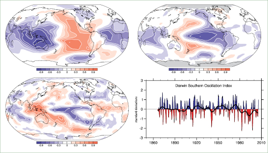
Figure 3.27. Correlations with the SOI, based on normalised Tahiti minus Darwin sea level pressures, for annual (May to April) means for sea level pressure (top left) and surface temperature (top right) for 1958 to 2004, and GPCP precipitation for 1979 to 2003 (bottom left), updated from Trenberth and Caron 2000 [PoC, JoC, SRC] ). The Darwin-based SOI, in normalized units of standard deviation, from 1866 to 2005 ( Können et al., 1998 [JoC] ; lower right) features monthly values with an 11-point low-pass filter, which effectively removes fluctuations with periods of less than eight months ( Trenberth, 1984 [PoC, JoC, SRC] ). The smooth black curve shows decadal variations (see Appendix 3.A ). Red values indicate positive sea level pressure anomalies at Darwin and thus El Niño conditions.
The nature of ENSO has varied considerably over time. Strong ENSO events occurred from the late 19th century through the first 25 years of the 20th century and again after about 1950, but there were few events of note from 1925 to 1950 with the exception of the major 1939 – 1941 event( Figure 3.27 ). The 1976 – 1977 climate shift ( Trenberth, 1990 [PoC, JoC, SRC] ; see Figure 3.27 and Section 3.6.3 , Figure 3.28 )was associated with marked changes in El Niño evolution ( Trenberth and Stepaniak, 2001 [PoC, JoC, SRC] ), a shift to generally above-normal SSTs in the eastern and central equatorial Pacific and a tendency towards more prolonged and stronger El Niños. Since the TAR, there has been considerable work on decadal and longer-term variability of ENSO and Pacific climate. Such decadal atmospheric and oceanic variations( Section 3.6.3 )are more pronounced in the North Pacific and across North America than in the tropics but are also present in the South Pacific, with evidence suggesting they are at least in part forced from the tropics ( Deser et al., 2004 [JoC, SRC] ).
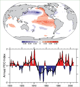
Figure 3.28. Pacific Decadal Oscillation: (top) SST based on the leading EOF SST pattern for the Pacific basin north of 20°N for 1901 to 2004 (updated; see Mantua et al., 1997 [JoC] ; Power et al., 1999b [JoC, ARC] ) and projected for the global ocean (units are nondimensional); and (bottom) annual time series (updated from Mantua et al., 1997 [JoC] ). The smooth black curve shows decadal variations (see Appendix 3.A ).
El Niño-Southern Oscillation events involve large exchanges of heat between the ocean and atmosphere and affect global mean temperatures. The 1997 – 1998 event was the largest on record in terms of SST anomalies and the global mean temperature in 1998 was the highest on record (at least until 2005 Trenberth et al. 2002b [PoC, JoC, SRC] ) estimated that global mean surface air temperatures were 0.17°C higher for the year centred on March 1998 owing to the El Niño. Extremes of the hydrological cycle such as floods and droughts are common with ENSO and are apt to be enhanced with global warming ( Trenberth et al., 2003 [PoC, JoC, SRC] ). For example, the modest 2002 – 2003 El Niño was associated with a drought in Australia, made much worse by record-breaking heat ( Nicholls, 2004 [JoC, SRC] ; and see Section 3.8.4 , Box 3.6 ). Thus, whether observed changes in ENSO behaviour are physically linked to global climate change is a research question of great importance.
3.6.2.2 Tropical-Extratropical Teleconnections: PNA and PSA
Circulation variability over the extratropical Pacific features wave-like patterns emanating from the subtropical western Pacific, characteristic of Rossby wave propagation associated with anomalous tropical heating ( Horel and Wallace, 1981 [JoC] ; Hoskins and Karoly, 1981 [JoC, MoS, SRC] ). These are known as the PNA and Pacific-South American (PSA) patterns and can arise naturally through atmospheric dynamics as well as in response to heating. Over the NH in winter, the PNA pattern lies across North America from the subtropical Pacific, with four centres of action( Figure 3.26 ). While the PNA pattern can be illustrated by taking a single point correlation, this is not so easy for the PSA pattern (not shown), as its spatial centres of action are not fixed. However, the PSA pattern can be present at all times of year, lying from Australasia over the southern Pacific and Atlantic ( Mo and Higgins, 1998 [JoC] ; Kidson, 1999 [JoC] ; Mo, 2000 [JoC] ).
The PNA, or a variant of it ( Straus and Shukla, 2002 [JoC, ARC] ), is associated with modulation of the Aleutian Low, the Asian jet, and the Pacific storm track, affecting precipitation in western North America and the frequency of Alaskan blocking events and associated cold air outbreaks over the western USA in winter ( Compo and Sardeshmukh, 2004 [JoC, MoS] ). The PSA is associated with modulation of the westerlies over the South Pacific, effects of which include significant rainfall variations over New Zealand, changes in the nature and frequency of blocking events across the high-latitude South Pacific, and interannual variations in antarctic sea ice across the Pacific and Atlantic sectors ( Renwick and Revell, 1999 [JoC] ; Kwok and Comiso, 2002a [JoC, ARC] ; Renwick, 2002 [JoC] ). While both PNA and PSA activity have varied with decadal modulation of ENSO, no systematic changes in their behaviour have been reported.
3.6.3 Pacific Decadal Variability
Decadal to inter-decadal variability of the atmospheric circulation is most prominent in the North Pacific, where fluctuations in the strength of the winter Aleutian Low pressure system co-vary with North Pacific SST in the PDO. These are linked to decadal variations in atmospheric circulation, SST and ocean circulation throughout the whole Pacific Basin in the Inter-decadal Pacific Oscillation (IPO; Trenberth and Hurrell, 1994 [PoC, JoC, SRC] ; Gershunov and Barnett, 1998 [JoC] ; Folland et al., 2002 [PoC, JoC, SRC] ; McPhaden and Zhang, 2002 [JoC, ARC] ; Deser et al., 2004 [JoC, SRC] ). Key measures of Pacific decadal variability are the North Pacific Index (NPI; Trenberth and Hurrell, 1994 [PoC, JoC, SRC] ), PDO index ( Mantua et al., 1997 [JoC] ) and the IPO index ( Power et al., 1999b [JoC, ARC] ; Folland et al., 2002 [PoC, JoC, SRC] ; see Figures 3.28 and 3.29 ). Modulation of ENSO by the PDO significantly modifies regional teleconnections around the Pacific Basin ( Power et al., 1999b [JoC, ARC] ; Salinger et al., 2001 [JoC, ARC] ), and affects the evolution of the global mean climate.
The PDO/IPO has been described as a long-lived El Niño-like pattern of Indo-Pacific climate variability ( Knutson and Manabe, 1998 [JoC, MoS, ARC] ; Evans et al., 2001 [JoC] ; Deser et al., 2004 [JoC, SRC] ; Linsley et al., 2004 [JoC] ) or as a low-frequency residual of ENSO variability on multi-decadal time scales ( Newman et al., 2003 [JoC] ). Indeed, the symmetry of the SST anomaly pattern between the NH and SH may be a reflection of common tropical forcing. However, Folland et al. 2002 [PoC, JoC, SRC] ) showed that the IPO significantly affects the movement of the South Pacific Convergence Zone in a way independent of ENSO (see also Deser et al., 2004 [JoC, SRC] ). Other results indicate that the extratropical phenomena are generic components of the PDO ( Deser et al., 1996 [JoC, SRC] , 1999, 2003; Gu and Philander, 1997 [JoC] ). The extratropics may also contribute to the tropical SST changes via an ‘atmospheric bridge’, confounding the simple interpretation of a tropical origin ( Barnett et al., 1999 [JoC] ; Vimont et al., 2001 [JoC] ).
The inter-decadal time scale of tropical Indo-Pacific SST variability is likely due to oceanic processes. Extratropical ocean influences are also likely to play a role as changes in the ocean gyre evolve and heat anomalies are subducted and re-emerge ( Deser et al., 1996 [JoC, SRC] , 1999, 2003; Gu and Philander, 1997 [JoC] ). It is also possible that there is no well-defined coupled ocean-atmosphere ‘mode’ of variability in the Pacific on decadal to inter-decadal time scales, since instrumental records are too short to provide a robust assessment and palaeoclimate records conflict regarding time scales ( Biondi et al., 2001 [JoC, SRC] ; Gedalof et al., 2002 [JoC] Schneider and Cornuelle 2005 [JoC, MoS] ) suggested that the PDO is not itself a mode of variability but is a blend of three phenomena. They showed that the observed PDO pattern and evolution can be recovered from a reconstruction of North Pacific SST anomalies based on a first order autoregressive model and forcing by variability of the Aleutian low, ENSO and oceanic zonal advection in the Kuroshio-Oyashio Extension. The latter results from oceanic Rossby waves that are forced by North Pacific Ekman pumping. The SST response patterns to these processes are not completely independent, but they determine the spatial characteristics of the PDO. Under this hypothesis, the key physical variables for measuring Pacific climate variability are ENSO and NPI (Aleutian Low) indices, rather than the PDO index.
Figure 3.29 (top) shows a time series of the NPI for 1900 to 2005 ( Deser et al., 2004 [JoC, SRC] ). There is substantial low-frequency variability, with extended periods of predominantly high values indicative of a weakened circulation ( 1900 – 1924 and 1947 – 1976 ) and predominantly low values indicative of a strengthened circulation ( 1925 – 1946 and 1977 – 2005 ). The well-known decrease in pressure from 1976 to 1977 is analogous to transitions that occurred from 1946 to 1947 and from 1924 to 1925, and these earlier changes were also associated with SST fluctuations in the tropical Indian( Figure 3.29 ,lower) and Pacific Oceans although not in the upwelling zone of the equatorial eastern Pacific ( Minobe, 1997 [JoC] ; Deser et al., 2004 [JoC, SRC] ). In addition, the NPI exhibits variability on shorter time scales, interpreted in part as a bi-decadal rhythm ( Minobe, 1999 [JoC] ).
Figure 3.29. (Top) Time series of the NPI (sea level pressure during December through March averaged over the North Pacific, 30°N to 65°N, 160°E to 140°W) from 1900 to 2005 expressed as normalised departures from the long-term mean (each tick mark on the ordinate represents two standard deviations, or 5.5 hPa). This record reflects the strength of the winter Aleutian Low pressure system, with positive (negative) values indicative of a weak (strong) Aleutian Low. The bars give the winter series and the smooth black curves show decadal variations (see Appendix 3.A ). Values were updated and extended to earlier decades from Trenberth and Hurrell 1994 [PoC, JoC, SRC] ). (Bottom) As above but for SSTs averaged over the tropical Indian Ocean (10°S–20°N, 50°E –125°E; each tick mark represents two standard deviations, or 0.36°C). This record has been inverted to facilitate comparison with the top panel. The dashed vertical lines mark years of transition in the Aleutian Low record ( 1925, 1947, 1977 ). Updated from Deser et al. 2004 [JoC, SRC] ).
There is observational and modelling evidence ( Pierce, 2001 [ARC] ; Schneider and Cornuelle, 2005 [JoC, MoS] ) suggesting the PDO/IPO does not excite the climate shifts in the Pacific area, but they share the same forcing. The 1976 – 1977 climate shift in the Pacific, associated with a phase change in the PDO from negative to positive, was associated with significant changes in ENSO evolution ( Trenberth and Stepaniak, 2001 [PoC, JoC, SRC] ) and with changes in ENSO teleconnections and links to precipitation and surface temperatures over North and South America, Asia and Australia ( Trenberth, 1990 [PoC, JoC, SRC] ; Trenberth and Hurrell, 1994 [PoC, JoC, SRC] ; Power et al., 1999a [JoC, ARC] ; Salinger et al., 2001 [JoC, ARC] ;( Mantua and Hare, 2002; ) Minobe and Nakanowatari, 2002 [JoC] ; Trenberth et al., 2002b [PoC, JoC, SRC] ; Deser et al., 2004 [JoC, SRC] ; Marengo, 2004 [Ambiguous] Schneider and Cornuelle 2005 [JoC, MoS] ) added extra credence to the hypothesis that the 1976 – 1977 climate shift is of tropical origin.
3.6.4 The North Atlantic Oscillation and Northern Annular Mode
The only teleconnection pattern prominent throughout the year in the NH is the NAO ( Barnston and Livezey, 1987 [JoC] ). It is primarily a north-south dipole in sea level pressure characterised by simultaneous out-of-phase pressure and height anomalies between temperate and high latitudes over the Atlantic sector, and therefore corresponds to changes in the westerlies across the North Atlantic into Europe( Figure 3.30 ). The NAO has the strongest signature in the winter months (December to March) when its positive (negative) phase exhibits an enhanced (diminished) Iceland Low and Azores High ( Hurrell et al., 2003 [NPR, SRC] ). The NAO is the dominant pattern of near-surface atmospheric circulation variability over the North Atlantic, accounting for one third of the total variance in monthly MSLP in winter. It is closely related to the NAM, which has similar structure over the Atlantic but is more zonally symmetric. The leading winter pattern of variability in the lower stratosphere is also annular, but the MSLP anomaly pattern that is associated with it is confined almost entirely to the Arctic and Atlantic sectors and coincides with the spatial structure of the NAO ( Deser, 2000 [JoC, SRC] ; see also Section 3.5.5 and Box 3.3 ).
Figure 3.30. Changes in winter (December–March) surface pressure, temperature, and precipitation corresponding to a unit deviation of the NAO index over 1900 to 2005 . (Top left) Mean sea level pressure (0.1 hPa). Values greater than 0.5 hPa are stippled and values less than −0.5 hPa are hatched. (Top right) Land-surface air and sea surface temperatures (0.1°C; contour increment 0.2°C). Temperature changes greater than 0.1°C are indicated by stippling, those less than –0.1°C are indicated by hatching, and regions of insufficient data (e.g., over much of the Arctic) are not contoured. (Bottom left) Precipitation for 1979 to 2003 based on GPCP (0.1 mm per day; contour interval 0.6 mm per day). Stippling indicates values greater than 0.3 mm per day and hatching values less than –0.3 mm per day. Adapted and updated from Hurrell et al. 2003 [NPR, SRC] ).
There is considerable debate over whether the NAO or the NAM is more physically relevant to the winter circulation ( Deser, 2000 [JoC, SRC] ; Ambaum et al., 2001 [JoC, SRC] , 2002 ), but the time series are highly correlated in winter( Figure 3.31 ). As Quadrelli and Wallace 2004 [JoC] ) showed, they are near neighbours in terms of their spatial patterns and their temporal evolution. The annular modes are intimately linked to the configuration of the extratropical storm tracks and jet streams. Changes in the phase of the annular modes appear to occur as a result of interactions between the eddies and the mean flow, and external forcing is not required to sustain them ( De Weaver and Nigam, 2000 [JoC] ). In the NH, stationary waves provide most of the eddy momentum fluxes, although transient eddies are also important. To the extent that the intrinsic excitation of the NAO/NAM pattern is limited to a period less than a few days ( Feldstein, 2002 [JoC] ), it should not exhibit year-to-year autocorrelation in conditions of constant forcing. Proxy and instrumental data, however, show evidence for intervals with prolonged positive and negative NAO index values in the last few centuries ( Cook et al., 2002 [PoC, JoC, ARC] ; Jones et al., 2003 [Ambiguous] ). In winter, a reversal occurred from the minimum index values in the late 1960 s to strongly positive NAO index values in the mid- 1990 s. Since then, NAO values have declined to near the long-term mean( Figure 3.31 ). In summer, Hurrell et al. 2001 [NPR, PoC, SRC] , 2002 ) identified significant interannual to multi-decadal fluctuations in the NAO pattern, and the trend towards persistent anticyclonic flow over northern Europe has contributed to anomalously warm and dry conditions in recent decades ( Rodwell, 2003 [NPR, MoS] ).
Figure 3.31. Normalised indices (units of standard deviation) of the mean winter (December–March) NAO developed from sea level pressure data. In the top panel, the index is based on the difference of normalised sea level pressure between Lisbon, Portugal and Stykkisholmur/Reykjavik, Iceland from 1864 to 2005 . The average winter sea level pressure data at each station were normalised by dividing each seasonal pressure anomaly by the long-term ( 1864 to 1983 ) standard deviation. In the middle panel, the index is the principal component time series of the leading EOF of Atlantic-sector sea level pressure. In the lower panel, the index is the principal component time series of the leading EOF of NH sea level pressure. The smooth black curves show decadal variations (see Appendix 3.A ). The individual bar corresponds to the January of the winter season (e.g., 1990 is the winter of 1989 / 1990 ). Updated from Hurrell et al. 2003 [NPR, SRC] ); see http://www.cgd.ucar.edu/cas/jhurrell/indices.html for updated time series.
Feldstein 2002 [JoC] ) suggested that the trend and increase in the variance of the NAO/NAM index from 1968 through 1997 was greater than would be expected from internal variability alone, while NAO behaviour during the first 60 years of the 20th century was consistent with atmospheric internal variability. However, the results are not so clear if based on just the period 1975 to 2004 ( Overland and Wang, 2005 [JoC, ARC] ). Although monthly-scale NAO variability is strong ( Czaja et al., 2003 [NPR] ; Thompson et al., 2003 [NPR, SRC] ), there may be predictability from stratospheric influences ( Thompson et al., 2002 [Ambiguous] ; Scaife et al., 2005 [JoC] ; see Box 3.3 ). There is mounting evidence that the recent observed inter-decadal NAO variability comes from tropical and extratropical ocean influences ( Hurrell et al., 2003 [NPR, SRC] , 2004 ), land surface forcing ( Gong et al., 2003 [JoC, MoS] ; Bojariu and Gimeno, 2003 [JoC] ) and from other external factors ( Gillett et al., 2003 [JoC, ARC] ).
The NAO exerts a dominant influence on winter surface temperatures across much of the NH( Figure 3.30 ), and on storminess and precipitation over Europe and North Africa. When the NAO index is positive, enhanced westerly flow across the North Atlantic in winter moves warm moist maritime air over much of Europe and far downstream, with dry conditions over southern Europe and northern Africa and wet conditions in northern Europe, while stronger northerly winds over Greenland and northeastern Canada carry cold air southward and decrease land temperatures and SST over the northwest Atlantic. Temperature variations over North Africa and the Middle East (cooling) and the southeastern USA (warming), associated with the stronger clockwise flow around the subtropical Atlantic high-pressure centre, are also notable. Following on from Hurrell 1996 [JoC, SRC] Thompson et al. 2000 [Ambiguous] ) showed that for JFM from 1968 to 1997, the NAM accounted for 1.6°C of the 3.0°C warming in Eurasian surface temperatures, 4.9 hPa of the 5.7 hPa decrease in sea level pressure from 60°N to 90°N; 37% out of the 45% increase in Norwegian-area precipitation (55°N–65°N, 5°E–10°E), and 33% out of the 49% decrease in Spanish-region rainfall (35°N–45°N, 10°W–0°W). There were also significant effects on ocean heat content, sea ice, ocean currents and ocean heat transport.
Positive NAO index winters are associated with a northeastward shift in the Atlantic storm activity, with enhanced activity from Newfoundland into northern Europe and a modest decrease to the south ( Hurrell and van Loon, 1997 [JoC, SRC] ; Alexandersson et al., 1998 [SRC] ). Positive NAO index winters are also typified by more intense and frequent storms in the vicinity of Iceland and the Norwegian Sea ( Serreze et al., 1997 [JoC] ; Deser et al., 2000 [JoC, SRC] ). The correlation between the NAO index and cyclone activity is highly negative in eastern Canada and positive in western Canada ( Wang et al., 2006b [JoC] ). The upward trend towards more positive NAO index winters from the mid- 1960 s to the mid- 1990 s has been associated with increased wave heights over the northeast Atlantic and decreased wave heights south of 40°N ( Carter, 1999 [NPR] ; Wang and Swail, 2001 [JoC] ; see also Section 3.5.6 ).
The NAO/NAM modulates the transport and convergence of atmospheric moisture and the distribution of evaporation and precipitation ( Dickson et al., 2000 [JoC] ). Evaporation exceeds precipitation over much of Greenland and the Canadian Arctic and more precipitation than normal falls from Iceland through Scandinavia during winters with a high NAO index, while the reverse occurs over much of central and southern Europe, the Mediterranean and parts of the Middle East ( Dickson et al., 2000 [JoC] ). Severe drought has persisted throughout parts of Spain and Portugal as well ( Hurrell et al., 2003 [NPR, SRC] ). As far eastward as Turkey, river runoff is significantly correlated with NAO variability (Cullen and deMenocal, 2000 ). There are many NAO-related effects on ocean circulation, such as the freshwater balance of the Atlantic Ocean (see Chapter5 ), on the cryosphere (see Chapter4 ), and on many aspects of the north Atlantic/European biosphere (see the Working Group II contribution to the IPCC Fourth Assessment Report).
3.6.5 The Southern Hemisphere and Southern Annular Mode
The principal mode of variability of the atmospheric circulation in the SH extratropics is now known as the SAM (see Figure 3.32 ). It is essentially a zonally symmetric structure, but with a zonal wave three pattern superimposed. It is associated with synchronous pressure or height anomalies of opposite sign in mid- and high-latitudes, and therefore reflects changes in the main belt of subpolar westerly winds. Enhanced Southern Ocean westerlies occur in the positive phase of the SAM. The SAM contributes a significant proportion of SH mid-latitude circulation variability on many time scales ( Hartmann and Lo, 1998 [JoC] ; Kidson, 1999 [JoC] ; Thompson and Wallace, 2000 [JoC] ; Baldwin, 2001 [JoC, SRC] Trenberth et al. 2005b [PoC, JoC, SRC] ) showed that the SAM is the leading mode in an EOF analysis of monthly mean global atmospheric mass, accounting for around 10% of total global variance. As with the NAM, the structure and variability of the SAM results mainly from the internal dynamics of the atmosphere and the SAM is an expression of storm track and jet stream variability (e.g., Hartmann and Lo, 1998 [JoC] ; Limpasuvan and Hartmann, 2000 [JoC] ; Box 3.3 ). Poleward eddy momentum fluxes interact with the zonal mean flow to sustain latitudinal displacements of the mid-latitude westerlies ( Limpasuvan and Hartmann, 2000 [JoC] ; Rashid and Simmonds, 2004 [JoC, MoS, SRC] , 2005 ).
Gridded reanalysis data sets have been utilised to derive time series of the SAM, particularly the NRA (e.g., Gong and Wang, 1999 [JoC] ; Thompson et al., 2000 [Ambiguous] ) and more recently ERA-40 ( Renwick, 2004 [JoC] ; Trenberth et al., 2005b [PoC, JoC, SRC] ). However, a declining positive bias in pressure at high southern latitudes in both reanalyses before 1979 ( Hines et al., 2000 [JoC, SRC] ; Trenberth and Smith, 2005 [PoC, JoC, SRC] ) means that derived trends in the SAM are too large. Marshall 2003 [JoC, SRC] ) produced a SAM index based on appropriately located station observations. His index reveals a general increase in the SAM index beginning in the 1960 s( Figure 3.32 )consistent with a strengthening of the circum-polar vortex and intensification of the circumpolar westerlies, as observed in northern Antarctic Peninsula radiosonde data ( Marshall, 2002 [JoC, SRC] ).
The observed SAM trend has been related to stratospheric ozone depletion ( Sexton, 2001 [JoC, ARC] ; Thompson and Solomon, 2002 [PoC, JoC, ARC] ; Gillett and Thompson, 2003 [JoC, MoS, ARC] ) and to greenhouse gas increases ( Hartmann et al., 2000 [JoC] ; Marshall et al., 2004 [JoC, SRC] ; see also Section 9.5.3.3 Jones and Widmann 2004 [JoC, ARC] ) reconstructed century-scale records based on proxies of the SAM that indicate that the magnitude of the recent trend may not be unprecedented, even during the 20th century. There is also recent evidence that ENSO variability can influence the SAM in the southern summer (e.g., L’Heureux and Thompson, 2006 [JoC] ).
The trend in the SAM, which is statistically significant annually and in summer and autumn ( Marshall et al., 2004 [JoC, SRC] ), has contributed to antarctic temperature trends ( Kwok and Comiso, 2002b [JoC, ARC] ; Thompson and Solomon, 2002 [PoC, JoC, ARC] ; van den Broeke and van Lipzig, 2003 [NPR, MoS] ; Schneider et al., 2004 [JoC, ARC] ); specifically a strong summer warming in the Peninsula region and little change or cooling over much of the rest of the continent ( Turner et al., 2005 [JoC] ; see Figure 3.32 ). Through the wave component, the positive SAM is associated with low pressure west of the Peninsula (e.g., Lefebvre et al., 2004 [JoC] ) leading to increased poleward flow, warming and reduced sea ice in the region ( Liu et al., 2004b [JoC] Orr et al. 2004 [JoC] ) proposed that this scenario yields a higher frequency of warmer maritime air masses passing over the Peninsula, leading to the marked northeast Peninsula warming observed in summer and autumn (December–May). The positive trend in the SAM has led to more cyclones in the circumpolar trough ( Sinclair et al., 1997 [JoC] ) and hence a greater contribution to antarctic precipitation from these near-coastal systems that is reflected in δ18Olevels in the snow ( Noone and Simmonds, 2002 [JoC, SRC] ). The SAM also affects spatial patterns of precipitation variability in Antarctica ( Genthon et al., 2003 [JoC] ) and southern South America ( Silvestri and Vera, 2003 [JoC] ).
The imprint of SAM variability on the Southern Ocean system is observed as a coherent sea level response around Antarctica ( Aoki, 2002 [JoC] ; Hughes et al., 2003 [JoC] ) and by its regulation of Antarctic Circumpolar Current flow through the Drake Passage ( Meredith et al., 2004 [JoC] ). Changes in oceanic circulation directly alter the THC (Oke and England, 2004 ) and may explain recent patterns of observed temperature change at SH high latitudes described by Gille 2002 [JoC] ).
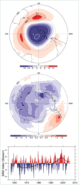
Figure 3.32. (Bottom) Seasonal values of the SAM index calculated from station data (updated from Marshall, 2003 [JoC, SRC] ). The smooth black curve shows decadal variations (see Appendix 3.A). (Top) The SAM geopotential height pattern as a regression based on the SAM time series for seasonal anomalies at 850 hPa (see also Thompson and Wallace, 2000 [JoC] ). (Middle) The regression of changes in surface temperature (°C) over the 23-year period ( 1982 to 2004 ) corresponding to a unit change in the SAM index, plotted south of 60°S. Values exceeding about 0.4°C in magnitude are significant at the 1% significance level (adapted from Kwok and Comiso, 2002b [JoC, ARC] ).
3.6.6 Atlantic Multi-decadal Oscillation
Over the instrumental period (since the 1850 s), North Atlantic SSTs show a 65 to 75 year variation (0.4°C range), with a warm phase during 1930 to 1960 and cool phases during 1905 to 1925 and 1970 to 1990 ( Schlesinger and Ramankutty, 1994 [JoC, ARC] ), and this feature has been termed the AMO ( Kerr, 2000 [JoC] ), as shown in Figure 3.33 .Evidence (e.g., Enfield et al., 2001 [JoC] ; Knight et al., 2005 [JoC] ) of a warm phase in the AMO from 1870 to 1900 is revealed as an artefact of the de-trending used ( Trenberth and Shea, 2006 [PoC, JoC, SRC] ). The cycle appears to have returned to a warm phase beginning in the mid- 1990 s, and tropical Atlantic SSTs were at record high levels in 2005 . Instrumental observations capture only two full cycles of the AMO, so the robustness of the signal has been addressed using proxies. Similar oscillations in a 60- to 110-year band are seen in North Atlantic palaeoclimatic reconstructions through the last four centuries ( Delworth and Mann, 2000 [PoC, JoC, MoS, ARC] ; Gray et al., 2004 [JoC] ). Both observations and model simulations implicate changes in the strength of the THC as the primary source of the multi-decadal variability, and suggest a possible oscillatory component to its behaviour ( Delworth and Mann, 2000 [PoC, JoC, MoS, ARC] ; Latif, 2001 [JoC, ARC] ; Sutton and Hodson, 2003 [JoC] ; Knight et al., 2005 [JoC] Trenberth and Shea 2006 [PoC, JoC, SRC] ) proposed a revised AMO index, subtracting the global mean SST from the North Atlantic SST. The revised index is about 0.35°C lower than the original after 2000, highlighting the fact that most of the recent warming is global in scale.
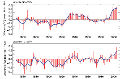
Figure 3.33. Atlantic Multi-decadal Oscillation index from 1850 to 2005 represented by annual anomalies of SST in the extratropical North Atlantic (30–65°N; top), and in a more muted fashion in the tropical Atlantic (10°N –20°N) SST anomalies (bottom). Both series come from HadSST2 ( Rayner et al., 2006 [JoC] ) and are relative to the 1961 to 1990 mean (°C). The smooth blue curves show decadal variations (see Appendix 3.A ).
The AMO has been linked to multi-year precipitation anomalies over North America, and appears to modulate ENSO teleconnections ( Enfield et al., 2001 [JoC] ; McCabe et al., 2004 [JoC] ; Shabbar and Skinner, 2004 [JoC] ). Multi-decadal variability in the North Atlantic also plays a role in Atlantic hurricane formation ( Goldenberg et al., 2001 [JoC] ; see also Section 3.8.3.2 ). The revised AMO index ( Trenberth and Shea, 2006 [PoC, JoC, SRC] ) indicates that North Atlantic SSTs have recently been about 0.3°C warmer than during 1970 to 1990, emphasizing the role of the AMO in suppressing tropical storm activity during that period. The AMO is likely to be a driver of multi-decadal variations in Sahel droughts, precipitation in the Caribbean, summer climate of both North America and Europe, sea ice concentration in the Greenland Sea and sea level pressure over the southern USA, the North Atlantic and southern Europe (e.g., Venegas and Mysak, 2000 [JoC] ; Goldenberg et al., 2001 [JoC] ; Sutton and Hodson, 2005 [JoC, MoS] ; Trenberth and Shea, 2006 [PoC, JoC, SRC] Walter and Graf 2002 [JoC] ) identified a non-stationary relationship between the NAO and the AMO. During the negative phase of the AMO, the North Atlantic SST is strongly correlated with the NAO index. In contrast, the NAO index is only weakly correlated with the North Atlantic SST during the AMO positive phase. Chelliah and Bell 2004 [JoC] ) defined a tropical multi-decadal pattern related to the AMO, the PDO and winter NAO with coherent variations in tropical convection and surface temperatures in the West African monsoon region, the central tropical Pacific, the Amazon Basin and the tropical Indian Ocean.
3.6.7 Other Indices
As noted earlier, many patterns of variability (sometimes referred to as ‘modes’) in the climate system have been identified over the years, but few stand out as robust and dynamically significant features in relation to understanding regional climate change. This section discusses two climate signals that have recently drawn the attention of scientific community: the Antarctic Circumpolar Wave and the Indian Ocean Dipole.
3.6.7.1 Antarctic Circumpolar Wave
The Antarctic Circumpolar Wave (ACW) is described as a pattern of variability with an approximately four-year period in the southern high-latitude ocean-atmosphere system, characterised by the eastward propagation of anomalies in antarctic sea ice extent, and coupled to anomalies in SST, sea surface height, MSLP and wind ( Jacobs and Mitchell, 1996 [JoC] ; White and Peterson, 1996 [JoC] ; White and Annis, 2004 [JoC] ). Since its initial formulation ( White and Peterson, 1996 [JoC] ), questions have arisen concerning many aspects of the ACW: the robustness of the ACW on inter-decadal time scales ( Carril and Navarra, 2001 [JoC] ; Connolley, 2003 [JoC] ; Simmonds, 2003 [JoC, SRC] ), its generating mechanisms ( Cai and Baines, 2001 [JoC, MoS, ARC] ; Venegas, 2003 [JoC] ; White et al., 2004 [Ambiguous] ; White and Simmonds, 2006 [JoC, SRC] ) and even its very existence ( Park et al., 2004 [JoC] ).
3.6.7.2 Indian Ocean Dipole
Large interannual variability of SST in the Indian Ocean has been associated with the Indian Ocean Dipole (IOD), also referred to as the Indian Ocean Zonal Mode (IOZM; Saji et al., 1999 [JoC] ; Webster et al., 1999 [JoC] ). This pattern manifests through a zonal gradient of tropical SST, which in one extreme phase in boreal autumn shows cooling off Sumatra and warming off Somalia in the west, combined with anomalous easterlies along the equator. The magnitude of the secondary rainfall maximum from October to December in East Africa is strongly correlated with positive IOD events ( Xie et al., 2002 [JoC, ARC] ). Several recent IOD events have occurred simultaneously with ENSO events and there is a significant debate on whether the IOD is an Indian Ocean pattern or whether it is triggered by ENSO in the Pacific Ocean ( (Allan et al., 2001 ) ). The strongest IOD episode ever observed occurred in 1997 to 1998 and was associated with catastrophic flooding in East Africa. Trenberth et al. 2002b [PoC, JoC, SRC] ) showed that Indian Ocean SSTs tend to rise about five months after the peak of ENSO in the Pacific. Monsoon variability and the SAM ( Lau and Nath, 2004 [JoC, MoS, ARC] ) are also likely to play a role in triggering or intensifying IOD events. One argument for an independent IOD was the large episode in 1961 when no ENSO event occurred ( Saji et al., 1999 [JoC] Saji and Yamagata 2003 [JoC] ), analysing observations from 1958 to 1997, concluded that 11 out of the 19 episodes identified as moderate to strong IOD events occurred independently of ENSO. However, this was disputed by ( Allan et al. 2001 ) ), who found that accounting for varying lag correlations removes the apparent independence from ENSO. Decadal variability in correlations between SST-based indices of the IOD and ENSO has been documented ( Clark et al., 2003 [JoC, ARC] ). At inter-decadal time scales, the SST patterns associated with the inter-decadal variability of ENSO indices are very similar to the SST patterns associated with the Indian monsoon rainfall ( Krishnamurthy and Goswami, 2000 [JoC] ) and with the North Pacific inter-decadal variability ( Deser et al., 2004 [JoC, SRC] ), raising the issue of coupled mechanisms modulating both ENSO-monsoon system and IOD variability (e.g., Terray et al., 2005 [JoC] ).
ENSO has exhibited considerable inter-decadal variability in the past century, in association with the PDO (or IPO). Systematic changes in ENSO behaviour have also been observed, in particular the different evolution of ENSO events and enhanced El Niño activity since the 1976 – 1977 climate shift. Over North America, ENSO- and PNA-related changes appear to have led to contrasting changes across the continent, as the west has warmed more than the east, while the latter has become cloudier and wetter. Over the Indian Ocean, ENSO, monsoon and SAM variability are related to a zonal gradient of tropical SST associated with anomalous easterlies along the equator, and opposite precipitation and thermal anomalies in East Africa and over the Maritime Continent. The tropical Pacific variability is influenced by interactions with the tropical Atlantic and Indian Oceans, and by the extratropical North and South Pacific. Responses of the extratropical ocean become more important as the time scale is extended, and processes such as subduction, gyre changes and the THC come into play.
3.6.8 Summary
Decadal variations in teleconnections considerably complicate the interpretation of climate change. Since the TAR, it has become clear that a small number of teleconnection patterns account for much of the seasonal to interannual variability in the extratropics. On monthly time scales, the SAM, NAM and NAO are dominant in the extratropics. The NAM and NAO are closely related, and are mostly independent from the SAM, except perhaps on decadal time scales. Many other patterns can be explained through combinations of the NAM and PNA in the NH, and the SAM and PSA in the SH, plus ENSO-related global patterns. Both the NAM/NAO and the SAM have exhibited trends towards their positive phase (strengthened mid-latitude westerlies) over the last three to four decades, although both have returned to near their long-term mean state in the last five years. In the NH, this trend has been associated with the observed winter change in storm tracks, precipitation and temperature patterns. In the SH, SAM changes are related to contrasting trends of strong warming in the Antarctic Peninsula and a cooling over most of interior Antarctica. The increasing positive phase of the SAM has been linked to stratospheric ozone depletion and to greenhouse gas increases. Multi-decadal variability is also evident in the Atlantic, and appears to be related to the THC. Other teleconnection patterns discussed (PNA, PSA) exhibit decadal variations, but have not been shown to have systematic long-term changes.
3.7 Changes in the Tropics and Subtropics, and in the Monsoons
The global monsoon system embraces an overturning circulation that is intimately associated with the seasonal variation of monsoon precipitation over all major continents and adjacent oceans ( Trenberth et al., 2000 [Ambiguous] ). It involves the Hadley Circulation, the zonal mean meridional overturning mass flow between the tropics and subtropics entailing the Inter-Tropical Convergence Zone (ITCZ), and the Walker Circulation, which is the zonal east-west overturning. The South Pacific Convergence Zone (SPCZ) is a semi-permanent cloud band extending from around the Coral Sea southeastward towards the extratropical South Pacific, while the South Atlantic Convergence Zone (SACZ) is a more transient feature over and southeast of Brazil that transports moisture originating over the Amazon into the South Atlantic ( Liebmann et al., 1999 [JoC] ).
Tropical SSTs determine where the upward branch of the Hadley Circulation is located over the oceans, and the dominant variations in the energy transports by the Hadley cell, reflecting its strength, relate to ENSO ( Trenberth et al., 2002a [PoC, JoC, SRC] ; Trenberth and Stepaniak, 2003a [PoC, JoC, SRC] ). During El Niño, elevated SST causes an increase in convection and relocation of the ITCZ and SPCZ to near the equator over the central and eastern tropical Pacific, with a tendency for drought conditions over Indonesia. There follows a weakening of the Walker Circulation and a strengthening of the Hadley Circulation ( Oort and Yienger, 1996 [JoC] ; Trenberth and Stepaniak, 2003a [PoC, JoC, SRC] ), leading to drier conditions over many subtropical regions during El Niño, especially over the Pacific sector. As discussed in Section 3.4.4.1 ,increased divergence of energy out of the tropics in the 1990 s relative to the 1980 s ( Trenberth and Stepaniak, 2003a [PoC, JoC, SRC] ) is associated with more frequent El Niño events and especially the major 1997 – 1998 El Niño event, so these conditions play a role in inter-decadal variability ( Gong and Ho, 2002 [JoC] ; Mu et al., 2002 [MoS] ; Deser et al., 2004 [JoC, SRC] ). Examination of the Hadley Circulation in several data sets ( Mitas and Clement, 2005 [JoC, ARC] ) suggests some strengthening, although discrepancies among reanalysis data sets and known deficiencies raise questions about the robustness of this strengthening, especially prior to the satellite era ( 1979 ).
Monsoons are generally referred to as tropical and subtropical seasonal reversals in both the surface winds and associated precipitation. The strongest monsoons occur over the tropics of southern and eastern Asia and northern Australia, and parts of western and central Africa. Rainfall is the most important monsoon variable because the associated latent heat release drives atmospheric circulations, and because of its critical role in the global hydrological cycle and its vital socioeconomic impacts. Thus, other regions that have an annual reversal in precipitation with an intense rainy summer and a dry winter have been recently recognised as monsoon regions, even though these regions have no explicit seasonal reversal of the surface winds ( Wang, 1994 [JoC, SRC] ; Webster et al., 1998 [JoC, MoS] ). The latter regions include Mexico and the southwest USA, and parts of South America and South Africa. Owing to the lack of sufficiently reliable and long-term oceanic observations, analyses of observed long-term changes have mainly relied on land-based rain gauge data.
Because the variability of regional monsoons is often the result of interacting circulations from other regions, simple indices of monsoonal strength in adjacent regions may give contradictory indications of strength ( Webster and Yang, 1992 [JoC] ; Wang and Fan, 1999 [SRC] ). Decreasing trends in precipitation over the Indonesian Maritime Continent, equatorial parts of western and central Africa, Central America, Southeast Asia and eastern Australia have been found for 1948 to 2003 ( Chen et al., 2004 [JoC] ; see Figure 3.13 ), while increasing trends were evident over the USA and northwestern Australia (see also Section 3.3.2.2 and Figure 3.14 ), consistent with Dai et al. 1997 [JoC, SRC] ). Using NRA, ( Chase et al. 2003 ) ) found diminished monsoonal circulations since 1950 and no trends since 1979, but results based on NRA suffer severely from artefacts arising from changes in the observing system ( Kinter et al., 2004 [JoC] ).
Two precipitation data sets ( Chen et al., 2002 [JoC] ; GHCN, see Section 3.3 )yield very similar patterns of change in the seasonal precipitation contrasts between 1976 to 2003 and 1948 to 1975 ( Figure 3.34 ), despite some differences in details and discrepancies in northwest India. Significant decreases in the annual range (wet minus dry season) were observed over the NH tropical monsoon regions (e.g., Southeast Asia and Central America). Over the East Asian monsoon region, the change over these periods involves increased rainfall in the Yangtze River valley and Korea but decreased rainfall over the lower reaches of the Yellow River and northeast China. In the Indonesian-Australian monsoon region, the change between the two periods is characterised by an increase in northwest Australia and Java but a decrease in northeast Australia and a northeastward movement in the SPCZ( Figure 3.34 ). However, the average monsoonal rainfall in East Asia, Indonesia-Australia and South America in summer mostly shows no long-term trend but significant interannual and inter-decadal variations. In the South African monsoon region there is a slight decrease in the annual range of rainfall( Figure 3.34 ), and a decreasing trend in area-averaged precipitation( Figure 3.14 ).
Monsoon variability depends on many factors, from regional air-sea interaction and land processes (e.g., snow cover fluctuations) to teleconnection influences (e.g., ENSO, NAO/NAM, PDO, IOD). New evidence, relevant to climate change, indicates that increased aerosol loading in the atmosphere may have strong impacts on monsoon evolution ( Menon et al., 2002 [JoC, ARC] ) through changes in local heating of the atmosphere and land surface (see also Box 3.2 and Chapter2 ).
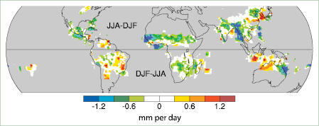
Figure 3.34. Change in the mean annual range of precipitation: 1976 to 2003 minus 1948 to 1975 periods (mm per day). Blue/green (red/yellow) colour denotes a decreasing (increasing) annual range of the monsoon rainfall. Grey areas indicate missing values (oceans) or areas with insignificant annual changes. Data were from PREC/L ( Chen et al., 2002 [JoC] ; see Wang and Ding, 2006 [JoC, SRC] ).
3.7.1 Asia
The Asian monsoon can be divided into the East Asian and the South Asian or Indian monsoon systems ( Ding et al., 2004 [ARC] ). Based on a summer monsoon index derived from MSLP gradients between land and ocean in the East Asian region, ( Guo et al. 2003 ) ) found a systematic reduction in the East Asian summer monsoon during 1951 to 2000, with a stronger monsoon dominant in the first half of the period and a weaker monsoon prevailing in the second half( Figure 3.35 ). This long-term change in the East Asian monsoon index is consistent with a tendency for a southward shift of the summer rain belt over eastern China ( Zhai et al., 2004 [JoC] ). However, Figure 3.35 ,based on the newly developed Hadley Centre MSLP data set version 2 (HadSLP2; Allan and Ansell, 2006 [JoC, SRC] ), suggests that although there exists a weakening trend starting in the 1920 s, it is not reflected in the longer record extending back to the 1850 s, which shows marked decadal-scale variability before the 1940 s.
There is other evidence that changes in the Asian monsoon occurred about the time of the 1976 – 1977 climate shift ( (Wang, 2001 ) ) along with changes in ENSO ( Huang et al., 2003 [ARC] ; Qian et al., 2003 [JoC] ), and declines in land precipitation are evident in southern Asia and, to some extent, in Southeast Asia (see Figure 3.14 Gong and Ho 2002 [JoC] ) suggested that the change in summer rainfall over the Yangtze River valley was due to a southward rainfall shift and Ho et al. 2003 [JoC] ) noted a sudden change in Korea. These occurred about the same time as a change in the 500 hPa geopotential height and typhoon tracks in summer over the northern Pacific ( Gong et al., 2002 [Ambiguous] ; see Section 3.6.3 )related to the enlargement, intensification and southwestward extension of the northwest Pacific subtropical high. When the equatorial central and eastern Pacific is in a decadal warm period, summer monsoon rainfall is stronger in the Yangtze River valley but weaker in North China. A strong tropospheric cooling trend is found in East Asia during July and August. Accompanying this summer cooling, the upper-level westerly jet stream over East Asia shifts southward and the East Asian summer monsoon weakens, which results in the tendency towards increased droughts in northern China and floods in the Yangtze River valley ( Yu et al., 2004b [JoC, SRC] ).
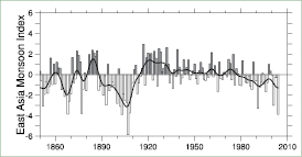
Figure 3.35. Annual values of the East Asia summer monsoon index derived from MSLP gradients between land and ocean in the East Asia region. The definition of the index is based on ( Guo et al. 2003 ) ) but was recalculated based on the HadSLP2 ( Allan and Ansell, 2006 [JoC, SRC] ) data set. The smooth black curve shows decadal variations (see Appendix 3.A ).
Rainfall during the Indian monsoon season, which runs from June to September and accounts for about 70% of annual rainfall, exhibits decadal variability. Observational studies have shown that the impact of El Niño is more severe during the below-normal epochs, while the impact of la Niña is more severe during the above-normal epochs ( Kripalani and Kulkarni, 1997a [SRC] ; Kripalani et al., 2001 [Ambiguous] , 2003 ). Such modulation of ENSO impacts by the decadal monsoon variability was also observed in the rainfall regimes over Southeast Asia ( Kripalani and Kulkarni, 1997b [JoC, SRC] ). Links between monsoon-related events (rainfall over South Asia, rainfall over East Asia, NH circulation, tropical Pacific circulation) weakened between 1890 and 1930 but strengthened during 1930 to 1970 ( Kripalani and Kulkarni, 2001 [JoC, SRC] ). The strong inverse relationship between El Niño events and Indian monsoon rainfalls that prevailed for more than a century prior to about 1976 has weakened substantially since then ( Kumar et al., 1999 [JoC] ; Krishnamurthy and Goswami, 2000 [JoC] ; Sarkar et al., 2004 [JoC] ), involving large-scale changes in atmospheric circulation. Shifts in the Walker Circulation and enhanced land-sea contrasts appear to be countering effects of increased El Niño activity. Ashok et al. 2001 [JoC] ) also found that the IOD (see Section 3.6.7.2 )plays an important role as a modulator of Indian rainfall. The El Niño-Southern Oscillation is also related to atmospheric fluctuations both in the Indian sector and in northeastern China ( Kinter et al., 2002 [JoC] ).
3.7.2 Australia
The Australian monsoon covers the northern third of continental Australia and surrounding seas and, considering its closely coincident location and annual evolution, is often studied in conjunction with the monsoon over the islands of Indonesia and Papua New Guinea. The Australian monsoon exhibits large interannual and intra-seasonal variability, largely associated with the effects of ENSO, the Madden-Julian Oscillation (MJO) and tropical cyclone activity ( McBride, 1998 [NPR] ; Webster et al., 1998 [JoC, MoS] ; Wheeler and McBride, 2005 [NPR, SRC] ). Using rain-gauge data, Hennessy et al. 1999 [ARC] ) found an increase in calendar-year total rainfall in the Northern Territory of 18% from 1910 to 1995, attributed mostly to enhanced monsoon rainfall in the 1970 s and coincident with an almost 20% increase in the number of rain days. With data updated to 2002, ( Smith 2004 ) ) demonstrated that increased monsoon rainfall has become statistically significant over northern, western and central Australia. Northern Australian wet season rainfall ( (Jones et al., 2004 ) ), updated through 2004 – 2005 ( Figure 3.36 ), shows the positive trend and the contribution of the anomalously wet period of the mid- 1970 s as well as the more recent anomalously wet period around 2000 (see also ( Smith, 2004 ) Wardle and Smith 2004 [JoC, MoS] ) argued that the upward rainfall trend is consistent with the upward trend in land surface temperatures that has been observed in the south of the continent, independent of changes over the oceans. Strong decadal variations in Australian precipitation have also been noted( Figure 3.36 ). Using northeastern Australian rainfall, Latif et al. 1997 [JoC, ARC] ) showed that rainfall was much increased during decades when the tropical Pacific was anomalously cold (the 1950 s and 1970 s). This strong relationship does not extend to the Australian monsoon as a whole, however, as the rainfall time series( Figure 3.36 )has only a weak negative correlation (approximately –0.2) with the IPO. The fact that the long-term trends in rainfall and Pacific SSTs are both positive, the opposite of their interannual relationship ( Power et al., 1998 [ARC] ), explains only a portion of why the correlation is reduced at decadal time scales.
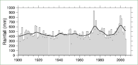
Figure 3.36. Time series of northern Australian (north of 26°S) wet season (October–April) rainfall (mm) from 1900 / 1901 to 2004 / 2005 . The individual bar corresponds to the January of the summer season (e.g., 1990 is the summer of 1989 / 1990 ). The smooth black curve shows decadal variations (see Appendix 3.A ). Data from the Australian Bureau of Meteorology.
3.7.3 The Americas
The North American Monsoon System (NAMS) is characterised by ocean-land contrasts including summer heating of higher-elevation mountain and plateau regions of Mexico and the southwestern USA, a large-scale upper-level anticyclonic circulation, a lower-level thermal low and a strong subsidence region to the west in the cool stratus regime of the eastern North Pacific ( Vera et al., 2006 [JoC] ). The NAMS contains a strong seasonal structure ( Higgins and Shi, 2000 [JoC] ), with rapid onset of monsoon rains in southwestern Mexico in June, a later northward progression into the southwest USA during its mature phase in July and August and a gradual decay in September and October.
Timing of the start of the northern portion of the NAMS has varied considerably, with some years starting as early as mid-June and others starting as late as early August ( Higgins and Shi, 2000 [JoC] ). Since part of NAMS variability is governed by larger-scale climate conditions, it is susceptible to interannual and multi-decadal variations. Higgins and Shi 2000 [JoC] ) further suggested that the northern portion of the NAMS may be affected by the PDO, wherein anomalous winter precipitation over western North America is correlated with North American monsoon conditions in the subsequent summer.
The South American Monsoon System (SAMS) is evident over South America in the austral summer ( (Barros et al., 2002; ) ( Nogués-Paegle et al., 2002; ) Vera et al., 2006 [JoC] ). It is a key factor for the warm season precipitation regime. In northern Brazil, different precipitation trends (see Figure 3.14 for the Amazon and southern South America regions) have been observed over northern and southern Amazonia, showing a dipole structure ( Marengo, 2004 [Ambiguous] ) that suggests a southward shift of the SAMS. This is consistent with Rusticucci and Penalba 2000 [ARC] ), who found a significant positive trend in the amplitude of the annual precipitation cycle, indicating a long-term climate change of the monsoon regime over the semi-arid region of the la Plata Basin. In addition, the mean wind speed of the low-level jet, a component of the SAMS that transports moisture from the Amazon to the south and southwest, showed a positive trend ( Marengo et al., 2004 [Ambiguous] ). Positive SST anomalies in the western subtropical South Atlantic are associated with positive rainfall anomalies over the SACZ region ( Doyle and Barros, 2002 [JoC] ; Robertson et al., 2003 [JoC] ( Barros et al. 2000b ) ) found that, during summer, the SACZ was displaced northward (southward) and was more intense (weaker) with cold (warm) SST anomalies to its south. The convergence zone is modulated in part by surface features, including the gradient of SST over the equatorial Atlantic ( Chang et al., 1999 [JoC] ;( Nogués-Paegle et al., 2002 ) ), and it modulates the interannual variability of seasonal rainfall over eastern Amazonia and northeastern Brazil ( Nobre and Shukla, 1996 [JoC, ARC] ; Folland et al., 2001 [PoC, JoC, MoS, SRC] ).
3.7.4 Africa
Since the TAR, a variety of studies have firmly established that ENSO and SSTs in the Indian Ocean are the dominant sources of climate variability over eastern Africa ( Goddard and Graham, 1999 [JoC, MoS] ; Yu and Rienecker, 1999 [JoC] ; Indeje et al., 2000 [JoC, ARC] ; Clark et al., 2003 [JoC, ARC] ). Further, Schreck and Semazzi 2004 [NotFound] ) isolated a secondary but significant pattern of regional climate variability based on seasonal (OND) rainfall data. In distinct contrast to the ENSO-related spatial pattern, the trend pattern in their analysis is characterised by positive rainfall anomalies over the northeastern sector of eastern Africa (Ethiopia, Somalia, Kenya and northern Uganda) and opposite conditions over the southwestern sector (Tanzania, southern parts of the Democratic Republic of the Congo and southwestern Uganda). This signal significantly strengthened in recent decades. Warming is associated with an earlier onset of the rainy season over the northeastern Africa region and a late start over the southern sector.
West Africa experiences marked multi-decadal variability in rainfall (e.g., le Barbe et al., 2002 [JoC] ; Dai et al., 2004b [JoC, SRC] ). Wet conditions in the 1950 s and 1960 s gave way to much drier conditions in the 1970 s, 1980 s and 1990 s. The rainfall deficit in this region during 1970 to 1990 was relatively uniform across the region, implying that the deficit was not due to a spatial shift in the peak rainfall ( Le Barbe et al., 2002 [JoC] ) and was mainly linked to a reduction in the number of significant rainfall events occurring during the peak monsoon period (JAS) in the Sahel and during the first rainy season south of about 9°N. The decreasing rainfall and devastating droughts in the Sahel region during the last three decades of the 20th century( Figure 3.37 )are among the largest climate changes anywhere. Dai et al. 2004b [JoC, SRC] ) provided an updated analysis of the normalised Sahel rainfall index based on the years 1920 to 2003 ( Figure 3.37 ). Following the major 1982 – 1983 El Niño event, rainfall reached a minimum of 170 mm below the long-term mean of about 506 mm. Since 1982, there is some evidence for a recovery (see also lower panel of Figure 3.13 )but despite this, the mean of the last decade is still well below the pre- 1970 level. These authors also noted that large multi-year oscillations appear to be more frequent and extreme after the late 1980 s than previously.
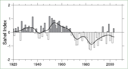
Figure 3.37. Time series of Sahel (10ºN –20ºN, 18ºW–20ºE) regional rainfall (April–October) from 1920 to 2003 derived from gridding normalised station anomalies and then averaging using area weighting (adapted from Dai et al., 2004a [JoC] ). The smooth black curve shows decadal variations (see Appendix 3.A ).
ENSO affects the West African monsoon, and the correlation between Sahel rainfall and ENSO during JJA varied between 1945 and 1993 ( Janicot et al., 2001 [JoC] ). The correlation was always negative but was not significant during the 1960 s to the mid- 1970 s when the role of the tropical Atlantic was relatively more important. Years when ENSO has a larger impact tend to be associated with same-signed rainfall anomalies over the West African region whereas years when the tropical Atlantic is more important tend to have a so-called anomalous ‘dipole’ pattern, with the Sahel and Guinea Coast having opposite-signed rainfall anomalies ( Ward, 1998 [JoC, MoS] Giannini et al. 2003 [JoC, MoS] ) suggested that both interannual and decadal variability of Sahel rainfall results from the response of the African summer monsoon to oceanic forcing, amplified by land-atmosphere interaction.
While other parts of Africa have experienced statistically significant weakening of the monsoon circulation, analyses of long-term southern African rainfall totals in the wet season (JFM) have reported no trends ( (Fauchereau et al., 2003 ) ). Decreases in rainfall are evident in analyses of shorter periods, such as the decade from 1986 to 1995 that was the driest of the 20th century. New et al. 2006 [JoC, ARC] ) reported a decrease in average rainfall intensity and an increase in dry spell length (number of consecutive dry days) for 1961 to 2000 .
3.7.5 Summary
Variability at multiple time scales strongly affects monsoon systems. Large interannual variability associated with ENSO dominates the Hadley and Walker Circulations, the ITCZ and monsoons. There is also good evidence for decadal changes associated with monsoonal rainfall changes in many monsoon systems, especially across the 1976 – 1977 climate shift, but data uncertainties compromise evidence for trends. Some monsoons, especially the East Asian monsoon system, have experienced a dipole change in precipitation with increases in one region and decreases in the other during the last 50 years.
3.8 Changes in Extreme Events
3.8.1 Background
There is increasing concern that extreme events may be changing in frequency and intensity as a result of human influences on climate. Climate change may be perceived most through the impacts of extremes, although these are to a large degree dependent on the system under consideration, including its vulnerability, resiliency and capacity for adaptation and mitigation; see the Working Group II contribution to the IPCC Fourth Assessment Report. Improvements in technology mean that people hear about extremes in most parts of the world within a few hours of their occurrence. Pictures shot by camcorders on the news may foster a belief that weather-related extremes are increasing in frequency, whether they are or not. An extreme weather event becomes a disaster when society and/or ecosystems are unable to cope with it effectively. Growing human vulnerability (due to growing numbers of people living in exposed and marginal areas or due to the development of more high-value property in high-risk zones) is increasing the risk, while human endeavours (such as by local governments) try to mitigate possible effects.
The assessment of extremes in this section is based on long-term observational series of weather elements. As in the TAR, extremes refer to rare events based on a statistical model of particular weather elements, and changes in extremes may relate to changes in the mean and variance in complicated ways. Changes in extremes are assessed at a range of temporal and spatial scales, for example, from extremely warm years globally to peak rainfall intensities locally, and examples are given in Box 3.6 .To span this entire range, data are required at a daily (or shorter) time scale. However, the availability of observational data restricts the types of extremes that can be analysed. The rarer the event, the more difficult it is to identify long-term changes, simply because there are fewer cases to evaluate ( Frei and Schär, 2001 [JoC, SRC] ; Klein Tank and Können, 2003 [JoC] ). Identification of changes in extremes is also dependent on the analysis technique employed ( Zhang et al., 2004a [JoC, MoS, ARC] ;( Trömel and Schönwiese, 2005 ) ). To avoid excessive statistical limitations, trend analyses of extremes have traditionally focused on standard and robust statistics that describe moderately extreme events. In percentile terms, these are events occurring between 1 and 10% of the time at a particular location in a particular reference period (generally 1961 to 1990 ). Unless stated otherwise, this section focuses on changes in these extremes.
Global studies of daily temperature and precipitation extremes over land (e.g., ( Frich et al., 2002; ) see also the TAR) suffer from both a scarcity of data and regions with missing data. The main reason is that in various parts of the globe there is a lack of homogeneous observational records with daily | resolution covering multiple decades that are part of integrated digitised data sets ( GCOS, 2003 [NPR] ). In addition, existing records are often inhomogeneous; for instance as a result of changes in observing practices or UHI effects (DeGaetano and Allen, 2002 [JoC, MoS, ARC] ;( Vincent et al., 2002; ) Wijngaard et al., 2003 [JoC] ). This affects, in particular, the understanding of extremes, because changes in extremes are often more sensitive to inhomogeneous climate monitoring practices than changes in the mean (see Appendix 3.B.2 and 3.B.4). Consistent observing is also a problem when assessing long-term changes in the frequency and severity of tropical and extratropical storms. Similar difficulties are encountered when trying to find worldwide observational evidence for changes in severe local weather events like tornadoes, hail, thunderstorms and dust storms. Analyses of trends in extremes are also sensitive to the analysis period, for example, the inclusion of the exceptionally hot European summer of 2003 may have a marked influence on results if the period is short.
Since the TAR, the situation with observational data sets has improved, although efforts to update and exchange data must be continued (e.g., GCOS, 2004 [NPR] ). Results are now available from newly established regional- and continental-scale daily data sets; from denser networks, from temporally more extended high-quality time series and from many existing national data archives, which have been expanded to cover longer time periods. Moreover, the systematic use and exchange of time series of standard indices of extremes, with common definitions, provides an unprecedented global picture of changes in daily temperature and precipitation extremes ( Alexander et al., 2006 [JoC, SRC] , updating the results of ( Frich et al., 2002 ) presented in the TAR).
As an alternative, but not independent data source, reanalyses can also be analysed for changes in extremes (see Appendix 3.B.5.4). Although spatially and temporally complete, under-representation of certain types of extremes ( Kharin and Zwiers, 2000 [JoC, MoS, ARC] ) and spurious trends in the reanalyses (especially in the tropics and in the SH) remain problematic, in particular before the start of the modern satellite era in 1979 ( Marshall, 2002 [JoC, SRC] , 2003; Sturaro, 2003 [JoC] ; Sterl, 2004 [JoC] ; Trenberth et al., 2005a [PoC, JoC, SRC] ). For instance, Bengtsson et al. 2004 [JoC, ARC] ) found that analysed global kinetic energy rose by almost 5% in 1979 as a direct consequence of the inclusion of improved satellite information over the oceans, which is expected to significantly affect analysed storm activity over the southern oceans, where ship data are sparse.
In this section, observational evidence for changes in extremes is assessed for temperature, precipitation, tropical and extratropical cyclones and severe local weather events. Most studies of extremes consider the period since about 1950 with even greater emphasis on the last few decades (since 1979 ), although longer data sets exist for a few regions, enabling more recent events to be placed in a longer context. The section discusses mostly the changes observed in the daily weather elements, where most progress has been made since the TAR. Droughts (although they are considered extremes) are covered in Section 3.3.4 as they are more related to longer periods of anomalous climate.
3.8.2 Evidence for Changes in Variability or Extremes
3.8.2.1 Temperature
For temperature extremes in the 20th century, the TAR highlighted the lengthening of the growing or frost-free season in most mid- and high-latitude regions, a reduction in the frequency of extreme low monthly and seasonal average temperatures and smaller increases in the frequency of extreme high average temperatures. In addition, there was evidence to suggest a decrease in the intra-annual temperature variability with consistent reductions in frost days and increases in warm nighttime temperatures across much of the globe.
Evidence for changes in observed interannual variability (such as standard deviations of seasonal averages) is still sparse. Scherrer et al. 2005 [JoC, ARC] ) investigated standardised distribution changes for seasonal mean temperature in central Europe and found that temperature variability showed a weak increase (decrease) in summer (winter) for 1961 to 2004, but these changes are not statistically significant at the 10% level. On the daily time scale, regional studies have been completed for southern South America ( Vincent et al., 2005 [JoC] ), Central America and northern South America ( Aguilar et al., 2005 [JoC] ), the Caribbean ( Peterson et al., 2002 [JoC, ARC] ), North America ( Kunkel et al., 2004 [JoC, SRC] ;( Vincent and Mekis, 2006 ) ), the Arctic ( Groisman et al., 2003 [NPR, SRC] ), central and northern Africa ( Easterling et al., 2003 [JoC, SRC] ), southern and western Africa ( New et al., 2006 [JoC, ARC] ), the Middle East ( Zhang et al., 2005 [JoC, ARC] ), Western Europe and east Asia ( Kiktev et al., 2003 [PoC, JoC, MoS, SRC] ), Australasia and southeast Asia ( Griffiths et al., 2005 [JoC, MoS] ), China ( Zhai and Pan, 2003 [JoC] ) and central and southern Asia ( Klein Tank et al., 2006 [JoC] ). They all show patterns of changes in extremes consistent with a general warming, although the observed changes of the tails of the temperature distributions are often more complicated than a simple shift of the entire distribution would suggest (see Figure 3.38 ). In addition, uneven trends are observed for nighttime and daytime temperature extremes. In southern South America, significant increasing trends were found in the occurrence of warm nights and decreasing trends in the occurrence of cold nights, but no consistent changes in the indices based on daily maximum temperature. In Central America and northern South America, high extremes of both minimum and maximum temperature have increased. Warming of both the nighttime and daytime extremes was also found for the other regions where data have been analysed. For Australasia and Southeast Asia, the dominant distribution change at rural stations for both maximum and minimum temperature involved a change in the mean, affecting either one or both distribution tails, with no significant change in standard deviation ( Griffiths et al., 2005 [JoC, MoS] ). For urbanised stations, however, the dominant change also involved a change in the standard deviation. This result was particularly evident for minimum temperature.
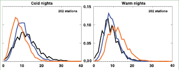
Figure 3.38. Annual probability distribution functions for temperature indices for 202 global stations with at least 80% complete data between 1901 and 2003 for three time periods: 1901 to 1950 (black), 1951 to 1978 (blue) and 1979 to 2003 (red). The x-axis represents the percentage of time during the year when the indicators were below the 10th percentile for cold nights (left) or above the 90th percentile for warm nights (right). From Alexander et al. 2006 [JoC, SRC] ).
Few other studies have considered mutual changes in both the high and low tail of the same daily (minimum, maximum or mean) temperature distribution. Klein Tank and Können 2003 [JoC] ) analysed such changes over Europe using standard indices, and found that the annual number of warm extremes (above the 90th percentile for 1961 to 1990 ) of the daily minimum and maximum temperature distributions increased twice as fast during the last 25 years than expected from the corresponding decrease in the number of cold extremes (lowest 10%). Moberg and Jones 2005 [JoC, SRC] ) found that both the high and the low tail (defined by the 90th and 10th percentile) of the daily minimum and maximum temperature distribution over Europe in winter increased over the 20th century as a whole, with the low tail of minimum temperature warming significantly in summer. For an even longer period, Yan et al. 2002 [JoC] ) found decreasing warm extremes in Europe and China up to the late 19th century, decreasing cold extremes since then, and increasing warm extremes only since 1961, especially in summer (JJA). Brunet et al. 2006 [JoC] ) analysed 22 Spanish records for the period 1894 to 2003 and found greater reductions in the number of cold days than increases in hot days. However, since 1973 warm days have been rising dramatically, particularly near the Mediterranean coast. Beniston and Stephenson 2004 [JoC, SRC] ) showed that changes in extremes of daily temperature in Switzerland were due to changes in both the mean and the variance of the daily temperatures. ( Vincent and Mekis 2006 ) ) found progressively fewer extreme cold nights and cool days but more extreme warm nights and hot days for Canada from 1900 to 2003 and Robeson 2004 [JoC] ) found intense warming of the lowest daily minimum temperatures over western and central North America. In Argentina, the strong positive changes in minimum temperature seen during 1959 to 1998 were associated with significant increases in the frequency of warm nights; there were also decreases in cold days ( Rusticucci and Barrucand, 2004 [JoC, ARC] ).
Alexander et al. 2006 [JoC, SRC] and Caesar et al. 2006 [JoC, SRC] ) have brought all these and other regional results together, gridding the common indices or data for the period since 1946 . Over 74% of the global land area sampled showed a significant decrease in the annual occurrence of cold nights; a significant increase in the annual occurrence of warm nights took place over 73% of the area( Table 3.6 , Figure 3.38 and FAQ 3.3 ). This implies a positive shift in the distribution of daily minimum temperatureTmin throughout the globe. Changes in the occurrence of cold and warm days show warming as well, but generally less marked. This is consistent withTmin increasing more than maximum temperatureTmax,leading to a reduction in DTR since 1951 (see Sections 3.2.2.1 and 3.2.2.7 ). The change in the four extremes indices( Table 3.6 )also show that the distribution ofTmin andTmax have not only shifted, but also changed in shape. The indices for the number of cold and warm events have changed almost equally, which for a near-Gaussian distributed quantity indicates that the cold tails of the distributions have warmed considerably more than the warm tails over the last 50 years. Considering the last 25 years only, such a change in shape is not seen( Table 3.6 ).
3.8.2.2 Precipitation
The conceptual basis for changes in precipitation has been given by Allen and Ingram 2002 [JoC, MoS, ARC] and Trenberth et al. 2003 [PoC, JoC, SRC] ; see Section 3.3 and FAQ 3.2 ). Issues relate to changes in type, amount, frequency, intensity and duration of precipitation. Observed increases in atmospheric water vapour (see Section 3.4.2 )imply increases in intensity, but this will lead to reduced frequency or duration if the total evaporation rate from the Earth’s surface (land and ocean) is unchanged. The TAR states that it is likely that there has been a statistically significant 2 to 4% increase in the frequency of heavy and extreme precipitation events when averaged across the middle and high latitudes. Since then a more refined understanding of the observed changes in precipitation extremes has been achieved.
Many analyses indicate that the evolution of rainfall statistics through the second half of the 20th century is dominated by variations on the interannual to inter-decadal time scale and that trend estimates are spatially incoherent ( Manton et al., 2001 [JoC] ; Peterson et al., 2002 [JoC, ARC] ; Griffiths et al., 2003 [JoC] ; Herath and Ratnayake, 2004 [JoC, MoS] ). In Europe, there is a clear majority of stations with increasing trends in the number of moderately and very wet days (defined as wet days (≥1 mm of rain) that exceed the 75th and 95th percentiles, respectively) during the second half of the 20th century ( Klein Tank and Können, 2003 [JoC] ; Haylock and Goodess, 2004 [JoC] ). Similarly, for the contiguous USA, Kunkel et al. 2003 [JoC, SRC] and Groisman et al. 2004 [JoC, SRC] ) confirmed earlier results and found statistically significant increases in heavy (upper 5%) and very heavy (upper 1%) precipitation of 14 and 20%, respectively. Much of this increase occurred during the last three decades of the 20th century and is most apparent over the eastern parts of the country. In addition, there is new evidence from Europe and the USA that the relative increase in precipitation extremes is larger than the increase in mean precipitation, and this is manifested as an increasing contribution of heavy events to total precipitation ( Klein Tank and Können, 2003 [JoC] ; Groisman et al., 2004 [JoC, SRC] ).
Despite a decrease in mean annual rainfall, an increase in the fraction from heavy events was inferred for large parts of the Mediterranean ( Alpert et al., 2002 [JoC] ; Brunetti et al., 2004 [JoC] ; Maheras et al., 2004 [JoC] ). Further, Kostopoulou and Jones 2005 [SRC] ) noted contrasting trends of heavy rainfall events between an increase in the central Mediterranean (Italy) and a decrease over the Balkans. In South Africa, Siberia, central Mexico, Japan and the northeastern part of the USA, an increase in heavy precipitation was also observed, while total precipitation and/or the frequency of days with an appreciable amount of precipitation (wet days) was either unchanged or decreasing ( Easterling et al., 2000 [ARC] ;( Fauchereau et al., 2003; ) Sun and Groisman, 2004 [JoC, SRC] ; Groisman et al., 2005 [SRC] ).
Anumber of recent regional studies have been completed for southern South America ( Haylock et al., 2006 [JoC] ), Central America and northern South America ( Aguilar et al., 2005 [JoC] ), southern and western Africa ( New et al., 2006 [JoC, ARC] ), the Middle East ( Zhang et al., 2005 [JoC, ARC] ) and central and southern Asia ( Klein Tank et al., 2006 [JoC] ). For southern South America, the pattern of trends for extremes between 1960 and 2000 was generally the same as that for total annual rainfall ( Haylock et al., 2006 [JoC] ). A majority of stations showed a change to wetter conditions, related to the generally lower value of the SOI since 1976 / 1977, with the exception of southern Peru and southern Chile, where a decrease was observed in many precipitation indices. In the latter region, the change in ENSO has led to a weakening of the continental trough resulting in a southward shift in storm tracks and an important effect on the observed rainfall trends. No significant increases in total precipitation amounts were found over Central America and northern South America (see also Figure 3.14 ), but rainfall intensities have increased related to changes in SST of tropical Atlantic waters. Over southern and western Africa, and the Middle East, there are no spatially coherent patterns of statistically significant trends in precipitation indices. Averaged over central and southern Asia, a slight indication of disproportionate changes in the precipitation extremes compared with the total amounts is seen. In the Indian sub-continent Sen Roy and Balling 2004 [JoC] ) found that about two- thirds of all considered time series exhibit increasing trends in indices of precipitation extremes and that there are coherent regions with increases and decreases.
Alexander et al. 2006 [JoC, SRC] ) also gridded the extreme indices for precipitation (as for temperature in Section 3.8.2.1 ). Changes in precipitation extremes are much less coherent than for temperature, but globally averaged over the land area with sufficient data, the percentage contribution to total annual precipitation from very wet days (upper 5%) is greater in recent decades than earlier decades( Figure 3.39 ,top panel, and Table 3.6 ,last line). Observed changes in intense precipitation (with geographically varying thresholds between the 90th and 99.9th percentile of daily precipitation events) for more than one half of the global land area indicate an increasing probability of intense precipitation events beyond that expected from changes in the mean for many extratropical regions ( Groisman et al., 2005 [SRC] ; Figure 3.39 ,bottom panel). This finding supports the disproportionate changes in the precipitation extremes described in the majority of regional studies above, in particular for the mid-latitudes since about 1950 . It is still difficult to draw a consistent picture of changes in the tropics and the subtropics, where many areas are not analysed and data are not readily available.
Table 3.6. Global trends in extremes of temperature and precipitation as measured by the 10th and 90th percentiles (for 1961 – 1990 ). Trends with 5 and 95% confidence intervals and levels of significance (bold: <1%) were estimated by REML (see Appendix 3.A ), which allows for serial correlation in the residuals of the data about the linear trend. All trends are based on annual averages. Values are % per decade. Based on Alexander et al. 2006 [JoC, SRC] ).
| Trend (% per decade) | ||
|---|---|---|
| Series | 1951–2003 | 1979–2003 |
| TN10: % incidence ofTmin below coldest decile. | −1.17 ± 0.20 | −1.24 ± 0.44 |
| TN90: %incidence ofTmin above warmest decile. | 1.43 ± 0.42 | 2.60 ± 0.81 |
| TX10: %incidence ofTmax below coldest decile. | −0.63 ± 0.16 | −0.91 ± 0.48 |
| TX90: %incidence ofTmax above warmest decile. | 0.71 ± 0.35 | 1.74 ± 0.72 |
| PREC:% contribution of very wet days (above the 95thpercentile) to the annual precipitation total. | 0.21 ± 0.10 | 0.41 ± 0.38 |
As well as confirming previous findings, the new analyses provide seasonal detail and insight into longer-term variations for the mid-latitudes. While the increase in the USA is found primarily in the warm season ( Groisman et al., 2004 [JoC, SRC] ), central and northern Europe exhibited changes primarily in winter (DJF) and changes were insignificant in summer (JJA), but the studies did not include the extreme European summers of 2002 (very wet) and 2003 (very dry) ( Osborn and Hulme, 2002 [PoC, JoC, ARC] ; Haylock and Goodess, 2004 [JoC] ; Schmidli and Frei, 2005 [JoC, SRC] ). Although data are not as good, the frequencies of precipitation extremes in the USA were at comparable levels from 1895 into the early 1900 s and during the 1980 s to 1990 s ( Kunkel et al., 2003 [JoC, SRC] ). For Canada (excluding the high-latitude Arctic), Zhang et al. 2001a [JoC, ARC] ( and Vincent and Mekis 2006 ) ) found that the frequency of precipitation days significantly increased during the 20th century, but averaged for the country as a whole, there is no identifiable trend in precipitation extremes. Nevertheless, Groisman et al. 2005 [SRC] ) found significant increases in the frequency of heavy and very heavy (between the 95th and 99.7th percentile of daily precipitation events) precipitation in British Columbia south of 55°N for 1910 to 2001, and in other areas( Figure 3.39 ,bottom panel).
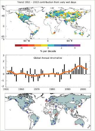
Figure 3.39. (Top) Observed trends (% per decade) for 1951 to 2003 in the contribution to total annual precipitation from very wet days (95th percentile). Trends were only calculated for grid boxes where both the total and the 95th percentile had at least 40 years of data during this period and had data until at least 1999 . (Middle) Anomalies (%) of the global annual time series (with respect to 1961 to 1990 ) defined as the percentage change of contributions of very wet days from the base period average (22.5%). The smooth red curve shows decadal variations (see Appendix 3.A ). From Alexander et al. 2006 [JoC, SRC] ). (Bottom) Regions where disproportionate changes in heavy and very heavy precipitation during the past decades were documented as either an increase (+) or decrease (–) compared to the change in the annual and/or seasonal precipitation (updated from Groisman et al., 2005 [SRC] ). Thresholds used to define “heavy” and “very heavy” precipitation vary by season and region. However, changes in heavy precipitation frequencies are always greater than changes in precipitation totals and, in some regions, an increase in heavy and/or very heavy precipitation occurred while no change or even a decrease in precipitation totals was observed.
Since the TAR, several regional analyses have been undertaken for statistics with return periods much longer than in the previous studies. For the UK, Fowler and Kilsby 2003a [JoC] ,b), using extreme value statistics, estimated that the recurrence of 10-day precipitation totals with a 50-year return period (based on data for 1961 to 1990 ) had increased by a factor of two to five by the 1990 s in northern England and Scotland. Their results for long return periods are qualitatively similar to changes obtained for traditional (moderate) statistics ( Osborn et al., 2000 [PoC, JoC, ARC] ; Osborn and Hulme, 2002 [PoC, JoC, ARC] ), but there are differences in the relative magnitude of the change between seasons ( Fowler and Kilsby, 2003b [JoC] ). For the contiguous USA, Kunkel et al. 2003 [JoC, SRC] and Groisman et al. 2004 [JoC, SRC] ) analysed return periods of 1 to 20 years, and interannual to inter-decadal variations during the 20th century exhibit a high correlation between all return periods. Similar results were obtained for several extratropical regions ( Groisman et al., 2005 [SRC] ), including the central USA, the northwestern coast of North America, southern Brazil, Fennoscandia, the East European Plain, South Africa, southeastern Australia and Siberia. In summary, from the available analyses there is evidence that the changes at the extreme tail of the distribution (several-decade return periods) are consistent with changes inferred for more robust statistics based on percentiles between the 75th and 95th levels, but practically no regions have sufficient data to assess such trends reliably.
3.8.3 Evidence for Changes in Tropical Storms
The TAR noted that evidence for changes in tropical cyclones (both in number and in intensity) across the various ocean basins is often hampered by classification changes. In addition, considerable inter-decadal variability reduces significance of any long-term trends. Careful interpretation of observational records is therefore required. Traditional measures of tropical cyclones, hurricanes and typhoons have varied in different regions of the globe, and typically have required thresholds of estimated wind speed to be crossed for the system to be called a tropical storm, named storm, cyclone, hurricane or typhoon, or major hurricane or super typhoon. Many other measures or terms exist, such as ‘named storm days’, ‘hurricane days’, ‘intense hurricanes’, ‘net tropical cyclone activity’, and so on.
The ACE index (see Box 3.5 ), is essentially a wind energy index, defined as the sum of the squares of the estimated six-hour maximum sustained wind speed (knots) for all named systems while they are at least tropical storm strength. Since this index represents a continuous spectrum of both system duration and intensity, it does not suffer as much from the discontinuities inherent in more widely used measures of activity such as the number of tropical storms, hurricanes or major hurricanes. However, the ACE values reported here are not adjusted for known inhomogeneities in the record (discussed below). The ACE index is also used to define above-, near-, and below-normal hurricane seasons (based on the 1981 to 2000 period). The index has the same meaning in every region. Figure 3.40 shows the ACE index for six regions (adapted from Levinson, 2005 [JoC, SRC] , and updated through early 2006 ). Prior to about 1970, there was no satellite imagery to help estimate the intensity and size of tropical storms, so the estimates of ACE are less reliable, and values are not given prior to about the mid- or late 1970 s in the Indian Ocean, South Pacific or Australian regions. Values are given for the Atlantic and two North Pacific regions after 1948, although reliability improves over time, and trends contain unquantified uncertainties.
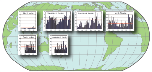
Figure 3.40. Seasonal values of the ACE index for the North Indian, South Indian, West North Pacific, East North Pacific, North Atlantic and combined Australian-South Pacific regions. The vertical scale in the West North Pacific is twice as large as that of other basins. The SH values are those for the season from July the year before to June of the year plotted. The timeline runs from 1948 or 1970 through 2005 in the NH and through June 2006 in the SH. The ACE index accounts for the combined strength and duration of tropical storms and hurricanes during a given season by computing the sum of squares of the six-hour maximum sustained surface winds in knots while the storm is above tropical storm intensity. Adapted and updated from Levinson 2005 [JoC, SRC] ).
The Potential Intensity (PI) of tropical cyclones ( (Emanuel, 2003 ) ) can be computed from observational data based primarily on vertical profiles of temperature and humidity (see Box 3.5 )and on SSTs. In analysing CAPE (see Box 3.5 )from selected radiosonde stations throughout the tropics for the period 1958 to 1997, Gettelman et al. 2002 [JoC] ) found mostly positive trends. DeMott and Randall 2004 [JoC, ARC] ) found more mixed results, although their data may have been contaminated by spurious adjustments ( Durre et al., 2002 [JoC, SRC] ). Further, Free et al. 2004a [JoC, SRC] ) found that trends in PI were small and statistically insignificant at a scattering of stations in the tropics. As all of these studies were probably contaminated by problems with tropical radiosondes ( Sherwood et al., 2005 [JoC, SRC] ; Randel and Wu, 2006 [JoC] ; see Section 3.4.1 and Appendix 3.B.5), definitive results are not available.
The PDI index of the total power dissipation for the North Atlantic and western North Pacific ( Emanuel, 2005a [JoC] ; see also Box 3.5 )showed substantial upward trends beginning in the mid- 1970 s. Because the index depends on wind speed cubed, it is very sensitive to data quality, and the initial Emanuel 2005a [JoC] ) report has been revised to show the PDI increasing by about 75% (vs. about 100%) since the 1970 s ( Emanuel, 2005b [JoC] ). The increase comes about because of longer storm lifetimes and greater storm intensity, and the index is strongly correlated with tropical SST. These relationships have been reinforced by Webster et al. 2005 [JoC] , 2006 ) who found a large increase in numbers and proportion of hurricanes reaching categories 4 and 5 globally since 1970 even as the total number of cyclones and cyclone days decreased slightly in most basins. The largest increase was in the North Pacific, Indian and Southwest Pacific Oceans.
These studies have been challenged by several scientists (e.g., Landsea, 2005 [JoC] ; Chan, 2006 [JoC] ) who have questioned the quality of the data and the start date of the 1970 s. In addition, different centres may assign different intensities to the same storm. The historical record typically records the central pressure and the maximum winds, but these turn out not to be physically consistent in older records, mainly prior to about the early 1970 s. However, attempts at mutual adjustments result in increases in some years and decreases in others, with little effect on overall trends. In particular, in the satellite era after about 1970, the trends found by Emanuel 2005a [JoC] and Webster et al. 2005 [JoC] ) appear to be robust in strong association with higher SSTs ( Emanuel, 2005b [JoC] ). There is no doubt that active periods have occurred in the more distant past, notably in the North Atlantic (see below), but the PDI was evidently not as high in the earlier years ( Emanuel, 2005a [JoC] ).
There is a clear El Niño connection in most regions, and strong negative correlations between regions in the Pacific and Atlantic, so that the total tropical storm activity is more nearly constant than ACE values in any one basin. During an El Niño event, the incidence of hurricanes typically decreases in the Atlantic ( Gray, 1984 [JoC] ; Bove et al., 1998 [JoC] ) and far western Pacific and Australian regions, while it increases in the central North and South Pacific and especially in the western North Pacific typhoon region ( Gray, 1984 [JoC] ; Lander, 1994 [JoC] ;( Kuleshov and de Hoedt, 2003; ) Chan and Liu, 2004 [JoC] ), emphasizing the change in locations for tropical storms to preferentially form and track with ENSO. Formation and tracks of tropical storms favour either the Australian or South Pacific region depending on the phase of ENSO ( Basher and Zheng, 1995 [JoC] ;( Kuleshov and de Hoedt, 2003 ) ), and these two regions have been combined.
The ACE values have been summed over all regions to produce a global value, as given in Klotzbach ( 2006 ), beginning in 1986 . The highest ACE year through 2005 is 1997, when a major El Niño event began and surface temperatures were subsequently the highest on record (see Section 3.2 ), and this is followed by 1992, a moderate El Niño year. Such years contain low values in the Atlantic, but much higher values in the Pacific, and they highlight the critical role of SSTs in the distribution and formation of hurricanes. Next in ranking are 1994 and 2004, while 2005 is close to the 1981 to 2000 mean. The PDI also peaks in the late 1990 s about the time of the 1997 – 1998 El Niño for the combined Atlantic and West Pacific regions, although 2004 is almost as high. Webster et al. 2005 [JoC] ) found that numbers of intense (category 4 and 5) hurricanes after 1990 are much greater than from 1970 to 1989 . Klotzbach ( 2006 ) considers ACE values only from 1986 and his record is not long enough to provide reliable trends, given the substantial variability.
Box 3.5: Tropical Cyclones and Changes in Climate
In the summer tropics, outgoing longwave radiative cooling from the surface to space is not effective in the high water vapour, optically thick environment of the tropical oceans. Links to higher latitudes are weakest in the summer tropics, and transports of energy by the atmosphere, such as occur in winter, are also not an effective cooling mechanism, while monsoonal circulations between land and ocean redistribute energy in areas where they are active. However, tropical storms cool the ocean surface through mixing with cooler deeper ocean layers and through evaporation. When the latent heat is realised in precipitation in the storms, the energy is transported high into the troposphere where it can radiate to space, with the system acting somewhat like a Carnot cycle ( (Emanuel, 2003 ) ). Hence, tropical cyclones appear to play a key role in alleviating the heat from the summer Sun over the oceans.
As the climate changes and SSTs continue to increase (see Section 3.2.2.3 ), the environment in which tropical storms form is changed. Higher SSTs are generally accompanied by increased water vapour in the lower troposphere (see Section 3.4.2.1 and Figure 3.20 ), thus the moist static energy that fuels convection and thunderstorms is also increased. Hurricanes and typhoons currently form from pre-existing disturbances only where SSTs exceed about 26°C and, as SSTs have increased, it thereby potentially expands the areas over which such storms can form. However, many other environmental factors also influence the generation and tracks of disturbances, and wind shear in the atmosphere greatly influences whether or not these disturbances can develop into tropical storms. The El Niño-Southern Oscillation and variations in monsoons as well as other factors also affect where storms form and track (e.g., Gray, 1984 [JoC] ). Whether the large-scale thermodynamic environment and atmospheric static stability (often measured by Convective Available Potential Energy, CAPE) becomes more favourable for tropical storms depends on how changes in atmospheric circulation, especially subsidence, affect the static stability of the atmosphere, and how the wind shear changes. The potential intensity, defined as the maximum wind speed achievable in a given thermodynamic environment (e.g., ( Emanuel, 2003 ) ), similarly depends critically on SSTs and atmospheric structure. The tropospheric lapse rate is maintained mostly by convective transports of heat upwards, in thunderstorms and thunderstorm complexes, including mesoscale disturbances, various waves and tropical storms, while radiative processes serve to cool the troposphere. Increases in greenhouse gases decrease radiative cooling aloft, thus potentially stabilising the atmosphere. In models, the parametrization of sub-grid scale convection plays a critical role in determining whether this stabilisation is realised and whether CAPE is released or not. All of these factors, in addition to SSTs, determine whether convective complexes become organised as rotating storms and form a vortex.
While attention has often been focussed simply on the frequency or number of storms, the intensity, size and duration likely matter more. NOAA’s Accumulated Cyclone Energy (ACE) index ( Levinson and Waple, 2004 [JoC, SRC] ) approximates the collective intensity and duration of tropical storms and hurricanes during a given season and is proportional to maximum surface sustained winds squared. The power dissipation of a storm is proportional to the wind speed cubed ( Emanuel, 2005a [JoC] ), as the main dissipation is from surface friction and wind stress effects, and is measured by a Power Dissipation Index (PDI). Consequently, the effects of these storms are highly nonlinear and one big storm may have much greater impacts on the environment and climate system than several smaller storms.
From an observational perspective then, key issues are the tropical storm formation regions, the frequency, intensity, duration and tracks of tropical storms, and associated precipitation. For landfalling storms, the damage from winds and flooding, as well as storm surges, are especially of concern, but often depend more on human factors, including whether people place themselves in harm’s way, their vulnerability and their resilience through such things as building codes.
3.8.3.1 Western North Pacific
In the western North Pacific, long-term trends are masked by strong inter-decadal variability for 1960 to 2004 ( Chan and Liu, 2004 [JoC] ; Chan, 2006 [JoC] ), but results also depend on the statistics used and there are uncertainties in the data prior to the mid- 1980 s (Klotzbach, 2006 ). Further increases in activity have occurred in the last few years after Chan and Liu 2004 [JoC] ) was completed( Figure 3.40 ). Tropical cyclones making landfall in China are a small fraction of the total storms, and no obvious long-term trend can be discerned ( (He et al., 2003; ) Liu and Chan, 2003 [JoC, MoS] ; Chan and Liu, 2004 [JoC] ). However, Emanuel 2005a [JoC] and Webster et al. 2005 [JoC] , 2006 ) indicated that the typhoons have become more intense in this region, with almost a doubling of PDI values since the 1950 s and an increase of about 30% in the number of category 4 and 5 storms from 1990 to 2004 compared with 1975 to 1989 . The post- 1985 record analysed by Klotzbach ( 2006 ) is too short to provide reliable trends.
The main modulating influence on tropical cyclone activity in the western North Pacific appears to be the changes in atmospheric circulation associated with ENSO, rather than local SSTs ( Liu and Chan, 2003 [JoC, MoS] ; Chan and Liu, 2004 [JoC] ). In El Niño years, tropical cyclones tend to be more intense and longer-lived than in la Niña years ( Camargo and Sobel, 2004 [NPR, MoS] ) and occur in different locations. In the summer (JJA) and autumn (SON) of strong El Niño years, tropical cyclone numbers increase markedly in the southeastern quadrant of the western North Pacific (0°N–17°N, 140°E–180°E) and decrease in the northwestern quadrant (17°N–30°N, 120°E–140°E; Wang and Chan, 2002 [JoC, SRC] ). In SON of El Niño years from 1961 to 2000, significantly fewer tropical cyclones made landfall in the western North Pacific compared with neutral years, although in Japan and the Korean Peninsula no statistically significant change was detected. In contrast, in SON of la Niña years, significantly more landfalls were reported in China ( Wu et al., 2004 [JoC] ). Overall in 2004, the number of tropical depressions, tropical storms and typhoons was slightly above the 1971 to 2000 median but the number of typhoons (21) was well above the median (17.5) and second highest to 1997, when 23 developed. Moreover, a record number of 10 tropical cyclones or typhoons made landfall in Japan; the previous record was 6 ( Levinson, 2005 [JoC, SRC] ). The ACE index was very close to normal for the 2005 season( Figure 3.40 ).
3.8.3.2 North Atlantic
The North Atlantic hurricane record begins in 1851 and is the longest among cyclone series. Values are considered fairly reliable after about 1950 when measurements from reconnaissance aircraft began. Methods of estimating wind speed from aircraft have evolved over time and, unfortunately, changes were not always well documented. The record is most reliable after the early 1970 s ( Landsea, 2005 [JoC] ). The North Atlantic record shows a fairly active period from the 1930 s to the 1960 s followed by a less active period in the 1970 s and 1980 s, similar to the fluctuations of the AMO( Figure 3.33 ).
Beginning with 1995, all but two Atlantic hurricane seasons have been above normal (relative to the 1981 to 2000 base period). The exceptions are the two El Niño years of 1997 and 2002 . As noted in Section 3.8.3 ,El Niño acts to reduce activity and la Niña acts to increase activity in the North Atlantic. The increased activity after 1995 contrasts sharply with the generally below-normal seasons observed during the previous 25-year period ( 1970 – 1994 ). These multi-decadal fluctuations in hurricane activity result nearly entirely from differences in the number of hurricanes and major hurricanes forming from tropical storms first named in the tropical Atlantic and Caribbean Sea. The change from the negative phase of the AMO in the 1970 s and 1980 s (see Section 3.6.6 )to the post- 1995 period has been a contributing factor to the increased hurricane activity ( Goldenberg et al., 2001 [JoC] ) and is well depicted in Atlantic SSTs( Figure 3.33 ), including those in the tropics. Nevertheless, it appears likely that most of the warming since the 1970 s can be associated with global SST increases rather than the AMO ( Trenberth and Shea, 2006 [PoC, JoC, SRC] ; see Section 3.6.6 ).
During 1995 to 2004, hurricane seasons averaged 13.6 tropical storms, 7.8 hurricanes and 3.8 major hurricanes, and have an average ACE index of 159% of the median. The record-breaking 2005 season is documented in more detail in Section 3.8.4 , Box 3.6 .In contrast, during the preceding 1970 to 1994 period, hurricane seasons averaged 8.6 tropical storms, 5 hurricanes and 1.5 major hurricanes, and had an average ACE index of only 70% of the median. NOAA classifies 12 (almost one-half) of these 25 seasons as being below normal, and only three as being above normal ( 1980, 1988, 1989 ), with the remainder as normal. The positive phase of the AMO was also present during the above-normal hurricane decades of the 1950 s and 1960 s, as indicated by comparing Atlantic SSTs( Figure 3.33 )and seasonal ACE values( Figure 3.40 ). In 2004, there were 15 named storms, of which 9 were hurricanes, and an unprecedented 4 hit Florida, causing extensive damage ( Levinson, 2005 [JoC, SRC] ). In 2005, record-high SSTs( Figure 3.33 )and favourable atmospheric conditions enabled the most active season on record (by many measures), but this was not fully reflected in the ACE index (see also Section 3.8.4 , Box 3.6 ). In 2005, the North Atlantic ACE was the third highest since 1948, while the PDI was the highest on record, exceeding the previous high reached in 2004 .
Key factors in the recent increase in Atlantic activity ( Chelliah and Bell, 2004 [JoC] ) include: (1) warmer SSTs across the tropical Atlantic; (2) an amplified subtropical ridge at upper levels across the central and eastern North Atlantic; (3) reduced vertical wind shear in the deep tropics over the central North Atlantic, which results from an expanded area of easterly winds in the upper atmosphere and weaker easterly trade winds in the lower atmosphere; and (4) a configuration of the African easterly jet that favours hurricane development from tropical disturbances moving westward from the African coast. The vertical shear in the main development region where most Atlantic hurricanes form ( Aiyyer and Thorncroft, 2006 [JoC, SRC] ) fluctuates interannually with ENSO, and with a multi-decadal variation that is correlated with Sahel precipitation. The latter switched sign around 1970 and remained in that phase until the early 1990 s, consistent with the AMO variability. It has been argued that the QBO is also a factor in interannual variability ( Gray, 1984 [JoC] ). The most recent decade has the highest SSTs on record in the tropical North Atlantic( Figure 3.33 ), apparently as part of global warming and a favourable phase of the AMO. In the Atlantic generally, the changing environmental conditions( Box 3.5 )have been more favourable in the past decade for tropical storms to develop.
3.8.3.3 Eastern North Pacific
Tropical cyclone activity (both frequency and intensity) in this region is related especially to SSTs, the phase of ENSO and the phase of the QBO in the tropical lower stratosphere. Above-normal tropical cyclone activity during El Niño years and the lowest activity typically associated with la Niña years is the opposite of the North Atlantic Basin ( Landsea et al., 1998 [JoC, MoS] ). Tropical cyclones tend to attain a higher intensity when the QBO is in its westerly phase at 30 hPa in the tropical lower stratosphere. A well-defined peak in the seasonal ACE occurred in early 1990 s, with the largest annual value in 1992 ( Figure 3.40 ), but values are unreliable prior to 1970 in the pre-satellite era. In general, seasonal hurricane activity, including the ACE index, has been below average since 1995, with the exception of the El Niño year of 1997, and is inversely related to the observed increase in activity in the North Atlantic basin over the same time period. This pattern is associated with the AMO ( Levinson, 2005 [JoC, SRC] ) and ENSO. Nevertheless, there has been an increase in category 4 and 5 storms ( Webster et al., 2005 [JoC] ).
The tropical cyclone season in the South Indian Ocean is normally active from December through April and thus the data are summarised by season in Figure 3.40 ,rather than by calendar year. The basin extends from the African coastline, where tropical cyclones affect Madagascar, Mozambique and the Mascarene Islands, including Mauritius, to 110°E (tropical cyclones east of 110°E are included in the Australian summary), and from the equator southward, although most cyclones develop south of 10°S. The intensity of tropical cyclones in the South Indian Ocean is reduced during El Niño events( Figure 3.40 ;Levinson, 2005 [JoC, SRC] ). Lack of historical record keeping severely hinders trend analysis.
3.8.3.4 Indian Ocean
The North Indian Ocean tropical cyclone season extends from May to December, with peaks in activity during May to June and November when the monsoon trough lies over tropical waters in the basin. Tropical cyclones are usually short-lived and weak, quickly moving into the sub-continent. Tropical storm activity in the northern Indian Ocean has been near normal in recent years( Figure 3.40 ).
3.8.3.5 Australia and the South Pacific
The tropical cyclone season in the South Pacific-Australia region typically extends over the period November through April, with peak activity from December through March. Tropical cyclone activity in the Australian region (105°E–160°E) apparently declined somewhat over the past decade( Figure 3.40 ), although this may be partly due to improved analysis and discrimination of weak cyclones that previously were estimated at minimum tropical storm strength ( Plummer et al., 1999 [JoC] ). Increased cyclone activity in the Australian region has been associated with la Niña years, while below-normal activity has occurred during El Niño years ( Plummer et al., 1999 [JoC] ;( Kuleshov and de Hoedt, 2003 ) ). In contrast, in the South Pacific east of 160°E, the opposite signal has been observed, and the most active years have been associated with El Niño events, especially during the strong 1982 – 1983 and 1997 – 1998 events ( Levinson, 2005 [JoC, SRC] ), and maximum ACE values occurred from January through March 1998 ( Figure 3.40 Webster et al. 2005 [JoC] ) found more than a doubling in the numbers of category 4 and 5 hurricanes in the southwest Pacific region between 1975 to 1989 and 1990 to 2004 . In the 2005 – 2006 season, la Niña influences shifted tropical storm activity away from the South Pacific to the Australian region and in March and April 2006, four category 5 typhoons (Floyd, Glenda, Larry and Monica) occurred.
3.8.3.6 South Atlantic
In late March 2004 in the South Atlantic, off the coast of Brazil, the first and only documented hurricane in that region occurred ( Pezza and Simmonds, 2005 [JoC, SRC] ). It came ashore in the Brazilian state of Santa Catarina on 28 March 2004 with winds, estimated by the U.S. National Hurricane Center, of near 40 ms–1,causing much damage to property and some loss of life (see Levinson, 2005 [JoC, SRC] ). The Brazilian meteorologists dubbed it ‘Catarina’. This event appears to be unprecedented although records are poor before the satellite era. Pezza and Simmonds 2005 [JoC, SRC] ) suggest that a key factor in the hurricane development was the more favourable atmospheric circulation regime associated with the positive trend in the SAM (see Section 3.6 )
Box 3.6: Recent Extreme Events
Single extreme events cannot be simply and directly attributed to anthropogenic climate change, as there is always a finite chance the event in question might have occurred naturally. However, when a pattern of extreme weather persists for some time, it may be classed as an extreme climate event, perhaps associated with anomalies in SSTs (such as El Niño). This box provides examples of some recent (post-TAR) notable extreme climate events. A lack of long and homogeneous observational data often makes it difficult to place some of these events in a longer-term context. The odds may have shifted to make some of them more likely than in an unchanging climate, but attribution of the change in odds typically requires extensive model experiments, a topic taken up in Chapter9 .It may be possible, however, to say that the occurrence of recent events is consistent with physically based expectations arising from climate change. Some examples of these recent events are described below (in response to the questions posed to IPCC by the governments) and placed in a long-term perspective.
Drought in Central and Southwest Asia, 1998–2003
Between 1999 and 2003 a severe drought hit much of southwest Asia, including Afghanistan, Kyrgyzstan, Iran, Iraq, Pakistan, Tajikistan, Turkmenistan, Uzbekistan and parts of Kazakhstan ( Waple and Lawrimore, 2003 [JoC, SRC] ; Levinson and Waple, 2004 [JoC, SRC] ). Most of the area is a semiarid steppe, receiving precipitation only during winter and early spring through orographic capture of eastward- propagating mid-latitude cyclones from the Atlantic Ocean and the Mediterranean Sea ( Martyn, 1992 [NPR] ). Precipitation between 1998 and 2001 was on average less than 55% of the long-term average, making the drought conditions in 2000 the worst in 50 years ( Waple et al., 2002 [JoC] ). By June 2000, some parts of Iran had reported no measurable rainfall for 30 consecutive months. In December 2001 and January 2002, snowfall at higher altitudes brought relief for some areas, although the combination of above-average temperatures and early snowmelt, substantial rainfall and hardened ground desiccated by prolonged drought resulted in flash flooding during spring in parts of central and southern Iran, northern Afghanistan and Tajikistan. Other regions in the area continued to experience drought through 2004 ( Levinson, 2005 [JoC, SRC] ). In these years, an anomalous ridge in the upper-level circulation was a persistent feature during the cold season in central and southern Asia. The pattern served to both inhibit the development of baroclinic storm systems and deflect eastward-propagating storms to the north of the drought-affected area. Hoerling and Kumar 2003 [JoC] ) linked the drought in certain areas of the mid-latitudes to common global oceanic influences. Both the prolonged duration of the 1998 – 2002 cold phase ENSO (La Niña) event and the unusually warm ocean waters in the western Pacific and eastern Indian Oceans appear to contribute to the severity of the drought ( Nazemosadat and Cordery, 2000 [JoC] ; Barlow et al., 2002 [JoC] ; Nazemosadat and Ghasemi, 2004 [JoC] ).
Drought in Australia, 2002–2003
Asevere drought affected Australia during 2002, associated with a moderate El Niño event ( (Watkins, 2002 ) ). However, droughts in 1994 and 1982 were about as dry as the 2002 drought. Earlier droughts in the first half of the 20th century may well have been even drier. The 2002 drought came after several years of good rainfall (averaged across the country), rather than during an extended period of low rainfall such as occurred in the 1940 s. If only rainfall is considered, the 2002 drought alone does not provide evidence of Australian droughts becoming more extreme. However, daytime temperatures during the 2002 drought were much higher than during previous droughts. The mean annual maximum temperature for 2002 was 0.5°C warmer than in 1994 and 1.0°C warmer than in 1982 . So in this sense, the 2002 drought and associated heat waves were more extreme than the earlier droughts, because the impact of the low rainfall was exacerbated by high potential evaporation ( Karoly et al., 2003 [Ambiguous] ; Nicholls, 2004 [JoC, SRC] ). The very high maximum temperatures during 2002 could not simply be attributed to the low rainfall, although there is a strong negative correlation between rainfall and maximum temperature. Severe long-term drought, stemming from at least three years of rainfall deficits, continued during 2005, especially in the eastern third of Australia, although above-normal rainfall in winter and spring 2005 brought some relief. These conditions also have been accompanied by record high maximum temperatures over Australia during 2005 (a comparable national series is only available since 1951 ).
Drought in Western North America, 1999–2004
The western USA, southern Canada and northwest Mexico experienced a recent pervasive drought ( Lawrimore et al., 2002 [JoC, SRC] ), with dry conditions commencing as early as 1999 and persisting through the end of 2004 (Box 3.6, Figure 1). Drought conditions were recorded by several hydrologic measures, including precipitation, streamflow, lake and reservoir levels and soil moisture ( Piechota et al., 2004 [JoC] ). The period 2000 through 2004 was the first instance of five consecutive years of below-average flow in the Colorado River since the beginning of modern records in 1922 ( Pagano et al., 2004 [JoC] Cook et al. 2004 [PoC, JoC, ARC] ) provided a longer-term context for this drought. In the western conterminous USA, the area under moderate to extreme drought, as given by the PDSI, rose above 20% in November 1999 and stayed above this level persistently until October 2004 . At its peak (August 2002 ), this drought affected 87% of the West (Rocky Mountains westward), making it the second most extensive and one of the longest droughts in the last 105 years. The impacts of this drought have been exacerbated by depleted or earlier than average melting of the mountain snowpack, due to warm springs, as observed changes in timing from 1948 to 2000 trended earlier by one to two weeks in many parts of the West ( Cayan et al., 2001 [JoC, SRC] ; Regonda et al., 2005 [JoC] ; Stewart et al., 2005 [JoC, SRC] ). Within this episode, the spring of 2004 was unusually warm and dry, resulting in record early snowmelt in several western watersheds ( Pagano et al., 2004 [JoC] ).
Hoerling and Kumar 2003 [JoC] ) attributed the drought to changes in atmospheric circulation associated with warming of the western tropical Pacific and Indian oceans, while McCabe et al. 2004 [JoC] ) have produced evidence suggesting that the confluence of both Pacific decadal and Atlantic multi-decadal fluctuations is involved. In the northern winter of 2004 to 2005, the weak El Niño was part of a radical change in atmospheric circulation and storm track across the USA, ameliorating the drought in the Southwest, although lakes remain low.
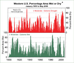
Box 3.6, Figure 1. Percentage of the USA west of the Rocky Mountains (the 11 states west of and including Montana to New Mexico) that was dry (top) or wet (bottom), based on the Palmer Drought Severity Index for classes of moderate to extreme drought or wet. From NOAA, NCDC.
Floods in Europe, Summer 2002
Acatastrophic flood occurred along several central European rivers in August 2002 . The floods resulting from extraordinarily high precipitation were enhanced by the fact that the soils were completely saturated and the river water levels were already high because of previous rain (Rudolf
and Rapp, 2003 [NPR] ;( Ulbrich et al., 2003a, ) b). Hence, it was part of a pattern of weather over an extended period. In the flood, the water levels of the Elbe at Dresden reached a maximum mark of 9.4 m, which is the highest level since records began in 1275 ( (Ulbrich et al., 2003a ) ). Some small villages in the Ore Mountains (on tributaries of the Elbe) were hit by extraordinary flash floods. The river Vltava inundated the city of Prague before contributing to the Elbe flood. A return period of 500 years was estimated for the flood levels at Prague ( (Grollmann and Simon, 2002 ) ). The central European floods were caused by two heavy precipitation episodes. The first, on 6–7 August, was situated mainly over Lower Austria, the southwestern part of the Czech Republic and southeastern Germany. The second took place on 11–13 August 2002 and most severely affected the Ore Mountains and western parts of the Czech Republic. A persistent low-pressure system moved slowly from the Mediterranean Sea to central Europe on a path over or near the eastern Alps and led to large-scale, strong and quasi-stationary frontal lifting of air with very high liquid water content. Additional to this advective rain were convective precipitation processes (showers and thunderstorms) and a significant orographic lifting (mainly over the Ore Mountains). A maximum 24-hour precipitation total of 353 mm was observed at the German station Zinnwald-Georgenfeld, a new record for Germany. The synoptic situation leading to floods is well known to meteorologists of the region. Similar situations led to the summer floods of the River Oder in 1997 and the River Vistula in 2001 ( (Ulbrich et al., 2003b ) ). Average summer precipitation trends in the region are negative but barely significant ( Schönwiese and Rapp, 1997 [NPR] ) and there is no significant trend in flood occurrences of the Elbe within the last 500 years ( Mudelsee et al., 2003 [JoC] ). However, the observed increase in precipitation variability at a majority of German precipitation stations during the last century ( (Trömel and Schönwiese, 2005 ) ) is indicative of an enhancement of the probability of both floods and droughts.
Heat Wave in Europe, Summer 2003
The heat wave that affected many parts of Europe during the course of summer 2003 produced record-breaking temperatures particularly during June and August ( Beniston, 2004 [JoC, SRC] ; Schär et al., 2004 [JoC, ARC] ; see Box 3.6, Figure 2). Absolute maximum temperatures exceeded the record highest temperatures observed in the 1940 s and early 1950 s in many locations in France, Germany, Switzerland, Spain, Italy and the UK, according to the information supplied by national weather agencies ( WMO, 2004 [NPR] ). Gridded instrumental temperatures (from CRUTEM2v for the region 35°N–50°N, 0–20°E) show that the summer was the hottest since comparable records began in 1780 : 3.8°C above the 1961 to 1990 average and 1.4°C hotter than any other summer in this period (the second hottest was 1807 ). Based on early documentary records, Luterbacher et al. 2004 [JoC, ARC] ) estimated that 2003 is very likely to have been the hottest summer since at least 1500 . The 2003 heat wave was associated with a very robust and persistent blocking high-pressure system that may be a manifestation of an exceptional northward extension of the Hadley Cell ( (Black et al., 2004; ) ( Fink et al., 2004 ) ). Already a record month in terms of maximum temperatures, June exhibited high geopotential values that penetrated northwards towards the British Isles, with thegreatest northward extension and longest persistence of record-high temperatures observed in August. An exacerbating factor for the temperature extremes was the lack of precipitation in many parts of western and central Europe, leading to much-reduced soil moisture and surface evaporation and evapotranspiration, and thus to a strong positive feedback effect ( Beniston and Diaz, 2004 [JoC, MoS, SRC] ).
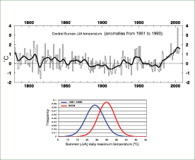
Box 3.6, Figure 2. Long time series of JJA temperature anomalies in Central Europe relative to the 1961 to 1990 mean (top). The smooth curve shows decadal variations (see Appendix 3.A ). In the summer of 2003, the value of 3.8°C far exceeded the next largest anomaly of 2.4°C in 1807, and the highly smoothed Gaussian distribution (bottom) of maximum temperatures (red) compared with normal (blue) at Basel, Switzerland ( Beniston and Diaz, 2004 [JoC, MoS, SRC] ) shows how the whole distribution shifted.
The 2005 Tropical Storm Season in the North Atlantic
The 2005 North Atlantic hurricane season (1 June to 30 November) was the most active on record by several measures, surpassing the very active season of 2004 (e.g., Levinson, 2005 [JoC, SRC] ) and causing an unprecedented level of damage. Even before the peak in the seasonal activity, the seven tropical storms in June and July were the most ever, and hurricane Dennis was the strongest on record in July and the earliest ever fourth-named storm. The record 2005 North Atlantic hurricane season featured the largest number of named storms (28; sustained winds greater than 17 ms–1)and is the only time names have ventured into the Greek alphabet. It had the largest number of hurricanes (15; sustained winds greater than 33 ms–1)recorded, and is the only time there have been four category 5 storms (maximum sustained winds greater than 67 ms–1). These included the most intense Atlantic storm on record (Wilma, with recorded surface pressure in the eye of 882 hPa), the most intense storm in the Gulf of Mexico (Rita, 897 hPa), and Katrina. Tropical storm Vince was the first ever to make landfall in Portugal and Spain. In spite of these metrics, the ACE index, although very high and surpassing the 2004 value( Figure 3.40 ), was not the highest on record, as several storms were quite short lived. Six of the eight most damaging storms on record for the USA occurred from August 2004 to September 2005 (Charlie, Ivan, Francis, Katrina, Rita, Wilma) while another storm in 2005 (Stan) caused severe flooding and mudslides as well as about 2,000 fatalities in central America (Guatemala, El Salvador and southern Mexico).
SSTs in the tropical North Atlantic region critical for hurricanes (10°N to 20°N) were at record-high levels (0.9°C above the 1901 to 1970 normal ) in the extended summer (June to October) of 2005 ( Figure 3.33 ), and these high values were a major reason for the very active hurricane season along with favourable atmospheric conditions (see Box 3.5 ). A substantial component of this warming was the global mean SST increase ( Trenberth and Shea, 2006 [PoC, JoC, SRC] ; see Sections 3.2 and 3.6.6 ).
3.8.4 Evidence for Changes in Extratropical Storms and Extreme Events
3.8.4.1 Extratropical Cyclones
Intense extratropical cyclones are often associated with extreme weather, particularly with severe windstorms. Significant increases in the number or strength of intense extratropical cyclone systems have been documented in a number of studies (e.g., Lambert, 1996 [JoC] ;( Gustafsson, 1997; ) McCabe et al., 2001 [JoC] ; Wang et al., 2006a [JoC, ARC] ) with associated changes in the preferred tracks of storms as described in Section 3.5.3 .As with tropical cyclones, detection of long-term changes in cyclone measures is hampered by incomplete and changing observing systems. Some earlier results have been questioned because of changes in the observation system (e.g., Graham and Diaz, 2001 [JoC] ).
Results from NRA and ERA-40 show that an increase in the number of deep cyclones is apparent over the North Pacific and North Atlantic ( Graham and Diaz, 2001 [JoC] ; Gulev et al., 2001 [JoC, SRC] ), with statistically significant winter increases over both ocean basins ( Simmonds and Keay, 2002 [SRC] ; Wang et al., 2006a [JoC, ARC] Geng and Sugi 2001 [JoC] ) found that cyclone density, deepening rate, central pressure gradient and translation speed have all been increasing in the winter North Atlantic. Caires and Sterl 2005 [JoC, MoS] ) compared global estimates of 100-year return values of wind speed and SWH in ERA-40, with linear bias corrections based on buoy data, for three different 10-year periods. They showed that the differences in the storm tracks can be attributed to decadal variability in the NH, linked to changes in global circulation patterns, most notably to the NAO (see also Section 3.5.6 ).
Using NCEP-2 reanalysis data, Lim and Simmonds 2002 [JoC, SRC] ) showed that for 1979 to 1999, increasing trends in the annual number of explosively developing (deepening by 1 hPa per hour or more) extratropical cyclones are significant in the SH and over the globe (0.56 and 0.78 more systems per year, respectively), while the positive trend did not achieve significance in the NH. Simmonds and Keay 2002 [SRC] ) obtained similar results for the change in the number of cyclones in the decile for deepest cyclones averaged over the North Pacific and over the North Atlantic in winter over the period 1958 to 1997 .
As noted in Sections 3.5.3 and 3.5.7 ,the time-dependent biases in the reanalysis cause uncertainties in the trends reported above. Besides reanalyses, station data may also be used to indicate evidence for changes in extratropical cyclone activity. Instead of direct station wind measurements, which may suffer from a lack of consistency of instrumentation, methodology and exposure, values based on pressure gradients have been derived that are more reliable for discerning long-term changes. Alexandersson et al. 2000 [SRC] ) used station pressure observations for 21 stations over northwestern Europe back to 1881, from which geostrophic winds were calculated using ‘pressure-triangle’ methods. They found a decline of storminess expressed by the 95th and 99th percentiles from high levels during the late 19th century to a minimum around 1960 and then a quite rapid increase to a maximum around 1990, followed again by a decline( Figure 3.41 ). Positive NAO winters are typically associated with more intense and frequent storms (see Section 3.6.4 ). Similar results were obtained by Schmith et al. 1998 [JoC] ) using simpler indices based on pressure tendency. Bärring and von Storch 2004 [JoC] ), using both pressure tendencies and the number of very low pressure values, confirmed these results on the basis of two especially long station series in southern Sweden dating back to about 1800 . Studies of rapid pressure changes at stations indicate an increase in the frequency, duration and intensity of winter cyclone activity over the lower Canadian Arctic and in the number and intensity of severe storms over the southern UK since the 1950 s, but a decrease over southern Canada and Iceland ( Wang et al., 2006b [JoC] ; Alexander et al., 2005 [JoC, SRC] ). Besides a northward shift of the storm track (see 3.5.3), the station pressure data for parts of the North Atlantic region show a modest increase in severe storms in recent decades. However, decadal-scale fluctuations of similar magnitude have occurred earlier in the 19th and 20th centuries.
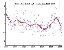
Figure 3.41. Storm index for the British Isles, North Sea and Norwegian Sea, 1881 to 2004 . Blue circles are 95th percentiles and red crosses 99th percentiles of standardised geostrophic winds averaged over 10 sets of triangles of stations. The smoothed curves are a decadal filter (updated from Alexandersson et al., 2000 [SRC] ).
Direct surface wind measurements have, however, been used in a few studies. An analysis of extreme pressure differences and surface winds ( Salinger et al., 2005 [JoC] ) showed a significant increasing trend over the last 40 years in westerly wind extremes over the southern part of New Zealand and the oceans to the south. The trends are consistent with the increased frequency of El Niño events in recent decades, associated with Pacific decadal variability (see Section 3.6.3 ). While the zonal pressure gradient and extreme westerly wind frequency have both increased over southern New Zealand, the frequency of extreme easterly winds has also increased there, suggesting more variability in the circulation generally. However, trends in pressure differences (based on the ERA-40, NRA and station data) are not always consistent with changes in surface windiness (e.g., ( Smits et al., 2005 ) ). Based on observed winds at 10 m height over the Netherlands, ( Smits et al. 2005 ) ) found a decline in strong (greater than about 8 on the Beaufort scale) wind events over the last 40 years. Differences cannot entirely be explained by changes in surface aerodynamic roughness, and they concluded that inhomogeneities in the reanalyses are the cause. However, local differences can be important and intensity and severity of storms may not always be synonymous with local extreme surface winds and gusts.
3.8.4.2 Tornadoes, Hail, Thunderstorms, Dust Storms and Other Severe Local Weather
Evidence for changes in the number or intensity of tornadoes relies entirely on local reports. In the USA, databases for tornado reporting are well established, although changes in procedures for evaluating the intensity of tornadoes introduced significant discontinuities in the record. In particular, the apparent decrease in strong tornadoes in the USA from the early period of the official record ( 1950 s– 1970 s) to the more recent period is, in large part, a result of the way damage from the earlier events was evaluated. ( Trapp et al. 2005 ) ) also questioned the completeness of the tornado record and argued that about 12% of squall-line tornadoes remain unreported. In many European countries, the number of tornado reports has increased considerably over the last decade ( (Snow, 2003 ) ), leading to a much higher estimate of tornado activity ( Dotzek, 2003 [MoS, SRC] Bissolli et al. 2007 [NPR, JoC, SRC, 2007] ) showed that the increase in Germany between 1950 and 2003 mainly concerns weak tornadoes (F0 and F1 on the Fujita scale), thus paralleling the evolution of tornado reports in the USA after 1950 (see, e.g., Dotzek et al., 2005 [JoC, SRC] ) and making it likely that the increase in reports in Europe is at least dominated (if not solely caused) by enhanced detection and reporting efficiency. Doswell et al. 2005 [MoS] ) highlighted the difficulties encountered when trying to find observational evidence for changes in extreme events at local scales connected to severe thunderstorms. In light of the very strong spatial variability of small-scale severe weather phenomena, the density of surface meteorological observing stations is too coarse to measure all such events. Moreover, homogeneity of existing station series is questionable. While remote sensing techniques allow detection of thunderstorms even in remote areas, they do not always uniquely identify severe weather events from these storms. Another approach links severe thunderstorm occurrence to larger-scale environmental conditions in places where the observations of events are fairly good and then consider the changes in the distribution of those environments ( (Brooks et al., 2003; ) Bissolli et al., 2007 [NPR, JoC, SRC, 2007] ).
Although a decreasing trend in dust storms was observed from the mid- 1950 s to the mid- 1990 s in northern China, the number of dust storm days increased from 1997 to 2002 ( (Li and Zhai, 2003; ) ( Zhou and Zhang, 2003 ) ). The decreasing trend appears linked to the reduced cyclone frequency and increasing winter (DJF) temperatures ( Qian et al., 2002 [JoC] ). The recent increase is associated with vegetation degradation and drought, plus increased surface wind speed ( (Wang and Zhai, 2004; ) Zou and Zhai, 2004 [JoC] ).
3.8.5 Summary
Even though the archived data sets are not yet sufficient for determining long-term trends in extremes, there are new findings on observed changes for different types of extremes. The definitions of the phenomena are summarised in Table 3.7 .A summary of the changes in extremes by phenomena, region and time is given in Table 3.8 along with an assessment of the confidence in these changes.
New analyses since the TAR confirm the picture of a gradual reduction of the number of frost days over most of the mid-latitudes in recent decades. In agreement with this warming trend, the number of warm nights increased between 1951 and 2003, cold nights decreased, and trends in the number of cold and warm days are also consistent with warming, but are less marked than at night.
For precipitation, analysis of updated trends and results for regions that were missing at the time of the TAR show increases in heavy events for the majority of observation stations, with some increase in flooding. This result applies both for areas where total precipitation has increased and for areas where total precipitation has even decreased. Increasing trends are also reported for more rare precipitation events, although results for such extremes are available only for a few areas. Mainly because of lack of data, it remains difficult to draw a consistent picture of changes in extreme precipitation for the tropics and subtropics.
Tropical cyclones, hurricanes and typhoons exhibit large variability from year to year and limitations in the quality of data compromise evaluations of trends. Nonetheless, clear evidence exists for increases in category 4 and 5 storms globally since 1970 along with increases in the PDI due to increases in intensity and duration of storms. The 2005 season in the North Atlantic broke many records. The global view of tropical storm activity highlights the important role of ENSO in all basins, and the most active year was 1997, when a very strong El Niño began, suggesting that observed record high SSTs played a key role.
For extratropical cyclones, positive trends in storm frequency and intensity dominate for recent decades in most regional studies performed. Longer records for the northeastern Atlantic suggest that the recent extreme period may be similar in level to that of the late 19th century.
As noted in Section 3.3.4 ,the PDSI shows a large drying trend over NH land areas since the mid- 1950 s and a drying trend in the SH from 1974 to 1998 . Decreases in land precipitation, especially since the early 1980 s are the main cause for the drying trends, although large surface warming during the last two to three decades has also likely contributed to the drying.
Table 3.7. Definition of phenomena used to assess extremes in Table 3.8
| PHENOMENON | Definition |
|---|---|
| Low-temperature days/ nights and frost days | Percentage of days with temperature (maximum for days, minimumfor nights) not exceeding some threshold, either fixed (frost days) or varying regionally (cold days/cold nights), based on the 10th percentile of the daily distribution in the reference period (1961–1990). |
| High-temperature days/nights | See low-temperature days/nights, but now exceeding the 90thpercentile. |
| Cold spells/snaps | Episode of several consecutive low-temperature days/nights. |
| Warm spells (heat waves) | Episode of several consecutive high-temperature days/nights. |
| Cool seasons/warm seasons | Seasonal averages (rather than daily temperatures) exceedingsome threshold. |
| Heavy precipitation events (events that occur every year) | Percentage of days (or daily precipitation amount) with precipitation exceeding some threshold, either fixed or varying regionally, basedon the 95th or 99th percentile of the daily distribution in thereference period (1961–1990). |
| Rare precipitation events (with return periods >~10 yr) | As for heavy precipitation events, but for extremes further into the tail of the distribution. |
| Drought (season/year) | Precipitation deficit; or based on the PDSI (see Box 3.1 ). |
| Tropical cyclones (frequency, intensity, track, peak wind, peak precipitation) | Tropical storm with thresholds crossed in terms of estimated wind speed and organisation. Hurricanes in categories 1 to 5, according tothe Saffir-Simpson scale, are defined as storms with wind speedsof 33 to 42 ms–1,43 to 49 ms–1,50 to 58 ms–1,59 to 69 ms–1,and >70 ms–1,respectively. NOAA’s ACE index is a measure ofthe total seasonal activity that accounts for the collective intensityand duration of tropical storms and hurricanes during agiven tropical cyclone season. |
| Extreme extratropical storms (frequency, intensity, track, surface wind, wave height) | Intense low-pressure systems that occur throughout the mid-latitudes of both hemispheres fueled by temperature gradients and actingto reduce them. |
| Small-scale severe weather phenomena | Extreme events, such as tornadoes, hail, thunderstorms, dust stormsand other severe local weather. |
Table 3.8. Change in extremes for phenomena over the specified region and period, with the level of confidence and section where the phenomenon is discussed in detail.
| PHENOMENON | Change | Region | Period | Confidence | Section |
|---|---|---|---|---|---|
| Low-temperature days/nights and frost days | Decrease, more so for nights than days | Over 70% of global land area | 1951–2003 (last 150 yearsfor Europeand China) | Very likely | 3.8.2.1 |
| High-temperature days/nights | Increase, more so for nights than days | Over 70% of global land area | 1951–2003 | Very likely | 3.8.2.1 |
| Cold spells/snaps (episodes of several days) | Insufficient studies,but daily temperature changes imply a decrease | ||||
| Warm spells (heat waves) (episodes of several days) | Increase: implicit evidence from changes of daily temperatures | Global | 1951–2003 | Likely | FAQ 3.3 |
| Cool seasons/ warm seasons (seasonal averages) | Some new evidence for changes in inter-seasonal variability | Central Europe | 1961–2004 | Likely | 3.8.2.1 |
| Heavy precipitation events (that occur every year) | Increase, generally beyond that expected from changes in the mean (disproportionate) | Many mid-latitude regions (even where reduction in total precipitation) | 1951–2003 | Likely | 3.8.2.2 |
| Rare precipitation events (with return periods > ~10 yr) | Increase | Only a few regions have sufficient data for reliable trends (e.g., UK and USA) | Various since 1893 | Likely (consistent with changes inferred for more robust statistics) | 3.8.2.2 |
| Drought (season/year) | Increase in total area affected | Many land regions of the world | Since 1970s | Likely | 3.3.4 and FAQ 3.3 |
| Tropical cyclones | Trends towards longer lifetimes and greater storm intensity, but no trend in frequency | Tropics | Since 1970s | Likely; more confidence in frequency and intensity | 3.8.3 and FAQ 3.3 |
| Extreme extratropical storms | Net increase in frequency/intensity and poleward shift in track | NH land | Since about 1950 | Likely | 3.8.4 , 3.5, and FAQ 3.3 |
| Small-scale severe weather phenomena | Insufficient studies for assessment |
3.9 Synthesis: Consistency Across Observations
This section briefly compares variability and trends within and across different climate variables to see if a physically consistent picture enhances confidence in the realism of apparent recent observed changes. Therefore, this section looks ahead to the subsequent observational chapters on the cryosphere( Chapter4 )and oceans( Chapter5 ), which focus on changes in those domains. The emphasis here is on inter-relationships. For example, increases in temperature should enhance the moisture-holding capacity of the atmosphere as a whole and changes in temperature and/or precipitation should be consistent with those evident in circulation indices. Variables treated in this chapter are summarised in the executive summary, with some discussion below. The example of increases in temperature that should also reduce snow seasons and sea ice and cause widespread glacier retreat involves cross-chapter variables. The main sections where more detailed information can be found are given in parentheses following each bullet.
- The observed temperature increases are consistent with the observed nearly worldwide reduction in glacier and small ice cap (not including Antarctica and Greenland) mass and extent in the 20th century. Glaciers and ice caps respond not only to temperatures but also to changes in precipitation, and both winter accumulation and summer melting have increased over the last half century in association with temperature increases. In some regions, moderately increased accumulation observed in recent decades is consistent with changes in atmospheric circulation and associated increases in winter precipitation (e.g., southwestern Norway, parts of coastal Alaska, Patagonia, Karakoram, and Fjordland of the South Island of New Zealand), even though enhanced ablation has led to marked declines in mass balances in Alaska and Patagonia. Tropical glacier changes are synchronous with higher-latitude ones and all have shown declines in recent decades; local temperature records all show a slight warming, but not of the magnitude required to explain the rapid reduction in mass of such glaciers (e.g., on Kilimanjaro). Other factors in recent ablation include changes in cloudiness, water vapour, albedo due to snowfall frequency and the associated radiation balance (Sections 3.2.2 , 3.3.3 , 3.4.3 and 4.5 ).
- Snow cover has decreased in many NH regions, particularly in spring, consistent with greater increases in spring as opposed to autumn temperatures in mid-latitude regions, and more precipitation falling as rain instead of snow. These changes are consistent with changes in permafrost: temperatures of the permafrost in the Arctic and subarctic have increased by up to 3°C since the 1980s with permafrost warming also observed on the Tibetan Plateau and in the European mountain permafrost regions. Active layer thickness has increased and seasonally frozen ground depth has decreased over the Eurasian continent (Sections 3.2.2 , 3.3.2 , 4.2 and 4.8 ).
- Sea ice extents have decreased in the Arctic, particularly in spring and summer, and patterns of the changes are consistent with regions showing a temperature increase, although changes in winds are also a major factor. Sea ice extents were at record low values in 2005, which was also the warmest year since records began in 1850 for the Arctic north of 65°N. There have also been decreases in sea ice thickness. In contrast to the Arctic, antarctic sea ice does not exhibit any significant trend since the end of the 1970s, which is consistent with the lack of trend in surface temperature south of 65°S over that period. However, along the Antarctic Peninsula, where significant warming has occurred, progressive breakup of ice shelves has occurred beginning in the late 1980s, culminating in the breakup of the Larsen-B ice shelf in 2002. Decreases are found in the length of the freeze season of river and lake ice (Sections 3.2.2 , 3.6.5 , 4.3 and 4.4 ).
- Radiation changes at the top of the atmosphere from the 1980s to 1990s, possibly ENSO-related in part, appear to be associated with reductions in tropical cloud cover, and are linked to changes in the energy budget at the surface and in observed ocean heat content in a consistent way (Sections 3.4.3 , 3.4.4 , 3.6.2 and 5.2.2 ).
- Reported decreases in solar radiation from 1970 to 1990 at the surface have an urban bias. Although records are sparse, pan evaporation is estimated to have decreased in many places due to decreases in surface radiation associated with increases in clouds, changes in cloud properties and/or increases in air pollution (aerosol), especially from 1970 to 1990. There is evidence to suggest that the solar radiation decrease has reversed in recent years (Sections 2.4.5 ,2.4.6, 3.3.3 , 3.4.4 , 7.2 and 7.5 ).
- Droughts have increased in spatial extent in various parts of the world. The regions where they have occurred seem to be determined largely by changes in SSTs, especially in the tropics, through changes in the atmospheric circulation and precipitation. Inferred enhanced evapotranspiration and drying associated with warming are additional factors in drought increases, but decreased precipitation is the dominant factor. In the western USA, diminishing snowpack and subsequent summer soil moisture reductions have also been a factor. In Australia and Europe, direct links to warming have been inferred through the extreme nature of high temperatures and heat waves accompanying drought (Sections 3.3.4 and 4.2 , FAQ 3.2 and Box 3.6 ).
- Changes in the freshwater balance of the Atlantic Ocean over the past four decades have been pronounced, as freshening has occurred in the North Atlantic and south of 25°S, while salinity has increased in the tropics and subtropics, especially in the upper 500 m. The implication is that there have been increases in moisture transport by the atmosphere from the subtropics to higher latitudes, in association with changes in atmospheric circulation, including the NAO, thereby producing the observed increases in precipitation over the northern oceans and adjacent land areas (Sections 3.3.2 , 3.6.4 , 5.3.2 and 5.5.3 ).
- Sea level likely rose 1.7 ± 0.5 mm yr–1 during the 20th century, but the rate increased to 3.1 ± 0.7 mm yr–1 from 1993 through 2003, when confidence increases from global altimetry measurements. Increases in ocean heat content and associated ocean expansion are estimated to have contributed 0.4 ± 0.1 mm yr–1 from 1961 to 2003, increasing to an estimated value of 1.6 ± 0.5 mm yr–1 for 1993 to 2003. In the same interval, glacier and land ice melt has increased ocean mass by approximately 1.2 ± 0.4 mm yr–1.Changes in land water storage are uncertain but may have reduced water in the ocean. The near balance for 1993 to 2003 gives increased confidence that the observed sea level rise is a strong indicator of warming, and an integrator of the cumulative energy imbalance at the top of atmosphere (Sections 4.5 , 4.6 , 4.8 , 5.2 and 5.5 ).
In summary, global mean temperatures have increased since the 19th century, especially since the mid- 1970 s. Temperatures have increased nearly everywhere over land, and SSTs and marine air temperatures have also increased, reinforcing the evidence from land. However, temperatures have increased neither monotonically nor in a spatially uniform manner, especially over shorter time intervals. The atmospheric circulation has also changed: in particular, increasing zonal flow is observed in most seasons in both hemispheres, and the mid- to high-latitude annular modes strengthened until the mid- 1990 s in the NH and up until the present in the SH. In the NH, this brought milder maritime air into Europe and much of high-latitude Asia from the North Atlantic in winter, enhancing warming there. In the SH, where the ozone hole has played a role, it has resulted in cooling over 1971 to 2000 for parts of the interior of Antarctica but large warming in the Antarctic Peninsula region and Patagonia. Temperatures generally have risen more than average where flow has become more poleward, and less than average or even cooled where flow has become more equatorward, reflecting the PDO and other patterns of variability.
Over land, a strong negative correlation is observed between precipitation and surface temperature in summer and at low latitudes throughout the year, and areas that have become wetter, such as the eastern USA and Argentina, have not warmed as much as other land areas (see especially FAQs 3.2 and 3.3 ). Increased precipitation is associated with increases in cloud and surface wetness, and thus increased evapotranspiration. The inferred increased evapotranspiration and reduced temperature increase is physically consistent with enhanced latent vs. sensible heat fluxes from the surface in wetter conditions.
Consistent with the expectations noted above for a warmer climate, surface specific humidity has generally increased after 1976 in close association with higher temperatures over both land and ocean. Total column water vapour has increased over the global oceans by 1.2 ± 0.3% per decade from 1988 to 2004, consistent in patterns and amount with changes in SST and a fairly constant relative humidity. Upper-tropospheric water vapour has also increased in ways such that relative humidity remains about constant, providing a major positive feedback to radiative forcing. In turn, widespread observed increases in the fraction of heavy precipitation events are consistent with the increased water vapour amounts.
The three main ocean basins are unique and contain very different wind systems, SST patterns and currents, leading to vastly different variability associated, for instance, with ENSO in the Pacific, and the THC in the Atlantic. Consequently, the oceans have not warmed uniformly, especially at depth. SSTs in the tropics have warmed at different rates and help drive, through coupling with tropical convection and winds, teleconnections around the world. This has changed the atmospheric circulation through ENSO, the PDO, the AMO, monsoons and the Hadley and Walker Circulations. Changes in precipitation and storm tracks are not as well documented but clearly respond to these changes on interannual and decadal time scales. When precipitation increases over the ocean, as it has in recent years in the tropics, it decreases over land, although it has increased over land at higher latitudes. Droughts have increased over many tropical and mid-latitude land areas, in part because of decreased precipitation over land since the 1970 s but also from increased evapotranspiration arising from increased atmospheric demand associated with warming.
Changes in the cryosphere( Chapter4 ), ocean and land strongly support the view that the world is warming, through observed decreases in snow cover and sea ice, thinner sea ice, shorter freezing seasons of lake and river ice, glacier melt, decreases in permafrost extent, increases in soil temperatures and borehole temperature profiles (see Section 6.6 ), and sea level rise( Section 5.5 ).
Acknowledgments
The authors gratefully acknowledge the valuable assistance of Sara Veasey (NCDC, Asheville) and Lisa Butler (NCAR, Boulder) in the development of diagrams and text formatting.
Appendix 3.B: Techniques, Error Estimation and Measurement Systems: See Supplementary Material
This material is included in the supplementary material. Please note that the many references that are cited only in Appendix 3.B have not been included in the list above, but are just as valuable in formulating the report.
Appendix 3.A:Low-Pass Filters and Linear Trends
The time series used in this report have undergone diverse quality controls that have, for example, led to removal of outliers, thereby building in some smoothing. In order to highlight decadal and longer time-scale variations and trends, it is often desirable to apply some kind of low-pass filter to the monthly, seasonal or annual data. In the literature cited for the many indices used in this chapter, a wide variety of schemes was employed. In this chapter, the same filter was used wherever it was reasonable to do so. The desirable characteristics of such filters are 1) they should be easily understood and transparent; 2) they should avoid introducing spurious effects such as ripples and ringing ( (Duchon, 1979 ) ); 3) they should remove the high frequencies; and 4) they should involve as few weighting coefficients as possible, in order to minimise end effects. The classic low-pass filters widely used have been the binomial set of coefficients that remove 2∆t fluctuations, where ∆t is the sampling interval. However, combinations of binomial filters are usually more efficient, and those have been chosen for use here, for their simplicity and ease of use. Mann 2004 [PoC, JoC] ) discusses smoothing time series and especially how to treat the ends. This chapter uses the ‘minimum slope’ constraint at the beginning and end of all time series, which effectively reflects the time series about the boundary. If there is a trend, it will be conservative in the sense that this method will underestimate the anomalies at the end.
The first filter (e.g., Figure 3.5 )is used in situations where only the smoothed series is shown, and it is designed to remove interannual fluctuations and those on El Niño time scales. It has 5 weights 1/12 [1-3-4-3-1] and its response function (ratio of amplitude after to before) is 0.0 at 2 and 3∆t, 0.5 at 6∆t, 0.69 at 8∆t, 0.79 at 10∆t, 0.91 at 16∆t, and 1 for zero frequency, so for yearly data (∆t = 1) the half-amplitude point is for a 6-year period, and the half-power point is near 8.4 years.
The second filter used in conjunction with annual values (∆t =1) or for comparisons of multiple curves (e.g., Figure 3.8 )is designed to remove fluctuations on less than decadal time scales. It has 13 weights 1/576 [1-6-19-42-71-96-106-96-71-42-19-6-1]. Its response function is 0.0 at 2, 3 and 4∆t, 0.06 at 6∆t, 0.24 at 8∆t, 0.41 at 10∆t, 0.54 at 12∆t, 0.71 at 16∆t, 0.81 at 20∆t, and 1 for zero frequency, so for yearly data the half-amplitude point is about a 12-year period, and the half-power point is 16 years. This filter has a very similar response function to the 21-term binomial filter used in the TAR.
Another low-pass filter, widely used and easily understood, is to fit a linear trend to the time series although there is generally no physical reason why trends should be linear, especially over long periods. The overall change in the time series is often inferred from the linear trend over the given time period, but can be quite misleading. Such measures are typically not stable and are sensitive to beginning and end points, so that adding or subtracting a few points can result in marked differences in the estimated trend. Furthermore, as the climate system exhibits highly nonlinear behaviour, alternative perspectives of overall change are provided by comparing low-pass-filtered values (see above) near the beginning and end of the major series.
The linear trends are estimated by Restricted Maximum Likelihood regression (REML, Diggle et al., 1999 [NPR] ), and the estimates of statistical significance assume that the terms have serially uncorrelated errors and that the residuals have an AR1 structure. Brohan et al. 2006 [JoC, MoS] and Rayner et al. 2006 [JoC] ) provide annual uncertainties, incorporating effects of measurement and sampling error and uncertainties regarding biases due to urbanisation and earlier methods of measuring SST. These are taken into account, although ignoring their serial correlation. The error bars on the trends, shown as 5 to 95% ranges, are wider and more realistic than those provided by the standard ordinary least squares technique. If, for example, a century-long series has multi-decadal variability as well as a trend, the deviations from the fitted linear trend will be autocorrelated. This will cause the REML technique to widen the error bars, reflecting the greater difficulty in distinguishing a trend when it is superimposed on other long-term variations and the sensitivity of estimated trends to the period of analysis in such circumstances. Clearly, however, even the REML technique cannot widen its error estimates to take account of variations outside the sample period of record. Robust methods for the estimation of linear and nonlinear trends in the presence of episodic components became available recently ( Grieser et al., 2002 [SRC] ).
As some components of the climate system respond slowly to change, the climate system naturally contains persistence. Hence, the statistical significances of REML AR1-based linear trends could be overestimated ( Zheng and Basher, 1999 [JoC, MoS] ; Cohn and Lins, 2005 [JoC] ). Nevertheless, the results depend on the statistical model used, and more complex models are not as transparent and often lack physical realism. Indeed, long-term persistence models ( Cohn and Lins, 2005 [JoC] ) have not been shown to provide a better fit to the data than simpler models.
References
Abakumova, G.M., et al., 1996: Evaluation of long-term changes in radiation, cloudiness, and surface temperature on the territory of the former Soviet Union. J. Clim., 9,1319–1327. [JoC]
Adler, R.F., et al., 2001: Intercomparison of global precipitation products: The Third Precipitation Intercomparison Project (PIP-3). Bull. Am. Meteorol. Soc., 82,1377–1396. [JoC, SRC]
Adler, R.F., et al., 2003: The version 2 Global Precipitation Climatology Project (GPCP) monthly precipitation analysis (1979–present). J. Hydrometeorol., 4,1147–1167. [JoC, SRC]
Agudelo, P.A., and J.A. Curry, 2004: Analysis of spatial distribution in tropospheric temperature trends. Geophys. Res. Lett., 31,L22207, doi:10.1029/2004GL02818. [JoC]
Aguilar, E., et al., 2005: Changes in precipitation and temperature extremes in Central America and northern South America, 1961–2003. J. Geophys. Res., 110,D23107, doi:10.1029/2005JD006119. [JoC]
Aiyyer, A.R., and C. Thorncroft, 2006: Climatology of vertical wind shear over the tropical Atlantic. J. Clim., 19,2969−2983. [JoC, SRC]
Aksoy, B., 1997: Variations and trends in global solar radiation for Turkey. Theor. Appl. Climatol., 58,71–77. Clean
Alexander, L.V., S.F.B. Tett, and T. Jónsson, 2005: Recent observed changes in severe storms over the United Kingdom and Iceland. Geophys. Res. Lett., 32,L13704, doi:10.1029/2005GL022371. [JoC, SRC]
Alexander, L.V., et al., 2006: Global observed changes in daily climate extremes of temperature and precipitation. J. Geophys. Res., 111,D05109, doi:10.1029/2005JD006290. [JoC, SRC]
Alexandersson, H., et al., 1998: Long-term variations of the storm climate over NW Europe. Global Atmos. Ocean System, 6,97–120. [SRC]
Alexandersson, H., et al., 2000: Trends of storms in NW Europe derived from an updated pressure data set. Clim. Res., 14,71–73. [SRC]
Allan, J., and P. Komar, 2000: Are ocean wave heights increasing in the eastern North Pacific? Eos, 81,561–567. [JoC]
Allan, R.J., and T. Ansell, 2006: A new globally complete monthly historical gridded mean sea level pressure data set (HadSLP2); 1850–2003. J. Clim., 19,5816–5842. [JoC, SRC]
Allan, R.P., and A. Slingo, 2002: Can current climate model forcings explain the spatial and temporal signatures of decadal OLR variations? Geophys. Res. Lett., 29,1141, doi:10.1029/2001GL014620. [JoC, MoS]
Allan, R.P., A. Slingo, and V. Ramaswamy, 2002: Analysis of moisture variability in the European Centre for Medium-Range Weather Forecasts 15-year reanalysis over tropical oceans. J. Geophys. Res., 107,doi:10.1029/2001JD001132. [NPR, JoC, MoS, ARC]
Allan, R.P., M.A. Ringer, and A. Slingo, 2003: Evaluation of moisture in the Hadley Centre Climate Model using simulations of HIRS water vapour channel radiances. Q. J. R. Meteorol. Soc., 128,1–18. [JoC, MoS]
Allan, R.P., et al., 2001: Is there an equatorial Indian Ocean dipole, and is it independent of the El Niño Southern Oscillation? CLIVAR Exchanges, 21,1–3. Clean
Allan, R.P., et al., 2004: Simulation of the Earth’s radiation budget by the European Centre for Medium-Range Weather Forecasts 40-year reanalysis (ERA40). J. Geophys. Res., 109,D18107, doi:10.1029/2004JD004816. [JoC, MoS]
Allen, M.R., and W.J. Ingram, 2002: Constraints on future changes in climate and the hydrological cycle. Nature, 419,2224–2232. [JoC, MoS, ARC]
Alley, W.M., 1984: The Palmer Drought Severity Index: limitation and assumptions. J. Clim. Appl. Meteorol., 23,1100–1109. Clean
Alpert, P., et al., 2002: The paradoxical increase of Mediterranean extreme daily rainfall in spite of decrease in total values. Geophys. Res. Lett., 29(11), doi:10.1029/2001GL013554. [JoC]
Alpert, P., et al., 2005: Global dimming or local dimming?: Effect of urbanization on sunlight availability. Geophys. Res. Lett., 32,L17802, doi:10.1029/2005GL023320. [JoC]
Ambaum, M.H.P., B.J. Hoskins, and D.B. Stephenson, 2001: Arctic Oscillation or North Atlantic Oscillation? J. Clim., 14,3495–3507. [JoC, SRC]
Ambaum, M.H.P., B.J. Hoskins, and D.B. Stephenson, 2002: Corrigendum: Arctic Oscillation or North Atlantic Oscillation? J. Clim., 15,553. [JoC, SRC]
Andrea, F., et al., 1998: Northern Hemisphere atmospheric blocking as simulated by 15 atmospheric general circulation models in the period 1979–1988. Clim. Dyn., 14,385–407. [JoC, MoS]
Andreae, M.O., et al., 2004: Smoking rain clouds over the Amazon. Science, 303,1337–1342. [JoC]
Andrews, D.G., J.R. Holton, and C.B. Leovy, 1987: Middle Atmosphere Dynamics.Academic Press, San Diego, CA, 489 pp. [NPR]
Angell, J.K., 2003: Effect of exclusion of anomalous tropical stations on temperature trends from a 63-station radiosonde network, and comparison with other analyses. J. Clim., 16,2288–2295. [JoC]
Angell, J.K., 2006: Changes in the 300 mb north circumpolar vortex, 1963–2001. J. Clim., 19,2984–2994. [JoC]
Aoki, S., 2002: Coherent sea level response to the Antarctic Oscillation. Geophys. Res. Lett., 29,1950, doi:10.1029/2002GL15733. [JoC]
Ashok, K., Z. Guan, and T. Yamagata, 2001: Impact of the Indian Ocean Dipole on the decadal relationship between the Indian monsoon rainfall and ENSO. Geophys. Res. Lett., 28,4499–4502. [JoC]
Assell, R., K. Cronk, and D. Norton, 2003: Recent trends in Laurentian Great Lakes ice cover. Clim. Change, 57,185–204. [JoC]
Auer, I., et al., 2007: HISTALP -- Historical Instrumental Climatological Surface Time Series of the Greater Alpine Region. Int. J. Climatol., 27,17-46. [JoC, ARC, 2007]
Baldwin, M.P., 2001: Annular modes in global daily surface pressure. Geophys. Res. Lett., 28,4115–4118. [JoC, SRC]
Baldwin, M.P., and T. Dunkerton, 1999: Downward propagation of the Arctic Oscillation from the stratosphere to the troposphere. J. Geophys. Res., 104,30937–30946. [JoC, SRC]
Baldwin, M.P., and T.J. Dunkerton, 2001: Stratospheric harbingers of anomalous weather regimes. Science, 244,581–584. [JoC, SRC]
Baldwin, M.P., et al., 2003: Stratospheric memory and extended-range weather forecasts. Science, 301,636–640. [JoC, MoS, SRC]
Balling, R.C. Jr., and S. Brazel, 1987: Recent changes in Phoenix summertime diurnal precipitation patterns. Theor. Appl. Climatol., 38,50–54. Clean
Balling, R.C. Jr., et al., 1998: Impacts of land degradation on historical temperature records from the Sonoran Desert. Clim. Change, 40,669–681. [JoC]
Barlow, M., H. Cullen, and B. Lyon, 2002: Drought in central and southwest Asia: La Niña, the warm pool, and Indian Ocean precipitation. J. Clim., 15,697–700. [JoC]
Barnett, T.P., et al., 1999: Interdecadal interactions between the tropics and midlatitudes in the Pacific basin. Geophys. Res. Lett., 26,615–618. [JoC]
Barnston, A.G., and R.E. Livezey, 1987: Classification, seasonality and persistence of low frequency atmospheric circulation patterns. Mon. Weather Rev., 115,1083–1126. [JoC]
Bärring, L., and H. von Storch, 2004: Scandinavian storminess since about 1800. Geophys. Res. Lett., 31,L20202, doi:10.1029/2004GL020441. [JoC]
Barriopedro, D., et al., 2006: A climatology of Northern Hemisphere blocking. J. Clim., 19,1042–1063. [JoC]
Barros, V.R., M.E. Castañeda, and M.E. Doyle, 2000a: Recent precipitation trends in southern South America east of the Andes: An indication of climatic variability. In: Southern Hemisphere Paleo- and Neoclimates. Key Sites, Methods, Data and Models [Smolka, P.P., and W. Volkheimer (eds.)]. Springer Verlag, Berlin, pp. 187–206. [NPR, MoS]
Barros, V.R., et al., 2000b: Influence of the South Atlantic Convergence Zone and South Atlantic sea surface temperature on interannual summer rainfall variability in southeastern South America. Theor. Appl. Climatol., 67,123–133. Clean
Barros, V.R., et al., 2002: Climate variability over South America and the South America monsoon: A review. Meteorologica, 27,33–57. Clean
Barros, V.R., et al., 2004: The major discharge events in the Paraguay River: magnitudes, source regions and climate forcings. J. Hydrometeorol., 6,1161–1170. [JoC, MoS]
Basher, R.E., and X. Zheng, 1995: Tropical cyclones in the southwest Pacific: Spatial patterns and relationships to Southern Oscillation and sea surface temperature. J. Clim., 8,1249–1260. [JoC]
Bates, J.J., and D.L. Jackson, 2001: Trends in upper-tropospheric humidity.Geophys. Res. Lett., 28,1695–1698. Clean
Beck, C., J. Grieser, and B. Rudolf, 2005: A new monthly precipitation climatology for the global land areas for the period 1951 to 2000. Climate Status Report, 2004.German Meteorological Service, pp. 181–190, http://www.dwd.de/de/FundE/Klima/KLIS/prod/KSB/ksb04/28_precipitation.pdf [NPR, SRC]
Bengtsson, L., S. Hagemann, and K.L. Hodges, 2004: Can climate trends be calculated from reanalysis data? J. Geophys. Res., 109,D11111, doi:10.1029/2004JD004536. [JoC, ARC]
Beniston, M., 2004: The 2003 heat wave in Europe. A shape of things to come? Geophys. Res. Lett., 31,L02022, doi:10.1029/2003GL018857. [JoC, SRC]
Beniston, M., and H.F. Diaz, 2004: The 2003 heat wave as an example of summers in a greenhouse climate? Observations and climate model simulations for Basel, Switzerland. Global Planet. Change, 44,73–81. [JoC, MoS, SRC]
Beniston, M., and D.B. Stephenson, 2004: Extreme climatic events and their evolution under changing climatic conditions. Global Planet. Change, 44,1–9. [JoC, SRC]
Berger, C.L., et al., 2002: A climatology of northwest Missouri snowfall events: Long-term trends and interannual variability. Phys. Geogr., 23,427−448. Clean
Berri, G.S., M.A. Ghietto, and N.O. García, 2002: The influence of ENSO in the flows of the Upper Paraná River of South America over the past 100 years. J. Hydrometeorol., 3,57–65. [JoC]
Betts, A.K., J.H. Ball, and P. Viterbo, 2003: Evaluation of the ERA-40 surface water budget and surface temperature for the Mackenzie River Basin. J. Hydrometeorol., 4,1194–1211. [JoC]
Biondi, F., A. Gershunov, and D.R. Cayan, 2001: North Pacific decadal climate variability since AD 1661. J. Clim., 14,5–10. [JoC, SRC]
Bischoff, S.A., et al., 2000: Climate variability and Uruguay River flows. Water International, 25,446–456. Clean
Bissolli, P., J. Grieser, N. Dotzek, and M. Welsch, 2007: Tornadoes in Germany 1950-2003 and their relation to particular weather conditions. Global Planet. Change, 46,doi:10.1016/j.gloplacha.2006.11.007 [NPR, JoC, SRC, 2007]
Black, E.M., et al., 2004: Factors contributing to the summer 2003 European heatwave. Weather, 59,217–223. Clean
Bojariu, R., and L. Gimeno, 2003: The influence of snow cover fluctuations on multiannual NAO persistence. Geophys. Res. Lett., 30,1156, doi:10.1029/2002GL015651. [JoC]
Bonan, G.B., 2001: Observational evidence for reduction of daily maximum temperature by croplands in the midwest United States. J. Clim., 14,2430–2442. [JoC, ARC]
Bonnazola, M., and P.H. Haynes, 2004: A trajectory-based study of the tropical tropopause region. J. Geophys. Res., 109,D020112, doi:10.1029/2003JD004356. [JoC]
Bornstein, R., and Q. Lin, 2000: Urban heat islands and summertime convective thunderstorms in Atlanta: three cases studies. Atmos. Environ., 34,507–516. Clean
Bottomley, M., et al., 1990: Global Ocean Surface Temperature Atlas “GOSTA”.HMSO, London, 20 pp.+iv, 313 plates. [NPR]
Bove, M.C., et al., 1998: Effect of El Niño on U.S. landfalling hurricanes, revisited. Bull. Am. Meteorol. Soc., 79,2477–2482. [JoC]
Branstator, G., 2002: Circum-global teleconnections, the jetstream waveguide, and the North Atlantic Oscillation. J. Clim., 15,1893–1910. [JoC]
Brest, C.L., W.B. Rossow, and M. Roiter, 1997: Update of radiance calibrations for ISCCP. J. Atmos. Ocean Technol., 14,1091–1109. Clean
Brohan, P., et al., 2006: Uncertainty estimates in regional and global observed temperature changes: A new dataset from 1850. J. Geophys. Res., 111,D12106, doi:10.1029/2005JD006548. [JoC, MoS]
Bromirski, P.D., R.E. Flick, and D.R. Cayan, 2003: Storminess variability along the California coast: 1858–2000. J. Clim., 16,982–993. [JoC, SRC]
Bromwich, D.H., and R.L. Fogt, 2004: Strong trends in the skill of the ERA-40 and NCEP–NCAR reanalyses in the high and middle latitudes of the Southern Hemisphere, 1958–2001.J. Clim., 17,4603–4619. [SRC]
Brönnimann, S., et al., 2004: Extreme climate of the global troposphere and stratosphere in 1940–42 related to El Niño. Nature, 431,doi:10.1038/nature02982. [NPR, JoC]
Brooks, H.E., J.W. Lee, and J.P. Craven, 2003: The spatial distribution of severe thunderstorm and tornado environments from global reanalysis data. Atmos. Res., 67–68,73–94. Clean
Brunet, M., et al., 2006: The development of a new dataset of Spanish daily adjusted temperature series (SDATS) (1850-2003). Int. J. Climatol., 26,1777–1802. [JoC]
Brunetti, M., et al., 2004: Changes in daily precipitation frequency and distribution in Italy over the last 120 years. J. Geophys. Res., 109,D05102, doi:10.1029/2003JD004296. [JoC]
Brutsaert, W., and M.B. Parlange, 1998: Hydrologic cycle explains the evaporation paradox. Nature, 396,30. [JoC]
Burian, S.J., and J.M. Shepherd, 2005: Effects of urbanization on the diurnal rainfall pattern in Houston. Hydrological Processes: Special Issue on Rainfall and Hydrological Processes, 19,1089–1103. [NPR, SRC]
Burnett, A.W., et al., 2003: Increasing Great Lake-effect snowfall during the Twentieth Century: A regional response to global warming? J. Clim., 16,3535–3541. [JoC]
Caesar, J., L. Alexander, and R. Vose, 2006: Large-scale changes in observed daily maximum and minimum temperatures: Creation and analysis of a new gridded data set. J. Geophys. Res., 111,D05101, doi:10.1029/2005JD006280. [JoC, SRC]
Cai, W., and P.G. Baines, 2001: Forcing of the Antarctic Circumpolar Wave by El Niño-Southern Oscillation teleconnections. J. Geophys. Res., 106,9019–9038. [JoC, MoS, ARC]
Cai, W., P.H. Whetton, and D.J. Karoly, 2003: The response of the Antarctic Oscillation to increasing and stabilized atmospheric CO2. J. Clim., 16,1525–1538. [JoC, ARC]
Caires, S., and A. Sterl, 2005: 100-year return value estimates for wind speed and significant wave height from the ERA-40 data. J. Clim., 18,1032–1048. [JoC, MoS]
Camargo, S.J., and A.H. Sobel, 2004: Western North Pacific Tropical Cyclone Intensity and ENSO.Technical Report No. 04-03, International Research Institute for Climate Prediction, Palisades, NY, 25 pp. [NPR, MoS]
Camilloni, I.A., and V.R. Barros, 2000: The Paraná River response to El Niño 1982–83 and 1997–98 events. J. Hydrometeorol., 1,412–430. [JoC, SRC]
Camilloni, I.A., and V.R. Barros, 2003: Extreme discharge events in the Paraná River and their climate forcing. J. Hydrol., 278,94–106. [MoS, SRC]
Cardone, V.J., J.G. Greenwood, and M.A. Cane, 1990: On trends in historical marine wind data. J. Clim., 3,113–127. [JoC]
Carril, A.F., and A. Navarra, 2001: Low-frequency variability of the Antarctic Circumpolar Wave. Geophys. Res. Lett., 28,4623–4626. [JoC]
Carter, D.J.T., 1999: Variability and trends in the wave climate of the North Atlantic: a review. In: Proceedings of the 9th International Offshore and Polar Engineering Conference, Brest, France, vol. III. International Society of Offshore and Polar Engineers, Golden, CO, pp. 12–18. [NPR]
Cassou, C., and L. Terray, 2001: Dual influence of Atlantic and Pacific SST anomalies on the North Atlantic/Europe winter climate. Geophys. Res. Lett., 28,3195–3198. [JoC, SRC]
Cassou, C., et al., 2004: North Atlantic winter climate regimes: spatial asymmetry, stationarity with time and oceanic forcing. J. Clim., 17,1055–1068. [JoC, MoS, SRC]
Cayan, D.R., et al., 2001: Changes in the onset of spring in the western United States. Bull. Am. Meteorol. Soc., 82,399–415. [JoC, SRC]
Cess, R.D., and P.M. Udelhofen, 2003: Climate change during 1985–1999: Cloud interactions determined from satellite measurements. Geophys. Res. Lett., 30,1019, doi:10.1029/2002GL016128. [JoC]
Chagnon, F.J.F., and R. L. Bras, 2005: Contemporary climate change in the Amazon. Geophys. Res. Lett., 32,L13703, doi:10.1029/2005GL022722. [JoC]
Chan, J.C.L., 2006: Comment on “Changes in tropical cyclone number, duration, and intensity in a warming environment”. Science, 311,1713. [JoC]
Chan, J.C.L., and K.S. Liu, 2004: Global warming and Western North Pacific typhoon activity from an observational perspective. J. Clim., 17,4590–4602. [JoC]
Chang, C.P., Y. Zhang, and T. Li, 1999: Interannual and interdecadal variations of the East Asian summer monsoon and tropical Pacific SSTs. Pt I: Roles of the subtropical ridge. J. Clim., 13,4310–4325. [JoC]
Chang, E.K.M., 2003: Midwinter suppression of the Pacific storm track activity as seen in aircraft observations.J. Atmos. Sci., 60,1345–1358. [SRC]
Chang, E.K.M., and Y. Fu, 2002: Interdecadal variations in Northern Hemisphere winter storm track intensity. J. Clim., 15,642–658. [JoC, SRC]
Chang, E.K.M., and Y. Fu, 2003: Using mean flow change as a proxy to infer interdecadal storm track variability. J. Clim., 16,2178–2196. [JoC, SRC]
Changnon, D., M. Sandstrom, and C. Schaffer, 2003: Relating changes in agricultural practices to increasing dew points in extreme Chicago heat waves. Clim. Res., 24,243–254. Clean
Changnon, S.A., and N.E. Westcott, 2002: Heavy rainstorms in Chicago: Increasing frequency, altered impacts, and future implications. J. Am. Water Res. Assoc., 38,1467–1475. [MoS]
Changnon, S.A., et al., 1981: METROMEX:A Review and Summary.Meteorological Monograph 18, American Meteorological Society, Boston, MA, 81 pp. [NPR]
Chase, T.N., J.A. Knaff, R.A. Pielke Sr., and E. Kalnay, 2003: Changes in global monsoon circulation since 1950. Natural Hazards, 29,229–254. Clean
Chattopadhyay, N., and M. Hulme, 1997: Evaporation and potential evapotranspiration in India under conditions of recent and future climate change. Agric. For. Meteorol., 87,55–73. [MoS]
Chelliah, M., and G.D. Bell, 2004: Tropical multidecadal and interannual climate variability in the NCEP–NCAR Reanalysis. J. Clim., 17,1777–1803. [JoC]
Chelton, D.B., and F.J. Wentz, 2005: Global microwave satellite observations of sea surface temperature for numerical weather prediction and climate research. Bull. Am. Meteorol. Soc., 86,1097–1115. [JoC, MoS]
Chen, M., P. Xie, and J.E. Janowiak, 2002: Global land precipitation: a 50-yr monthly analysis based on gauge observations. J. Hydrometeorol., 3,249–266. [JoC]
Chen, T.-C., et al., 2004: Variation of the East Asian summer monsoon rainfall. J. Clim., 17,744–762. [JoC]
Christy, J.R., and W.B. Norris, 2004: What may we conclude about tropospheric temperature trends? Geophys. Res. Lett., 31,L0621, doi:10.1029/2003GL019361. [JoC, SRC]
Christy, J. R., and R.W. Spencer, 2005: Correcting temperature data sets.Science, 310,972. [NPR, SRC]
Christy, J.R., R.W. Spencer, and W.D. Braswell, 2000: MSU tropospheric temperatures: Dataset construction and radiosonde comparisons. J. Atmos. Ocean. Technol., 17,1153–1170. [SRC]
Christy, J.R., et al., 2001: Differential trends in tropical sea surface and atmospheric temperature since 1979. Geophys. Res. Lett., 28,183–186. [JoC, SRC]
Christy, J.R., et al., 2003: Error estimates of version 5.0 of MSU/AMSU bulk atmospheric temperatures. J. Atmos. Ocean. Technol., 20,613–629. [MoS, SRC]
Clark, C.O., P.J. Webster, and J.E. Cole, 2003: Interdecadal variability of the relationship between the Indian Ocean zonal mode and east African coastal rainfall anomalies. J. Clim., 16,548–554. [JoC, ARC]
Cluis, D., and C. Laberge, 2001: Climate change and trend detection in selected rivers within the Asia-Pacific region. Water International, 26,411–424. Clean
Cohen, S., B. Liepert, and G. Stanhill, 2004: Global dimming comes of age. Eos, 85,362. [JoC, SRC]
Cohn, T., and H.J. Lins, 2005: Nature’s style: Naturally trendy. Geophys. Res. Lett., 32,L23402, doi:10.1029/2005GL024476. [JoC]
Compo, G.P., and P.D. Sardeshmukh, 2004: Storm track predictability on seasonal and decadal scales. J. Clim., 17,3701–3720. [JoC, MoS]
Connolley, W.M., 2003: Long-term variation of the Antarctic Circumpolar Wave. J. Geophys. Res., 108,8076, doi:10.1029/2000JC000380. [JoC]
Considine, D.B., et al., 2001: An interactive model study of the influence of the Mount Pinatubo aerosol on stratospheric methane and water trends. J. Geophys. Res., 106,27711–27728. [JoC, MoS]
Cook, E.R., R.D. D’Arrigo, and M.E. Mann, 2002: A well-verified, multiproxy reconstruction of the winter North Atlantic Oscillation index since A.D. 1400. J. Clim., 15,1754–1764. [PoC, JoC, ARC]
Cook, E.R., et al., 1999: Drought reconstructions for the continental United States. J. Clim., 12,1145–1162. [PoC, JoC, ARC]
Cook, E.R., et al., 2004: Long-term aridity changes in the western United States. Science, 306,1015–1018. [PoC, JoC, ARC]
Corti, S., F. Molteni, and T.N. Palmer, 1999: Signature of recent climate change in frequencies of natural atmospheric circulation regimes. Nature, 398,799–802. [JoC, ARC]
Cowell, C.M., and R.T. Stoudt, 2002: Dam-induced modifications to upper Allegheny River streamflow patterns and their biodiversity implications. J. Am. Water Res. Assoc., 38,187–196. Clean
Crutzen, P.J., 2004: New Directions: The growing urban heat and pollution “island” effect—impact on chemistry and climate. Atmos. Environ., 38,3539–3540. Clean
Cullen, H., and P.B. deMenocal, 2000: North Atlantic influence on Tigris-Euphrates streamflow. Int. J. Climatol., 20,853–863. [JoC]
Curtis, S., and R.F. Adler, 2003: The evolution of El Niño-precipitation relationships from satellites and gauges. J. Geophys. Res., 108,4153, doi:10.1029/2002JD002690. [JoC, SRC]
Czaja, A., A.W. Robertson, and T. Huck: 2003: The role of Atlantic ocean-atmosphere coupling in affecting North Atlantic Oscillation variability. In: The North Atlantic Oscillation: Climatic Significance and Environmental Impact [Hurrell, J.W., et al. (eds.)]. Geophysical Monograph 134, American Geophysical Union, Washington, DC, pp. 147–172. [NPR]
Dai, A., 2006: Recent climatology, variability and trends in global surface humidity.J. Clim., 19,3589–3606. [SRC]
Dai, A., and K.E. Trenberth, 2002: Estimates of freshwater discharge from continents: Latitudinal and seasonal variations. J. Hydrometeorol., 3,660–687. [PoC, JoC, MoS, SRC]
Dai, A., and K.E. Trenberth, 2004: The diurnal cycle and its depiction in the Community Climate System Model. J. Clim., 17,930–995. [PoC, JoC, MoS, SRC]
Dai, A., I.Y. Fung, and A.D. Del Genio, 1997: Surface observed global land precipitation during 1900–1988. J. Clim., 10,2943–2962. [JoC, SRC]
Dai, A., K.E. Trenberth, and T.R. Karl, 1999: Effects of clouds, soil moisture, precipitation and water vapor on diurnal temperature range. J. Clim., 12,2451–2473. [PoC, JoC, SRC]
Dai A., K.E. Trenberth, and T. Qian, 2004a: A global data set of Palmer Drought Severity Index for 1870–2002: Relationship with soil moisture and effects of surface warming. J. Hydrometeorol., 5,1117–1130. [JoC]
Dai, A., et al., 2004b: The recent Sahel drought is real. Int. J. Climatol., 24,1323–1331. [JoC, SRC]
Dai, A., et al., 2006: Recent trends in cloudiness over the United States: A tale of monitoring inadequacies. Bull. Am. Meteorol. Soc, 87,597–606. [JoC, SRC]
De Laat, A.T.J., and A.N. Maurellis, 2006: Evidence for influence of anthropogenic surface processes on lower tropospheric and surface temperature trends. Int. J. Climatol., 26,897–913. [JoC]
DeGaetano, A.T., and R.J. Allen, 2002: Trends in twentieth-century extremes across the United States. J. Clim., 15,3188–3205. [JoC]
Delworth, T.L., and M.E. Mann, 2000: Observed and simulated multidecadal variability in the Northern Hemisphere. Clim. Dyn., 16,661–676. [PoC, JoC, MoS, ARC]
DeMott, C.A., and D.A. Randall, 2004: Observed variations of tropical convective available potential energy. J. Geophys. Res., 109,D02102, doi:10.1029/2003JD003784. [JoC, ARC]
Déry, S.J., and E.F. Wood, 2005: Decreasing river discharge in northern Canada. Geophys. Res. Lett., 32,L10401, doi:10.1029/2005GL022845. [JoC]
Deser, C., 2000: On the teleconnectivity of the Arctic Oscillation. Geophys. Res. Lett., 27,779–782. [JoC, SRC]
Deser, C., M.A. Alexander, and M.S. Timlin, 1996: Upper-ocean thermal variations in the North Pacific during 1970–1991. J. Clim., 9,1840–1855. [JoC, SRC]
Deser, C., M.A. Alexander, and M.S. Timlin, 1999: Evidence for a wind-driven intensification of the Kuroshio Current Extension from the 1970s to the 1980s. J. Clim., 12,1697–1706. [JoC, SRC]
Deser, C., J.E. Walsh, and M.S. Timlin, 2000: Arctic sea ice variability in the context of recent atmospheric circulation trends. J. Clim., 13,617–633. [JoC, SRC]
Deser, C., M.A. Alexander, and M. S. Timlin, 2003: Understanding the persistence of sea surface temperature anomalies in midlatitudes. J. Clim., 16,57–72. [JoC, SRC]
Deser, C., A.S. Phillips, and J.W. Hurrell, 2004: Pacific interdecadal climate variability: Linkages between the tropics and the north Pacific during boreal winter since 1900. J. Clim., 17,3109–3124. [JoC, SRC]
Dessler, A.E., and S.C. Sherwood, 2004: Effect of convection on the summertime extratropical lower stratosphere, J. Geophys. Res., 109,D23301, doi:10.1029/2004JD005209. [JoC, SRC]
DeWeaver, E., and S. Nigam, 2000: Zonal-eddy dynamics of the North Atlantic Oscillation. J. Clim.,13, 3893–3914. [JoC]
Dickson, R.R., et al., 2000: The Arctic Ocean response to the North Atlantic Oscillation. J. Clim., 13,2671–2696. [JoC]
Diem, J.E., and D.P. Brown, 2003: Anthropogenic impacts on summer precipitation in central Arizona, U.S.A. Professional Geogr., 55,343–355. Clean
Diggle, P.J., K.Y. Liang, and S.L. Zeger, 1999: Analysis of Longitudinal Data.Clarendon Press, Oxford, UK, 253 pp. [NPR]
Ding, Y.H, C.Y. Li, and Y.J. Liu, 2004: Overview of the South China Seas monsoon experiment. Adv. Atmos. Sci., 21,343–360. [ARC]
Dixon, P.G., and T.L. Mote, 2003: Patterns and causes of Atlanta’s urban heat island-initiated precipitation. J. Appl. Meteorol., 42,1273–1284. [JoC]
Doswell, C.A., H.E. Brooks, and M.P. Kay, 2005: Climatological estimates of daily local nontornadic severe thunderstorm probability for the United States. Weather Forecasting, 20,577–595. [MoS]
Dotzek, N., 2003: An updated estimate of tornado occurrence in Europe. Atmos. Res., 67–68,153–161. [MoS, SRC]
Dotzek, N., et al., 2005: Observational evidence for exponential tornado intensity distributions over specific kinetic energy. Geophys. Res. Lett., 32,L24813, doi:10.1029/2005GL024583. [JoC, SRC]
Doyle, M.E., and V.R. Barros, 2002: Midsummer low-level circulation and precipitation in subtropical South America and related sea surface temperature anomalies in the South Atlantic. J. Clim., 15,3394–3410. [JoC]
Duchon, C.E., 1979: Lanczos filtering in one and two dimensions. JAppl. Meteorol., 18,1016−1022. Clean
Durre, I., and J.M. Wallace, 2001: Factors influencing the cold-season diurnal temperature range in the United States. J. Clim., 14,3263–3278. [JoC]
Durre, I., T. Peterson, and R. Vose, 2002: Evaluation of the effect of the Luers-Eskridge radiation adjustments on radiosonde temperature homogeneity. J. Clim., 15,1335–1347. [JoC, SRC]
Durre, I., R.S. Vose, and D.B. Wuertz, 2006: Overview of the integrated global radiosonde archive. J. Clim., 19,53–68. [JoC, SRC]
Easterling, D.R., 2002: Recent changes in frost days and the frost-free season in the United States. Bull. Am. Meteorol. Soc., 83,1327–1332. [JoC, ARC]
Easterling, D.R., et al., 2000: Observed variability and trends in extreme climate events: A brief review.Bull. Am. Meteorol. Soc., 81,417–425. [ARC]
Easterling, D.R., et al., 2003: CCl/CLIVAR workshop to develop priority climate indices. Bull. Am. Meteorol. Soc., 84,1403–1407. [JoC, SRC]
Elliott, W.P., R.J. Ross, and W.H. Blackmore, 2002: Recent changes in NWS upper-air observations with emphasis on changes from VIZ to Vaisala radiosondes. Bull. Am. Meteorol. Soc., 83,1003–1017. [JoC]
Ellis, A.W., and J.J. Johnson, 2004: Hydroclimatic analysis of snowfall trends associated with the North American Great Lakes. J. Hydrometeorol., 5,471–486. [JoC]
Emanuel, K., 2003: Tropical cyclones. Annu. Rev. Earth. Planet. Sci., 31,75–104. Clean
Emanuel, K., 2005a: Increasing destructiveness of tropical cyclones over the past 30 years. Nature, 436,686–688. [JoC]
Emanuel, K., 2005b: Emanuel replies. Nature, 438,E13, doi:10.1038/nature04427. [JoC]
Enfield, D.B., A.M. Mestas-Nuñez, and P.J Trimble, 2001: The Atlantic Multidecadal Oscillation and its relation to rainfall and river flows in the continental US. Geophys. Res. Lett., 28,2077–2080. [JoC]
Evans, M.N., et al., 2001: Support for tropically-driven Pacific decadal variability based on paleoproxy evidence. Geophys. Res. Lett., 28,3689–3692. [JoC]
Fauchereau, N., et al., 2003: Rainfall variability and changes in Southern Africa during the 20th century in the global warming context. Natural Hazards, 29, 139–154. Clean
Feldstein, S.B., 2002: The recent trend and variance increase of the Annular Mode. J. Clim., 15,88–94. [JoC]
Fink, A.H., et al., 2004: The 2003 European summer heatwaves and drought – synoptic diagnosis and impacts. Weather, 59,209−216. Clean
Folland, C.K., and D.E. Parker, 1995: Correction of instrumental biases in historical sea surface temperature data. Q. J. R. Meteorol. Soc., 121,319–367. [PoC, JoC, SRC]
Folland, C.K., et al., 1993: A study of six operational sea surface temperature analyses. J. Clim., 6,96–113. [PoC, JoC, SRC]
Folland, C.K., et al., 1999: Large scale modes of ocean surface temperature since the late nineteenth century. In: Beyond El Niño: Decadal and Interdecadal Climate Variability [Navarra, A. (ed.)]. Springer-Verlag, Berlin, pp. 73–102. [NPR, PoC, SRC]
Folland, C.K., et al., 2001: Predictability of North East Brazil rainfall and real-time forecast skill, 1987-1998. J. Clim., 14,1937−1958. [PoC, JoC, MoS, SRC]
Folland, C.K., et al., 2002: Relative influences of the interdecadal Pacific oscillation and ENSO on the South Pacific convergence zone. Geophys. Res. Lett., 29(13), doi:10.1029/2001GL014201. [PoC, JoC, SRC]
Folland, C.K., et al., 2003: Trends and variations in South Pacific island and ocean surface temperature. J. Clim., 16,2859–2874. [PoC, JoC, SRC]
Forster, P.M.D., and K.P. Shine, 1999: Stratospheric water vapour changes as a possible contributor to observed stratospheric cooling. Geophys. Res. Lett., 26,3309–3312. [JoC]
Forster, P.M.D., and K.P. Shine, 2002: Assessing the climate impact of trends in stratospheric water vapor. Geophys. Res. Lett, 29,1086, doi:10.1029/2001GL013909. [JoC]
Forster, P.M.D., and S. Solomon, 2003: Observations of a “weekend effect” in diurnal temperature range. Proc. Natl. Acad. Sci. U.S.A., 100,11225–11230. [PoC, JoC, ARC]
Fowler, H.J., and C.G. Kilsby, 2003a: Implications of changes in seasonal and annual extreme rainfall. Geophys. Res. Lett., 30,1720, doi:10.1029/2003GL017327. [JoC]
Fowler, H.J., and C.G. Kilsby, 2003b: A regional frequency analysis of United Kingdom extreme rainfall from 1961 to 2000. Int. J. Climatol., 23,1313–1334. [JoC]
Frauenfeld, O.W., and R.E. Davis, 2003: Northern Hemisphere circumpolar vortex trends and climate change implications. J. Geophys. Res., 108,4423, doi:10.1029/2002JD002958. [JoC, ARC]
Free, M., and D. Seidel, 2005: Causes of differing temperature trends in radiosonde upper-air datasets. J. Geophys. Res., 110,D07101, doi:10.1029/2004JD005481. [JoC, SRC]
Free, M., M. Bister, and K. Emanuel, 2004a: Potential intensity of tropical cyclones: comparison of results from radiosonde and reanalysis data. J. Clim., 17,1722–1727. [JoC, SRC]
Free, M., et al., 2002: Creating climate reference datasets: CARDS workshop on adjusting radiosonde temperature data for climate monitoring. Bull. Am. Meteorol. Soc., 83,891–899. [JoC, SRC]
Free, M., et al., 2004b: Using first differences to reduce inhomogeneity in radiosonde temperature datasets. J. Clim., 17,4171–4179. [JoC, SRC]
Frei, C., and C. Schär, 2001: Detection of probability of trends in rare events: Theory and application to heavy precipitation in the Alpine region. J. Clim., 14,1568–1584. [JoC, SRC]
Frich, P., et al., 2002: Observed coherent changes in climatic extremes during the second half of the twentieth century. Clim. Res., 19,193–212. Clean
Fu, Q., and C.M. Johanson, 2004: Stratospheric influence on MSU-derived tropospheric temperature trends: A direct error analysis. J. Clim., 17,4636–4640. [JoC]
Fu, Q., and C.M. Johanson, 2005: Satellite-derived vertical dependence of tropical tropospheric temperature trends. Geophys. Res. Lett., 32,L10703, doi:10.1029/2004GL022266. [JoC]
Fu, Q., et al., 2004a: Contribution of stratospheric cooling to satellite-inferred tropospheric temperature trends. Nature, 429,55–58. [JoC]
Fu, Q., et al., 2004b: Stratospheric cooling and the troposphere (reply). Nature, 432, doi:10.1038/nature03210. [NPR, JoC]
Fueglistaler, S., and P.H. Haynes, 2005: Control of interannual and longer-term variability of stratospheric water vapour. J. Geophys. Res., 110,D24108, doi:10.1029/2005JD006019. [JoC]
Fueglistaler, S., H. Wernli, and T. Peter, 2004: Tropical troposphere-to-stratosphere transport inferred from trajectory calculations. J. Geophys. Res., 109,D03108, doi:10.1029/2003JD004069. [JoC]
Fujibe, F., 2003: Long-term surface wind changes in the Tokyo metropolitan area in the afternoon of sunny days in the warm season. J. Meteorol. Soc. Japan, 81,141–149. Clean
Gallego, D., et al., 2005: A new look at the Southern Hemisphere jet stream. Clim. Dyn., 24,607–621. [JoC]
García, N.O., and W.M. Vargas, 1998: The temporal climatic variability in the ‘Río de la Plata’ basin displayed by the river discharges. Clim. Change, 38,359–379. [JoC]
GCOS, 2003: The Second Report on the Adequacy of the Global Observing Systems for Climate in Support of the UNFCCC.GCOS-82, WMO/TD No. 1143, Global Climate Observing System, 74 pp. [NPR]
GCOS, 2004: GCOS Implementation Plan for the Global Observing System for Climate in support of UNFCCC.GCOS-92, WMO/TD 1219, Global Climate Observing System, 136 pp. [NPR]
Gedalof, Z., N.J. Mantua, and D.L. Peterson, 2002: A multi-century perspective of variability in the Pacific Decadal Oscillation: new insights from tree rings and coral. Geophys. Res. Lett., 29,2204, doi:10.1029/2002GL015824. [JoC]
Geng, Q., and M. Sugi, 2001: Variability of the North Atlantic cyclone activity in winter analyzed from NCEP-NCAR reanalysis data. J. Clim., 14,3863–3873. [JoC]
Genta, J.L., G. Perez-Iribarren, and C.R. Mechoso, 1998: A recent increasing trend in the streamflow of rivers in southeastern South America. J. Clim., 11,2858–2862. [JoC]
Genthon, C., G. Krinner, and M. Sacchettini, 2003: Interannual Antarctic tropospheric circulation and precipitation variability. Clim. Dyn., 21,289–307. [JoC]
Gershunov, A., and T.P. Barnett, 1998: Interdecadal modulation of ENSO teleconnections. Bull. Am. Meteorol. Soc., 79,2715–2725. [JoC]
Gettelman, A., et al., 2002: Multi-decadal trends in tropical convective available potential energy. J. Geophys. Res., 107,4606, doi:10.1029/2001JD001082. [JoC]
Giannini, A., R. Saravannan, and P. Chang, 2003: Ocean forcing of Sahel rainfall on interannual to interdecadal time scales. Science, 302,1027–1030. [JoC, MoS]
Gilgen, H., M. Wild, and A. Ohmura, 1998: Means and trends of shortwave irradiance at the surface estimated from global energy balance archive data. J. Clim., 11,2042–2061. [JoC, MoS, ARC]
Gille, S.T., 2002: Warming of the Southern Ocean since the 1950s. Science, 295,1275–1277. [JoC]
Gillett, N.P., and D. Thompson, 2003: Simulation of recent Southern Hemisphere climate change. Science, 302,273–275. [JoC, MoS, ARC]
Gillett, N.P., B.D. Santer, and A.J. Weaver, 2004: Stratospheric cooling and the troposphere. Nature, 432,doi:10.1038/nature03209. [NPR, PoC, JoC, ARC]
Gillett, N.P., R.J. Allan, and T.J. Ansell, 2005: Detection of external influence on sea level pressure with a multi-model ensemble. Geophys. Res. Lett., 32,L19714, doi:10.1029/2005GL023640. [JoC, MoS, SRC]
Gillett, N.P., et al., 2003: Detection of human influence on sea-level pressure. Nature, 422,292–294. [JoC, ARC]
Goddard, L., and N.E. Graham, 1999: Importance of the Indian Ocean for simulating rainfall anomalies over eastern and southern Africa. J. Geophys. Res., 104,19099–19116. [JoC, MoS]
Goldenberg, S.B et al., 2001: The recent increase in Atlantic hurricane activity: causes and implications. Science, 293,474–479. [JoC]
Golubev, V.S., et al., 2001: Evaporation changes over the contiguous United States and the former USSR: A reassessment. Geophys. Res. Lett., 28,2665–2668. [JoC]
Gong, D.Y., and S.W. Wang, 1999: Definition of Antarctic oscillation index. Geophys. Res. Lett., 26,459–462. [JoC]
Gong D.Y., and S.W. Wang, 2000: Severe summer rainfall in China associated with enhanced global warming. Clim. Res., 16,51–59. [ARC]
Gong, D.Y., and C.-H. Ho, 2002: Shift in the summer rainfall over the Yangtze River valley in the late 1970s. Geophys. Res. Lett., 29(3), doi:10.1029/2001GL014523. [JoC]
Gong, D.Y., S.W. Wang, and J.H. Zhu, 2001: East Asian winter monsoon and Arctic Oscillation. Geophys. Res. Lett., 28,2073–2076. [JoC]
Gong, G., D. Entekhabi, and J. Cohen, 2002: A large-ensemble model study of the wintertime AO-NAO and the role of interannual snow perturbations. J. Clim., 15,3488–3499. [JoC, MoS]
Gong, G., D. Entekhabi, and J. Cohen, 2003: Modeled Northern Hemisphere winter climate response to realistic Siberian snow anomalies. J. Clim., 16,3917–3931. [JoC, MoS]
Gower, J.F.R., 2002: Temperature, wind and wave climatologies, and trends from marine meteorological buoys in the northeast Pacific. J. Clim., 15,3709–3718. [JoC]
Graham, N.E., and H.F. Diaz, 2001: Evidence for intensification of North Pacific winter cyclones since 1948. Bull. Am. Meteorol. Soc., 82,1869–1893. [JoC]
Gray, S.T., et al., 2004: A tree-ring based reconstruction of the Atlantic Multidecadal Oscillation since 1567 A.D. Geophys. Res. Lett., 31,L12205, doi:10.1029/2004GL019932. [JoC]
Gray, W.M., 1984: Atlantic seasonal hurricane frequency: Part I: El Niño and 30-mb quasi-biennial oscillation influences. Mon. Weather Rev., 112,1649–1668. [JoC]
Grieser, J., S. Trömel, and C.-D. Schönwiese, 2002: Statistical time series decomposition into significant components and application to European temperature. Theor. Appl. Climatol., 71,171–183. [SRC]
Griffiths, G.M., M.J. Salinger, and I. Leleu, 2003: Trends in extreme daily rainfall in the South Pacific and relations to the South Pacific Convergence Zone. Int. J. Climatol., 23,847–869. [JoC]
Griffiths, G.M., et al., 2005: Change in mean temperature as a predictor of extreme temperature change in the Asia-Pacific region. Int. J. Climatol., 25,1301–1330. [JoC, MoS]
Grist, J.P., and S.A. Josey, 2003: Inverse analysis of the SOC air-sea flux climatology using ocean heat transport constraints. J. Clim., 16,3274–3295. [JoC, SRC]
Grody, N.C., et al., 2004: Calibration of multi-satellite observations for climatic studies: Microwave sounding unit (MSU). J. Geophys. Res., 109,D24104, doi:10.1029/2004JD005079. [JoC]
Groisman, P.Ya., and E.Ya. Rankova, 2001: Precipitation trends over the Russian permafrost-free zone: removing the artifacts of pre-processing. Int. J. Climatol., 21,657–678. [JoC, SRC]
Groisman, P.Ya., R.W. Knight, and T.R. Karl, 2001: Heavy precipitation and high streamflow in the contiguous United States: Trends in the 20th century. Bull. Am. Meteorol. Soc., 82,219–246. [PoC, JoC, SRC]
Groisman, P.Ya., et al., 2003. Contemporary climate changes in high latitudes of the Northern Hemisphere: Daily time resolution. In: Proceedings of the International Symposium on Climate Change, Beijing, China, 31 March–3 April, 2003.WMO/TD No. 1172, China Meteorological Press, Beijing, China, pp. 51–55. [NPR, SRC]
Groisman, P.Ya., et al., 2004: Contemporary changes of the hydrological cycle over the contiguous United States: Trends derived from in situ observations. J. Hydrometeorol., 5,64–85. [JoC, SRC]
Groisman, P.Ya., et al., 2005: Trends in intense precipitation in the climate record.J. Clim., 18,1326–1350. [SRC]
Groisman, P.Ya., et al., 2007: Potential forest fire danger over northern Eurasia: Changes during the 20th century. Global Planet. Change, 46,doi:10.1016/j.gloplacha.2006.07.029. [NPR, JoC, SRC, 2007]
Grollmann, T., and S. Simon, 2002: Flutkatastrophen – Boten des klimawandels. Z. Versicher., 53,682–689. Clean
Gruza, G.V., et al., 1999: Indicators of climatic change for the Russian Federation. Clim. Change, 42,219–242. [JoC]
Gu, D.F., and S.G.H. Philander, 1997: Interdecadal climate fluctuations that depend on exchanges between the tropics and extratropics. Science, 275,805–807. [JoC]
Guetter, A.K., and K.P. Georgakakos, 1993: River outflow of the conterminous United States, 1939–1988. Bull. Am. Meteorol. Soc., 74,1873–1891. [JoC]
Guichard, F., D. Parsons, and E. Miller, 2000: Thermodynamic and radiative impact of the correction of sounding humidity bias in the tropics. J. Clim., 13,3611–3624. [JoC]
Gulev, S.K., and L. Hasse, 1999: Changes of wind waves in the North Atlantic over the last 30 years. Int. J. Climatol., 19,1091–1117. [JoC, SRC]
Gulev, S.K., and V. Grigorieva, 2004: Last century changes in ocean wind wave height from global visual wave data. Geophys. Res. Lett., 31,L24302, doi:10.1029/2004GL021040. [JoC, SRC]
Gulev, S. K., O. Zolina, and S. Grigoriev, 2001: Extratropical cyclone variability in the Northern Hemisphere winter from the NCEP/NCAR reanalysis data. Clim. Dyn., 17,795–809. [JoC, SRC]
Gulev, S.K., T. Jung, and E. Ruprecht, 2007: Estimation of the impact of sampling errors in the VOS observations on air-sea fluxes. Part II. Impact on trends and interannual variability. J. Clim., 20,302–315. [JoC, MoS, SRC, 2007]
Guo, Q.Y., et al., 2003: Interdecadal variability of East-Asian summer monsoon and its impact on the climate of China. Acta Geogr. Sin., 4,569–576. Clean
Gustafsson, M.E.R., 1997: Raised levels of marine aerosol deposition owing to increased storm frequency: A cause of forest decline in southern Sweden? Agric. For. Meteorol., 84,169–177. Clean
Guttman, N., 1991: A sensitivity analysis of the Palmer Hydrologic Drought Index. Water Resour. Bull., 27,797–807. Clean
Hahn, C.J., and S.G. Warren, 2003: Cloud Climatology for Land Stations Worldwide, 1971–1996.Report NDP-026D, Carbon Dioxide Information Analysis Center, Oak Ridge, TN, USA, 35 pp., http://cdiac.ornl.gov/epubs/ndp/ndp026d/ndp026d.html. [NPR, SRC]
Haimberger, L., 2005: Homogenization of Radiosonde Temperature Time Series Using ERA-40 Analysis Feedback Information.ERA-40 Project Report Series 23, European Centre for Medium Range Weather Forecasts, Reading, UK, 68 pp. [NPR, MoS]
Hansen, J., et al., 2001: A closer look at United States and global surface temperature change. J. Geophys. Res., 106,23947–23963. [JoC, ARC]
Harnik, N., and E.K.M. Chang, 2003: Storm track variations as seen in radiosonde observations and reanalysis data. J. Clim., 16,480–495. [JoC, SRC]
Harris, B.A., and G.A Kelly, 2001: A satellite radiance bias correction scheme for data assimilation. Q. J. R. Meteorol. Soc., 127,1453–1468. [JoC]
Hartmann, D.L., and F. Lo, 1998: Wave-driven flow vacillation in the Southern Hemisphere. J. Atmos. Sci., 55,1303–1315. [JoC]
Hartmann, D.L., et al., 2000: Can ozone depletion and global warming interact to produce rapid climate change? Proc. Natl. Acad. Sci. U.S.A., 97,1412–1417. [JoC]
Hatsushika, H., and K. Yamazaki, 2003: The stratospheric drain over Indonesia and dehydration within the tropical tropopause layer diagnosed by air parcel trajectories. J. Geophys. Res., 108,4610, doi:10.1029/2002JD002986. [JoC]
Hatzianastassiou, N., et al., 2004: Long-term global distribution of Earth’s shortwave radiation budget at the top of atmosphere. Atmos. Chem. Phys., 4,1217–1235. Clean
Haylock, M.R., and C.M. Goodess, 2004: Interannual variability of extreme European winter rainfall and links with mean large-scale circulation. Int. J. Climatol., 24,759–776. [JoC]
Haylock M.R., et al., 2006. Trends in total and extreme South American rainfall in1960-2000 and links with sea surface temperature. J. Clim., 19,1490−1512. [JoC]
He, H., et al., 2003: Some climatic features of the tropical cyclones landed onto Guangdong Province during the recent 50 years. Sci. Meteorol. Sin., 23,401–409 (in Chinese with English abstract). Clean
Heim, R.R., 2002: A review of twentieth-century drought indices used in the United States. Bull. Am. Meteorol. Soc., 83,1149−1165. [JoC]
Held, I.M., and B.J. Soden, 2000: Water vapor feedback and global warming. Annu. Rev. Energy Environ., 25,441–475. [ARC]
Henderson-Sellers, A., 1992: Continental cloudiness changes this century. GeoJournal, 27,255–262. [ARC]
Hennessy, K.J., R. Suppiah, and C.M. Page, 1999: Australian rainfall changes, 1910–1995. Aust. Meteorol. Mag., 48,1–13. [ARC]
Herath, S., and U. Ratnayake, 2004: Monitoring rainfall trends to predict adverse impacts – a case study from Sri Lanka (1964–1993). Global Environ. Change, 14,71–79. [JoC, MoS]
Higgins, R.W., and W. Shi, 2000: Dominant factors responsible for interannual variability of the summer monsoon in the southwestern United States. J. Clim., 13,759–776. [JoC]
Highwood, E.J., B.J. Hoskins, and P. Berrisford, 2000: Properties of the Arctic tropopause. Q. J. R. Meteorol. Soc., 126,1515–1532. [JoC, SRC]
Hines, K.M., D.H. Bromwich, and G.J. Marshall, 2000: Artificial surface pressure trends in the NCEP-NCAR reanalysis over the Southern Ocean and Antarctica. J. Clim., 13,3940–3952. [JoC, SRC]
Ho, C.-H., et al., 2003: A sudden change summer rainfall characteristics in Korea during the late 1970s. Int. J. Climatol., 23,117–128. [JoC]
Hobbins, M.T., J.A. Ramirez, and T.C. Brown, 2004: Trends in pan evaporation and actual evapotranspiration across the conterminous U.S.: Paradoxical or complementary? Geophys. Res. Lett., 31,L13503, doi:10/10029/2004GL019846. [JoC]
Hodgkins, G.A., R.W. Dudley, and T.G. Huntington, 2003: Changes in the timing of high river flows in New England over the 20th century. J. Hydrol., 278,244–252. Clean
Hoerling, M., and A. Kumar, 2003: The perfect ocean for drought. Science, 299,691–694. [JoC]
Horel, J.D., and J.M. Wallace, 1981: Planetary-scale atmospheric phenomena associated with the Southern Oscillation. Mon. Weather Rev., 109,813–829. [JoC]
Hoskins, B.J., and D.J. Karoly, 1981: Steady linear response of a spherical atmosphere to thermal and orographic forcing. J. Atmos. Sci., 38,1179–1196. [JoC, MoS, SRC]
Hu, Q., Y. Tawaye, and S. Feng, 2004: Variations of the Northern Hemisphere atmospheric energetics: 1948–2000. J. Clim., 17,1975–1986. [JoC]
Huang, R.H., L. Zhou, and W. Chen, 2003: The progresses of recent studies on the variabilities of the East Asian monsoon and their causes. Adv. Atmos. Sci., 1,55–69. [ARC]
Huffman, G., et al., 1997: The Global Precipitation Climatology Project (GPCP): combined precipitation dataset. Bull Am. Meteorol. Soc., 78,5–20. [JoC]
Hughes, C.W., et al., 2003: Coherence of Antarctic sea levels, Southern Hemisphere Annular Mode, and flow through the Drake Passage. Geophys. Res. Lett., 30,1464, doi:10.1029/2003GL017240. [JoC]
Huntington, T.G., 2006: Evidence for intensification of the global water cycle: Review and synthesis. J. Hydrol., 319,83−95. Clean
Huntington, T.G., et al., 2004: Changes in the proportion of precipitation occurring as snow in New England (1949–2000). J. Clim., 17,2626–2636. [JoC]
Hurrell, J.W., 1995: Decadal trends in the North Atlantic Oscillation and relationships to regional temperature and precipitation. Science, 269,676–679. [JoC, SRC]
Hurrell, J.W., 1996: Influence of variations in extratropical wintertime teleconnections on Northern Hemisphere temperature. Geophys. Res. Lett., 23,665–668. [JoC, SRC]
Hurrell, J.W., and H. van Loon, 1994: A modulation of the atmospheric annual cycle in the Southern Hemisphere. Tellus, 46A,325–338. [JoC, SRC]
Hurrell, J.W., and H. van Loon, 1997: Decadal variations associated with the North Atlantic Oscillation. Clim. Change, 36,301–326. [JoC, SRC]
Hurrell, J.W., and K.E. Trenberth, 1999: Global sea surface temperature analyses: multiple problems and their implications for climate analysis, modeling and reanalysis. Bull. Am. Meteorol. Soc., 80,2661–2678. [PoC, JoC, MoS, SRC]
Hurrell, J.W., M.P. Hoerling, and C.K. Folland, 2001: Climatic variability over the North Atlantic. In: Meteorology at the Millennium [Pearce, R. (ed.)]. Academic Press, London, pp. 143–151. [NPR, PoC, SRC]
Hurrell, J.W., et al., 2000: Comparison of tropospheric temperatures from radiosondes and satellites: 1979–98. Bull. Am. Meteorol. Soc., 81,2165–2177. [JoC, SRC]
Hurrell, J.W., et al., 2002: The relationship between tropical Atlantic rainfall and the summer circulation over the North Atlantic. In: Proc. U. S. CLIVAR Atlantic Conf.,June 12-14, 2001, Boulder, CO, [Legler, D. (ed.)]. U.S. CLIVAR Office, 193pp. 108–110. [NPR, SRC]
Hurrell, J.W., et al., 2003: An overview of the North Atlantic Oscillation. In: The North Atlantic Oscillation: Climatic Significance and Environmental Impact [Hurrell, J.W., et al. (eds.)]. Geophysical Monograph 134, American Geophysical Union, Washington, DC, pp. 1–35. [NPR, SRC]
Hurrell, J.W., et al., 2004: Twentieth century North Atlantic climate change. Pt I: Assessing determinism. Clim. Dyn., 23,371–389. [JoC, SRC]
Indeje, M., H.F.M. Semazzi, and L.J.Ogallo, 2000. ENSO signals in East African rainfall seasons. Int. J. Climatol., 20,19–46. [JoC, ARC]
Inoue, T., and F. Kimura, 2004: Urban effects on low-level clouds around the Tokyo metropolitan area on clear summer days. Geophys. Res. Lett., 31,L05103, doi:10.1029/2003GL018908. [JoC]
IPCC, 1999: Aviation and the Global Atmosphere [Penner, J. E., et al. (eds.)]. Cambridge University Press, Cambridge, United Kingdom and New York, NY, USA, 384pp. [NPR]
IPCC, 2001: Climate Change 2001: The Scientific Basis. Contribution of Working Group I to the Third Assessment Report of the Intergovernmental Panel on Climate Change [Houghton, J.T., et al. (eds.)]. Cambridge University Press, Cambridge, United Kingdom and New York, NY, USA, 881 pp. [NPR]
Ishii, M., et al., 2005: Objective analysis of SST and marine meteorological variables for the 20th Century using ICOADS and the Kobe Collection. Int. J. Climatol., 25,865–879. [JoC, SRC]
Iskenderian, H., and R. Rosen, 2000: Low-frequency signals in mid-tropospheric submonthly temperature variance. J. Clim., 13,2323–2333. [JoC]
Jacobowitz, H., et al., 2003: The Advanced Very High Resolution Radiometer Pathfinder Atmosphere (PATMOS) climate dataset: A resource for climate research. Bull. Am. Meteorol. Soc., 84,785–793. [JoC]
Jacobs, G.A., and J.L. Mitchell, 1996: Ocean circulation variations associated with the Antarctic Circumpolar Wave. Geophys. Res. Lett., 23,2947–2950. [JoC]
Janicot, S., S. Trzaska, and I. Poccard, 2001: Summer Sahel-ENSO teleconnection and decadal time scale SST variations. Clim. Dyn., 18,303–320. [JoC]
Jauregui, E., and E. Romales, 1996: Urban effects on convective precipitation in Mexico City. Atmos. Environ., 30,3383–3389. Clean
Jin, M., and R.E. Dickinson, 2002: New observational evidence for global warming from satellite. Geophys. Res. Lett., 29(10), doi:10.1029/2001GL013833. [JoC, ARC]
Jin, M., J.M. Shepherd, and M.D. King, 2005: Urban aerosols and their interaction with clouds and rainfall: A case study for New York and Houston. J. Geophys. Res., 110,D10S20, doi:10.1029/2004JD005081. [JoC, SRC]
Jones, D., et al., 2004. A new tool for tracking Australia’s climate variability and change.Bull. Aust. Meteorol. Oceanogr. Soc., 17,65–69. Clean
Jones, J.M., and M. Widmann, 2004: Variability of the Antarctic Oscillation during the 20th century. Nature, 432,290–291. [JoC, ARC]
Jones, P.D., and A. Moberg, 2003: Hemispheric and large-scale surface air temperature variations: An extensive revision and update to 2001. J. Clim., 16,206–223. [JoC, SRC]
Jones, P.D., T. Jónsson, and D. Wheeler, 1997: Extension to the North Atlantic Oscillation using early instrumental pressure observations from Gibraltar and south-west Iceland. Int. J. Climatol., 17,1433–1450. [JoC, SRC]
Jones, P.D., T.J. Osborn, and K.R. Briffa, 2003: Pressure-based measures of the North Atlantic Oscillation (NAO): A comparison and an assessment of changes in the strength of the NAO and in its influence on surface climate parameters. In: The North Atlantic Oscillation: Climatic Significance and Environmental Impact [Hurrell, J.W., et al. (eds.)]. Geophysical Monograph 134, American Geophysical Union, Washington, DC, pp. 51–62. [NPR, PoC, SRC]
Jones, P.D., et al., 1990: Assessment of urbanization effects in time series of surface air temperature over land. Nature, 347,169–172. [JoC, SRC]
Josey, S.A., and R. Marsh, 2005: Surface freshwater flux variability and recent freshening of the North Atlantic in the eastern subpolar gyre. J. Geophys. Res., 110,C05008, doi:10.1029/2004JC002521. [JoC, SRC]
Joshi, M.M., and K.P. Shine, 2003: A GCM study of volcanic eruptions as a cause of increased stratospheric water vapour. J. Clim., 16,3525–3534. [JoC]
Jury, M.R., 2003: The coherent variability of African river flows: composite climate structure and the Atlantic Circulation. Water SA, 29,1–10. Clean
Kaiser, D.P., 1998: Analysis of total cloud amount over China, 1951–1994. Geophys. Res. Lett, 25,3599–3602. [JoC]
Kaiser, D.P., and Y. Qian, 2002: Decreasing trends in sunshine duration over China for 1954–1998: Indication of increased haze pollution? Geophys. Res. Lett., 29,2042, doi:10.1029/2002GL016057. [JoC]
Kalnay, E., and M. Cai, 2003: Impact of urbanization and land-use change on climate. Nature, 423,528–531. [JoC]
Kalnay, E., et al., 1996: The NCEP/NCAR Reanalysis Project. Bull. Am. Meteorol. Soc., 77,437–471. [JoC]
Karl, T.R., S.J. Hassol, C.D. Miller, and W.L. Murray (eds.), 2006: Temperature Trends in the Lower Atmosphere: Steps for Understanding and Reconciling Differences. A report by the Climate Change Science Program and Subcommittee on Global Change Research, Washington, DC, 180pp., http://www.climatescience.gov/Library/sap/sap1-1/finalreport/default.htm. [NPR, PoC, SRC]
Karoly, D.J., 2003: Ozone and climate change. Science, 302,236–237. [JoC, ARC]
Karoly, D.J., and Q. Wu, 2005: Detection of regional surface temperature trends. J. Clim., 18,4337–4343. [JoC, ARC]
Karoly, D.J., et al., 2003: Global warming contributes to Australia’s worst drought. Australasian Science,April, 14–17. [NPR, ARC]
Kaufman, Y.J., D. Tanré, and O. Boucher, 2002: A satellite view of aerosols in the climate system. Nature, 419,215–223. [JoC, ARC]
Keable, M., I. Simmonds, and K. Keay, 2002: Distribution and temporal variability of 500 hPa cyclone characteristics in the Southern Hemisphere. Int. J. Climatol., 22,131–150. [JoC, SRC]
Keetch, J.J., and G.M. Byrum, 1988: ADrought Index for Forest Fire Control.Research Paper SE-38, US Department of Agriculture, Asheville, NC, 32 pp., http://www.fl-dof.com/fire_weather/information/se038_keetchbyram_di.pdf. [NPR]
Kent, E.C., and A. Kaplan, 2006: Toward estimating climatic trends in SST data, part 3: Systematic biases. J. Atmos. Ocean. Technol., 23,487–500. [MoS]
Kerr, R., 2000: A North Atlantic climate pacemaker for the centuries. Science, 288,1984–1985. [JoC]
Kharin, V.V., and F.W. Zwiers, 2000: Changes in extremes in an ensemble of transient climate simulations with a coupled atmosphere-ocean GCM. J. Clim., 13,3760–3780. [JoC, MoS, ARC]
Kidson, J.W., 1999: Principal modes of Southern Hemisphere low frequency variability obtained from NCEP-NCAR reanalyses. J. Clim., 12,2808–2830. [JoC]
Kiehl, J.T., and K.E. Trenberth, 1997: Earth’s annual global mean energy budget. Bull. Am. Meteorol. Soc., 78,197–208. [PoC, JoC, SRC]
Kiehl, J.T., J.M. Caron, and J.J. Hack, 2005: On using global climate model simulations to assess the accuracy of MSU retrieval methods for tropospheric warming trends. J. Clim., 18,2533–2539. [JoC, MoS]
Kiktev, D., et al., 2003: Comparison of modeled and observed trends in indices of daily climate extremes. J. Clim., 16,3560–3571. [PoC, JoC, MoS, SRC]
Kilpatrick, K.A., G.P. Podesta, and R. Evans, 2001: Overview of the NOAA/NASA advanced very high resolution radiometer Pathfinder algorithm for sea surface temperature and associated matchup database. J. Geophys. Res., 106,9179–9198. [JoC]
Kinter III, J.L., K. Miyakoda, and S. Yang, 2002: Recent change in the connection from the Asia monsoon to ENSO. J. Clim., 15,1203–1215. [JoC]
Kinter III, J.L., et al., 2004: An evaluation of the apparent interdecadal shift in the tropical divergent circulation in the NCEP–NCAR reanalysis. J. Clim., 17,349–361. [JoC]
Kistler, R., et al., 2001: The NCEP-NCAR 50-year reanalysis: Month means CD-ROM and documentation. Bull. Am. Meteorol. Soc., 82,247–268. [JoC]
Klein Tank, A.M.G., and G.P. Können, 2003: Trends in indices of daily temperature and precipitation extremes in Europe, 1946–1999. J. Clim., 16,3665–3680. [JoC]
Klein Tank, A.M.G., et al., 2006: Changes in daily temperature and precipitation extremes in central and south Asia. J. Geophys. Res., 111,D16105, doi:10.1029/2005JD006316. [JoC]
Kley, D., J.M. Russell, and C. Phillips, 2000: SPARC Assessment of Upper Tropospheric and Stratospheric Water Vapour.WCRP Report No. 113, WMO/TD Report No. 1043, World Climate Research Programme, Geneva, 325 pp. [NPR]
Knight, J., et al., 2005: A signature of persistent natural thermohaline circulation cycles in observed climate. Geophys. Res. Lett., 32,L20708, doi: 1029/2005GL024233. [JoC]
Knutson, T.R., and S. Manabe, 1998: Model assessment of decadal variability and trends in the Tropical Pacific Ocean. J. Clim., 11,2273–2296 [JoC, MoS, ARC]
Kodera, K., and H. Koide, 1997: Spatial and seasonal characteristics of recent decadal trends in the northern hemispheric troposphere and stratosphere. J. Geophys. Res., 102,19433–19447. [JoC]
Kodera, K., Y. Kuroda, and S. Pawson, 2000: Stratospheric sudden warmings and slowly propagating zonal-mean zonal wind anomalies. J. Geophys. Res., 105,12351–12359. [JoC]
Können, G.P., et al., 1998: Pre-1866 extensions of the Southern Oscillation index using early Indonesian and Tahitian meteorological readings. J. Clim., 11,2325–2339. [JoC]
Kostopoulou, E., and P.D. Jones, 2005: Assessment of climate extremes in the eastern Mediterranean. Meteorol. Atmos. Phys., 89,69–85. [SRC]
Krepper, C.M., N.O. García, and P.D. Jones, 2003: Interannual variability in the Uruguay River basin. Int. J. Climatol., 23,103–115. [JoC, SRC]
Kripalani, R.H., and A. Kulkarni, 1997a: Climatic impact of El Niño / La Niña on the Indian monsoon: A new perspective. Weather, 52,39–46. [SRC]
Kripalani, R.H., and A. Kulkarni, 1997b: Rainfall variability over Southeast Asia: Connections with Indian monsoon and ENSO extremes: New perspectives. Int. J. Climatol., 17,1155–1168. [JoC, SRC]
Kripalani, R.H., and A. Kulkarni, 2001: Monsoon rainfall variations and teleconnections over South and East Asia. Int. J. Climatol., 21,603–616. [JoC, SRC]
Kripalani, R.H., A. Kulkarni, and S.S. Sabade, 2001: El Niño Southern Oscillation, Eurasian snow cover and the Indian monsoon rainfall. Proc. Indian Nat. Sci. Acad., 67A,361–368. [SRC]
Kripalani, R.H., et al., 2003: Indian monsoon variability in a global warming scenario. Natural Hazards, 29,189–206. [SRC]
Krishnamurthy, V., and B.N. Goswami, 2000: Indian monsoon-ENSO relationship on interdecadal timescale. J. Clim., 13,579–595. [JoC]
Krüger, K., B. Naujokat, and K. Labitzke, 2005: The unusual midwinter warming in the southern hemisphere stratosphere in 2002: A comparison to northern hemisphere phenomena. J. Atmos. Sci., 62,602–613. [JoC]
Kuleshov, Y., and G. de Hoedt, 2003: Tropical cyclone activity in the Southern Hemisphere. Bull. Aust. Meteorol. Oceanogr. Soc., 16,135–137. Clean
Kumar, K.K., B. Rajagopalan, and A.M. Cane, 1999: On the weakening relationship between the Indian monsoon and ENSO. Science, 284,2156–2159. [JoC]
Kundzewicz, Z.W., et al., 2005: Trend detection in river flow: 1. Annual maximum flow. Hydrolog. Sci., 50,797−810. Clean
Kunkel, K.E., et al., 2003: Temporal variations of extreme precipitation events in the United States: 1895–2000. Geophys. Res. Lett., 30,1900, doi:10.1029/2003GL018052. [JoC, SRC]
Kunkel, K.E., et al., 2004: Temporal variations in frost-free season in the United States: 1895–2000. Geophys. Res. Lett., 31,L03201, doi:10.1029/2003GL018624. [JoC, SRC]
Kwok, R., and J.C. Comiso, 2002a: Southern ocean climate and sea ice anomalies associated with the Southern Oscillation. J. Clim., 15,487–501. [JoC, ARC]
Kwok, R., and J.C. Comiso, 2002b: Spatial patterns of variability in Antarctic surface temperature: Connections to the Southern Hemisphere Annular Mode and the Southern Oscillation. Geophys. Res. Lett., 29,1705, doi:10.1029/2002GL015415. [JoC, ARC]
Labat, D., et al., 2004: Evidence for global runoff increase related to climate warming. Adv. Water Resour., 27,631–642. Clean
Labitzke, K., and M. Kunze, 2005: Stratospheric temperature over the Arctic: Comparison of three data sets. Meteorol. Z., 14,65–74. Clean
Lambert, S.J., 1996: Intense extratropical Northern Hemisphere winter cyclone events: 1899–1991. J. Geophys. Res., 101,21319–21325. [JoC]
Lammers, R.B., et al., 2001: Assessment of contemporary Arctic river runoff based on observational discharge records. J. Geophys. Res., 106,3321–3334. [JoC]
Lander, M., 1994: An exploratory analysis of the relationship between tropical storm formation in the Western North Pacific and ENSO. Mon. Weather Rev., 122,636–651. [JoC]
Landsea, C.W., 2005: Hurricanes and global warming: Arising from Emanuel 2005a. Nature, 438,E11–E13, doi:10.1038/nature04477. [JoC]
Landsea, C.W., et al., 1998: The extremely active 1995 Atlantic hurricane season: Environmental conditions and verification of seasonal forecasts. Mon. Weather Rev., 126,1174–1193. [JoC, MoS]
Langematz, U., et al., 2003: Thermal and dynamical changes of the stratosphere since 1979 and their link to ozone and CO2 changes. J. Geophys. Res., 108,4027, doi:10.1029/2002JD002069. [JoC]
Lanzante, J.R., S.A. Klein, and D.J. Seidel, 2003a: Temporal homogenization of monthly radiosonde temperature data. Pt I: Methodology. J. Clim., 16,224–240. [JoC, SRC]
Lanzante, J.R., S.A. Klein, and D.J. Seidel, 2003b: Temporal homogenization of monthly radiosonde temperature data. Pt II: Trends, sensitivities, and MSU comparison. J. Clim., 16,241–262. [JoC, SRC]
Latif, M., 2001: Tropical Pacific/Atlantic ocean interactions at multi-decadal time scales. Geophys. Res. Lett., 28,539–542. [JoC, ARC]
Latif, M., R. Kleeman, and C. Eckert, 1997: Greenhouse warming, decadal variability, or El Nino? An attempt to understand the anomalous 1990s. J. Clim., 10,2221–2239. [JoC, ARC]
Lau, N-C., and M.J. Nath, 2004: Coupled GCM simulation of atmosphere-ocean variability associated with zonally asymmetric SST changes in the tropical Indian Ocean. J. Clim., 17,245−265. [JoC, MoS, ARC]
Lawrimore, J., et al., 2002: Beginning a new era of drought monitoring across North America. Bull. Am. Meteorol. Soc., 83,1191–1192. [JoC, SRC]
Le Barbe, L., T. Lebel, and D. Tapsoba, 2002: Rainfall variability in West Africa during the years 1950–1990. J. Clim., 15,187–202. [JoC]
Lefebvre, W., et al., 2004: Influence of the Southern Annular Mode on the sea ice-ocean system. J. Geophys. Res., 109,C09005, doi:10.1029/2004JC002403. [JoC]
Levinson, D.H. (ed.), 2005: State of the climate in 2004. Bull. Am. Meteorol. Soc., 86(6), S1–S84. [JoC, SRC]
Levinson, D.H., and A.M. Waple (eds.), 2004: State of the climate in 2003. Bull. Am. Meteorol. Soc., 85(6), S1–S72. [JoC, SRC]
L’Heureux, M.L., and D.W.J. Thompson, 2006: Observed relationships between the El Niño–Southern Oscillation and the extratropical zonal-mean circulation. J. Clim., 19,276–287. [JoC]
Li, Q., et al., 2004: Urban heat island effect on annual mean temperature during the last 50 years in China. Theor. Appl.Climatol., 79,165–174. Clean
Li, W., and P.M. Zhai, 2003: Variability in occurrence of China’s spring dust storm and its relationship with atmospheric general circulation. Acta Meteorol. Sin., 17(4), 396–405. Clean
Liebmann, B., et al., 1999: Submonthly convective variability over South America and the South Atlantic convergence zone. J. Clim., 12,1877–1891. [JoC]
Liebmann, B., et al., 2004: An observed trend in Central South American precipitation. J. Clim., 22,4357–4367. [JoC]
Liepert, B.G., 2002: Observed reductions of surface solar radiation at sites in the United States and worldwide from 1961 to 1990. Geophys. Res. Lett., 29,1421, 10.1029/2002GL014910. [JoC, SRC]
Liepert, B.G., et al., 2004: Can aerosols spin down the water cycle in a warmer and moister world? Geophys. Res. Lett., 31,doi:10.1029/2003GL019060. [JoC, SRC]
Lim, E.-P., and I. Simmonds, 2002: Explosive cyclone development in the Southern Hemisphere and a comparison with Northern Hemisphere events. Mon. Weather Rev., 130,2188–2209. [JoC, SRC]
Limpasuvan, V., and D.L. Hartmann, 2000: Wave-maintained annular modes of climate variability. J. Clim., 13,4414–4429. [JoC]
Limpasuvan, V., D. Thompson and D. Hartmann, 2004: The life cycle of northern hemispheric sudden stratospheric warmings. J. Clim., 17,2584–2596. [JoC]
Lins, H.F., and J.R. Slack, 1999: Streamflow trends in the United States. Geophys. Res. Lett., 26,227–230. [JoC]
Linsley, B.K., et al., 2004: Geochemical evidence from corals for changes in the amplitude and spatial pattern of South Pacific interdecadal climate variability over the last 300 years. Clim. Dyn., 22,doi:10.1007/s00382-003-0364-y. [JoC]
Liu, B.H., et al., 2004a: A spatial analysis of pan evaporation trends in China, 1955–2000. J. Geophys. Res., 109,D15102, doi:10.1029/2004JD004511. [JoC]
Liu, J., J.A. Curry, and D.G. Martinson, 2004b: Interpretation of recent Antarctic sea ice variability. Geophys. Res. Lett., 31,L02205, doi:10.1029/2003GL018732. [JoC]
Liu, K.S., and J.C.L. Chan, 2003: Climatological characteristics and seasonal forecasting of tropical cyclones making landfall along the south China coast. Mon. Weather Rev., 131,1650–1662. [JoC, MoS]
Lorenz, D.J., and D.L. Hartmann, 2001: Eddy–zonal flow feedback in the Southern Hemisphere. J. Atmos. Sci., 58,3312–3327. [JoC]
Lorenz, D.J., and D.L. Hartmann, 2003: Eddy-zonal flow feedback in the Northern Hemisphere winter. J. Clim., 16,1212–1227. [JoC]
Lozano, I., and V. Swail, 2002: The link between wave height variability in the North Atlantic and the storm track activity in the last four decades. Atmos.-Ocean, 40,377–388. Clean
Lucarini, V., and G.L. Russell, 2002: Comparison of mean climate trends in the Northern Hemisphere between National Centers for Environmental Prediction and two atmosphere-ocean model forced runs. J. Geophys. Res., 107,4269, doi:10.1029/2001JD001247. [JoC, MoS, ARC]
Lugina, K.M., et al., 2005: Monthly surface air temperature time series area-averaged over the 30-degree latitudinal belts of the globe, 1881-2004. In: Trends: A Compendium of Data on Global Change. Carbon Dioxide Information Analysis Center, Oak Ridge National Laboratory, US Department of Energy, Oak Ridge, TN, http://cdiac.esd.ornl.gov/trends/temp/lugina/lugina.html. [NPR]
Luo, Y., et al., 2001: Characteristics of spatial distribution of yearly variation of aerosol optical depth over China in the last 30 years. J. Geophys. Res., 106(D13), 14501–14513. [JoC, ARC]
Luterbacher, J., et al., 2004: European seasonal and annual temperature variability, trends, and extremes since 1500. Science, 303,1499–1503. [JoC, ARC]
Ma, Z.G., and C.B. Fu, 2003: Interannual characteristics of the surface hydrological variables over the arid and semi-arid areas of northern China. Global Planet. Change, 37,189-200. [JoC, ARC]
Madden, R.A., and J. Williams, 1978: The correlation between temperature and precipitation in the United States and Europe. Mon. Weather Rev., 106,142–147. [JoC]
Maheras, P., et al., 2004: On the relationships between circulation types and changes in rainfall variability in Greece. Int. J. Climatol., 24,1695–1712. [JoC]
Maistrova, V.V., et al., 2003: Long-term trends in temperature and specific humidity of free atmosphere in the Northern Polar region. Dokl. Earth Sci., 391,755–759. Clean
Mann, M.E., 2004: On smoothing potentially non-stationary climate time series. Geophys. Res. Lett., 31,L07214, doi:10.1029/2004GL019569. [PoC, JoC]
Manney, G., et al., 2005: The remarkable 2003–2004 winter and other recent warm winters in the Arctic stratosphere since the late 1990s. J. Geophys. Res., 110,D04107, doi:10.1029/2004JD005367. [JoC]
Manton, M.J., et al., 2001: Trends in extreme daily rainfall and temperature in Southeast Asia and the South Pacific: 1961–1998. Int. J. Climatol., 21,269–284. [JoC]
Mantua, N.J., and S.J. Hare, 2002: The Pacific Decadal Oscillation. J. Oceanogr., 58,35–44. Clean
Mantua, N.J., et al., 1997: A Pacific interdecadal climate oscillation with impacts on salmon production. Bull. Am. Meteorol. Soc., 78,1069–1079. [JoC]
Marengo, J., 2004: Interdecadal variability and trends of rainfall across the Amazon Basin. Theor. Appl. Climatol., 78,79–96. Clean
Marengo, J.A., et al., 2004: Climatology of the low-level jet east of the Andes as derived from the NCEP–NCAR Reanalyses: Characteristics and temporal variability. J. Clim., 17,2261–2280. [JoC]
Marshall, G.J., 2002: Analysis of recent circulation and thermal advection change on the northern Antarctic Peninsula. Int. J. Climatol., 22,1557–1567. [JoC, SRC]
Marshall, G.J., 2003: Trends in the Southern Annular Mode from observations and reanalyses. J. Clim., 16,4134–4143. [JoC, SRC]
Marshall, G.J., et al., 2004: Causes of exceptional atmospheric circulation changes in the Southern Hemisphere. Geophys. Res. Lett., 31,L14205, doi:10.1029/2004GL019952. [JoC, SRC]
Marshall, J., H. Johnson, and J. Goodman, 2001: A study of the interaction of the North Atlantic Oscillation with the ocean circulation. J. Clim., 14,1399–1421. [JoC]
Martyn, D., 1992: Climates of the World. Elsevier, Amsterdam, 436 pp. [NPR]
Maugeri, M., et al., 2001: Trends in Italian cloud amount 1951-1996. Geophys. Res. Lett., 28,4551−4554. [JoC]
Mauget, S.A., 2003a: Intra- to multidecadal climate variability over the continental United States: 1932–99. J. Clim., 16,2215–2231. [JoC]
Mauget, S.A., 2003b: Multidecadal regime shifts in US streamflow, precipitation, and temperature at the end of the twentieth century. J. Clim., 16,3905–3916. [JoC]
McBride, J.L., 1998: Indonesia, Papua New Guinea, and tropical Australia: The southern hemisphere monsoon. In: Meteorology of the Southern Hemisphere [Karoly, D., and D. Vincent (eds.)]. American Meteorological Society, Boston, MA, pp. 89–99. [NPR]
McCabe, G.J., and D.M. Wolock, 2002: Trends and temperature sensitivity of moisture conditions in the conterminous United States. Clim. Res., 20,19–29. Clean
McCabe, G.J., M.P. Clark, and M.C. Serreze, 2001: Trends in Northern Hemisphere surface cyclone frequency and intensity. J. Clim., 14,2763–2768. [JoC]
McCabe, G.J., M. Palecki, and J.L. Betancourt, 2004: Pacific and Atlantic Ocean influences on multi-decadal drought frequency in the United States. Proc. Natl. Acad. Sci. U.S.A., 101,4136–4141. [JoC]
McCarthy, M.P., and R. Toumi, 2004: Observed interannual variability of tropical troposphere relative humidity. J. Clim., 17,3181–3191. [JoC]
McKitrick, R., and P.J. Michaels, 2004: A test of corrections for extraneous signals in gridded surface temperature data. Clim. Res., 26,159–173. Clean
McPhaden, M.J., and D. Zhang, 2002: Slowdown of the meridional overturning circulation of the upper Pacific ocean. Nature, 415,603–608. [JoC, ARC]
Mears, C.A., and F.J. Wentz, 2005: The effect of diurnal correction on satellite-derived lower tropospheric temperature.Science, 309,1548–1551. [NPR, SRC]
Mears, C.A., M.C. Schabel, and F.J. Wentz, 2003: A reanalysis of the MSU channel 2 tropospheric temperature record. J. Clim., 16,3650–3664. [JoC, SRC]
Mehta, A., and J. Susskind, 1999: Outgoing longwave radiation from the TOVS Pathfinder Path A data set. J. Geophys. Res., 104,12193–12212. [JoC]
Menon, S., et al., 2002: Climate effects of black carbon aerosols in China and India. Science, 297,2250–2253. [JoC, ARC]
Meredith, M.P., et al., 2004: Changes in the ocean transport through Drake Passage during the 1980s and 1990s, forced by changes in the Southern Annular Mode. Geophys. Res. Lett., 31,L21305, doi:10.1029/2004GL021169. [JoC]
Milly, P.C.D., and K.A. Dunne, 2001: Trends in evaporation and surface cooling in the Mississippi River basin. Geophys. Res. Lett., 28,1219–1222. [JoC]
Milly, P.C.D., et al., 2002: Increasing risk of great floods in a changing climate. Nature, 415,514–517. [JoC, ARC]
Miloshevich, L.M., et al., 2004: Development and validation of a time-lag correction for Vaisala radiosonde humidity measurements. J. Atmos. Ocean. Technol., 21,1305–1327. Clean
Minnis, P., et al., 2004: Contrails, cirrus trends, and climate. J. Clim., 17,1671–1685. [JoC]
Minschwaner, K., and A.E. Dessler, 2004: Water vapor feedback in the tropical upper troposphere: Model results and observations. J. Clim., 17,1272–1282. [JoC, MoS]
Minobe, S., 1997: A 50–70 year climatic oscillation over the North Pacific and North America. Geophys. Res. Lett., 24,683–686. [JoC]
Minobe, S., 1999: Resonance in bidecadal and pentadecadal oscillations over the North Pacific: Role in climate regime shifts. Geophys. Res. Lett., 26,855–858. [JoC]
Minobe, S., and T. Nakanowatari, 2002: Global structure of bidecadal precipitation variability in boreal winter. Geophys. Res. Lett., 29,1396, doi:10.1029/2001GL014447. [JoC]
Mitas, C.M., and A. Clement, 2005: Has the Hadley cell been strengthening in recent decades? Geophys. Res. Lett., 32,L03809, doi:10.1029/2004GL021765. [JoC, ARC]
Mitchell, T.D., and P.D. Jones, 2005: An improved method of constructing a database of monthly climate observations and associated high-resolution grids.Int. J. Climatol., 25,693–712 [SRC]
Mo, K.C., 2000: Relationships between low-frequency variability in the Southern Hemisphere and sea surface temperature anomalies. J. Clim., 13,3599–3610. [JoC]
Mo, K.C., and R.W. Higgins, 1998: The Pacific-South American modes and tropical convection during the Southern Hemisphere winter. Mon. Weather Rev., 126,1581–1596. [JoC]
Moberg, A., and P.D. Jones, 2005: Trends in indices for extremes of daily temperature and precipitation in central and western Europe 1901–1999. Int. J. Climatol., 25,1173–1188. [JoC, SRC]
Molders, N., and M.A. Olson, 2004: Impact of urban effects on precipitation in high latitudes. J. Hydrometeorol., 5,409–429. [JoC]
Monahan, A.H., L. Pandolfo, and J.C. Fyfe, 2001: The preferred structure of variability of the Northern Hemisphere atmospheric circulation. Geophys. Res. Lett., 28,1019–1022. [JoC, ARC]
Mu, Q.Z., et al., 2002: Simulation study on variation of Western Pacific subtropical high during the last hundred years. Chin. Sci. Bull., 7,550–553. [MoS]
Mudelsee, M., et al., 2003: No upward trends in the occurrence of extreme floods in central Europe. Nature, 425,166–169. [JoC]
Nakamura, H., and T. Sampe, 2002: Trapping of synoptic-scale disturbances into the North-Pacific subtropical jet core in midwinter. Geophys. Res. Lett., 29(16), doi:10.1029/2002GL015535. [JoC, SRC]
Nakamura, H., T. Izumi, and T. Sampe, 2002: Interannual and decadal modulations recently observed in the Pacific storm track activity and East Asia winter monsoon. J. Clim., 15,1855–1874. [JoC, SRC]
Nakamura, H., et al., 2004: Observed associations among storm tracks, jet streams and midlatitude oceanic fronts. In: Earth’s Climate: The Ocean-Atmosphere Interaction [Wang, C., S.-P. Xie, and J. A. Carton (eds.)]. Geophysical Monograph 147, American Geophysical Union, Washington, DC, pp. 329–346. [NPR, SRC]
Naujokat, B., et al., 2002: The early major warming in December 2001 – Exceptional? Geophys. Res. Lett., 29,2023, doi:10.1029/2002GL015316. [JoC]
Nazemosadat, M.J., and I. Cordery, 2000: On the relationships between ENSO and autumn rainfall in Iran. Int. J. Climatol., 20,47–61. [JoC]
Nazemosadat, M.J., and A.R. Ghasemi, 2004: Quantifying the ENSO-related shifts in the intensity and probability of drought and wet periods in Iran. J. Clim., 17,4005–4018. [JoC]
Nedoluha, G.E., et al., 2003: An evaluation of trends in middle atmospheric water vapor as measured by HALOE, WVMS, and POAM. J. Geophys. Res., 108,4391, doi:10.1029/2002JD003332. [JoC]
New, M., et al., 2006: Evidence of trends in daily climate extremes over southern and West Africa. J. Geophys. Res., 111,D14102, doi:10.1029/2005JD006289. [JoC, ARC]
Newman, M., G. Compo, and M.A. Alexander, 2003: ENSO-forced variability of the Pacific Decadal Oscillation. J. Clim., 23,3853–3857. [JoC]
Newman, P.A., and E.R. Nash, 2000: Quantifying the wave drinking of the stratosphere. J. Geophys. Res., 105,12485–12497. [JoC]
Newman, P.A., and E.R. Nash, 2005: The unusual Southern Hemisphere stratosphere winter of 2002. J. Atmos. Sci., 62,doi:10.1175/JAS-3323.1. [NPR, JoC]
Nicholls, N., 2004: The changing nature of Australian droughts. Clim. Change, 63,323–336. [JoC, SRC]
Nobre, P., and J. Shukla, 1996: Variations of sea surface temperature, wind stress, and rainfall over the tropical Atlantic and South America. J. Clim., 9,2464–2479. [JoC, ARC]
Nogués-Paegle, J., et al., 2002: Progress in Pan American CLIVAR research: Understanding the South American monsoon. Meteorologica, 27,3–32. Clean
Noone, D., and I. Simmonds, 2002: Annular variations in moisture transport mechanisms and the abundance of δ18Oin Antarctic snow. J. Geophys. Res., 107,4742, doi:10.1029/2002JD002262. [JoC, SRC]
Norris, J.R., 2000: What can cloud observations tell us about climate variability? Space Sci. Rev., 94,375–380. [SRC]
Norris, J.R., 2005a: Multidecadal changes in near-global cloud cover and estimated cloud cover radiative forcing. J. Geophys. Res., 110,D08206, doi:10.1029/2004JD005600. [JoC, MoS, SRC]
Norris, J.R., 2005b: Trends in upper-level cloud cover and atmospheric circulation over the Indo-Pacific region between 1952 and 1997.J. Geophys. Res., 110,D21110, doi:10.1029/2005JD006183. [JoC, SRC]
Notholt, J., et al., 2005: Influence of tropospheric SO2 emissions on particle formation and the stratospheric humidity. Geophys. Res. Lett., 32,L07810, doi:10.1029/2004GL022159. [JoC]
O’Carroll, A.G., R.W. Saunders, and J.G. Watts, 2006: The measurement of the sea surface temperature climatology by satellites from 1991 to 2005. J. Atmos. Ocean. Technol., 23,1573-1582. Clean
Ohmura, A., and M. Wild, 2002: Is the hydrological cycle accelerating? Science, 298,1345–1346. [JoC, ARC]
Oinas, V., et al., 2001: Radiative cooling by stratospheric water vapor: big differences in GCM results. Geophys. Res. Lett., 28,2791–2794. [JoC]
Oke, P.R., and M.H. England, 2004: Oceanic response to changes in the latitude of the Southern Hemisphere subpolar westerly winds. J. Clim., 17,1040–1054. [JoC]
Oltmans, S.J., et al., 2000: The increase in stratospheric water vapor from balloon borne, frostpoint hygrometer measurements at Washington, DC, and Boulder, Colorado. Geophys. Res. Lett, 27,3453–3456. [JoC]
Omran, M.A., 2000: Analysis of solar radiation over Egypt. Theor. Appl. Climatol., 67,225–240. Clean
Oort, A.H., and J.J.Yienger, 1996: Observed interannual variability in the Hadley circulation and its connection to ENSO. J. Clim., 9,2751–2767. [JoC]
Orr, A., et al., 2004: A ‘low-level’ explanation for the recent large warming trend over the western Antarctic Peninsula involving blocked winds and changes in zonal circulation. Geophys. Res. Lett., 31,L06204, doi:10.1029/2003GL019160. [JoC]
Osborn, T.J., and M. Hulme, 2002: Evidence for trends in heavy rainfall events over the U.K. Philos. Trans. R. Soc. London Ser.A, 360,1313–1325. [PoC, JoC, ARC]
Osborn, T.J., et al., 2000: Observed trends in the daily intensity of United Kingdom precipitation. Int. J. Climatol., 20,347–364. [PoC, JoC, ARC]
Ostermeier, G.M., and J.M. Wallace, 2003: Trends in the North Atlantic Oscillation – Northern Hemisphere annular mode during the twentieth century. J. Clim., 16,336–341. [JoC]
Overland, J. E., and M. Wang, 2005: The Arctic climate paradox: The recent decrease of the Arctic Oscillation. Geophys. Res. Lett., 32,L23808, doi:10.1029/2005GL024254. [JoC, ARC]
Paciorek, C.J., et al., 2002: Multiple indices of Northern Hemisphere cyclone activity, winters 1949–99. J. Clim., 15,1573–1590. [JoC]
Pagano, T., et al., 2004: Water year 2004: Western water managers feel the heat. Eos, 85,392–393. [JoC]
Pallé, E., et al., 2004: Changes in Earth’s reflectance over the past two decades. Science, 304,1299–1301. [JoC]
Palmer, T.N., 1999: A nonlinear dynamical perspective on climate prediction. J. Clim., 12,575–591. [JoC, MoS, ARC]
Palmer, W.C., 1965: Meteorological Drought.Research Paper 45, US Department of Commerce, Weather Bureau, Washington, DC, 58 pp. [Available from NOAA Library and Information Services Division, Washington, DC 20852.] [NPR]
Park, Y., F. Roquet, and F. Vivier, 2004: Quasi-stationary ENSO wave signals versus the Antarctic Circumpolar Wave scenario. Geophys. Res. Lett., 31,L09315, doi:10.1029/2004GL019806. [JoC]
Parker, D.E., 2004: Large-scale warming is not urban. Nature, 432,290–290. [JoC]
Parker, D.E., 2006: A demonstration that large-scale warming is not urban. J. Clim., 19,2882–2895. [JoC]
Parker, D.E., and D.I. Cox, 1995: Towards a consistent global climatological rawinsonde data-base. Int. J. Climatol., 15,473–496. [JoC]
Parker, D.E., et al., 1997: A new global gridded radiosonde temperature data base and recent temperature trends. Geophys. Res. Lett., 24,1499–1502. [JoC]
Pawson, S., and B. Naujokat, 1999: The cold winters of the middle 1990s in the northern lower stratosphere. J. Geophys. Res., 104,14209–14222. [JoC]
Pekárová, P., P. Miklánek, and J. Pekár, 2003: Spatial and temporal runoff oscillation analysis of the main rivers of the world during the 19th–20th centuries. J. Hydrol., 274,62–79. Clean
Penman, H.L., 1948: Natural evaporation from open water, bare soil and grass. Proc. R. Soc. London Ser.A, 193,120−145. Clean
Pepin, N.C., and D.J. Seidel, 2005: A global comparison of surface and free-air temperatures at high elevations. J. Geophys. Res., 110,D03104, doi:10.1029/2004JD005047. [JoC]
Peterson, T.C., 2003: Assessment of urban versus rural in situ surface temperatures in the contiguous United States: no difference found. J. Clim., 16,2941–2959. [JoC, ARC]
Peterson, T.C., and R.S. Vose, 1997: An overview of the Global Historical Climatology Network temperature database. Bull. Am. Meteorol. Soc., 78,2837–2848. [JoC, SRC]
Peterson, T.C., and T.W. Owen, 2005: Urban heat island assessment: Metadata are important. J. Clim., 18,2637–2646. [JoC, ARC]
Peterson, T.C., V.S. Golubev, and P.Ya. Groisman, 1995: Evaporation losing its strength. Nature, 377,687–688. [JoC, SRC]
Peterson, T.C., et al., 1999: Global rural temperature trends. Geophys. Res. Lett., 26,329–332. [JoC, ARC]
Peterson, T.C., et al., 2000: A blended satellite – in situ near-global surface temperature dataset. Bull. Am. Meteorol. Soc., 81,2157–2164. [JoC, ARC]
Peterson, T.C., et al., 2002: Recent changes in climate extremes in the Caribbean region. J. Geophys. Res., 107,4601, doi:10.1029/2002JD002251. [JoC, ARC]
Pezza, A.B., and I. Simmonds, 2005: The first South Atlantic hurricane: unprecedented blocking, low shear and climate change. Geophys. Res. Lett., 32,L15712, doi:10.1029/2005GL023390. [JoC, SRC]
Philipona, R., and B. Dürr, 2004: Greenhouse forcing outweighs decreasing solar radiation driving rapid temperature rise over land. Geophys. Res. Lett., 31,L22208, doi:10.1029/2004GL020937. [JoC, MoS]
Philipona, R., et al., 2004: Radiative forcing - measured at Earth’s surface - corroborate the increasing greenhouse effect. Geophys. Res. Lett., 31,L15712, doi:10.1029/2003GL018765. [JoC, MoS]
Philipona, R., et al., 2005: Anthropogenic greenhouse forcing and strong water vapor feedback increase temperature in Europe. Geophys. Res. Lett., 32,L19809, doi:1029/ 2005GL023624. [JoC, MoS]
Picon, L., et al., 2003: A new METEOSAT “water vapor” archive for climate studies. J. Geophys. Res., 108,4301, doi:10.1029/2002JD002640. [JoC]
Piechota, T., et al., 2004: The western drought: How bad is it? Eos, 85(32), 301. [JoC]
Pierce, D.W., 2001: Distinguishing coupled ocean–atmosphere interactions from background noise in the North Pacific. Prog. Oceanogr., 49,331–352. [ARC]
Pinker, R.T., B. Zhang, and E.G. Dutton, 2005: Do satellites detect trends in surface solar radiation? Science, 308,850–854. [JoC]
Plummer, N., et al., 1999: Changes in climate extremes over the Australian region and New Zealand during the Twentieth Century. Clim. Change, 42,183–202. [JoC]
Polyakov, I.V., et al., 2003: Variability and trends of air temperature in the Maritime Arctic, 1875–2000. J. Clim., 16,2067–2077. [JoC]
Power, H.C., and D.M. Mills, 2005: Solar radiation climate change over South Africa and an assessment of the radiative impact of volcanic eruptions. Int. J. Climatol., 25,295–318. [JoC]
Power, S., et al., 1998: Australian temperature, Australian rainfall and the Southern Oscillation, 1910–1992: coherent variability and recent changes. Aust. Meteorol. Mag., 47,85–101. [ARC]
Power, S., et al., 1999a: Decadal climate variability in Australia during the twentieth century. Int. J. Climatol., 19,169–184. [JoC, ARC]
Power, S., et al., 1999b: Inter-decadal modulation of the impact of ENSO on Australia. Clim. Dyn., 15,319–324. [JoC, ARC]
Probst, J.L., and Y. Tardy, 1987: Long-range streamflow and world continental runoff fluctuations since the beginning of this century. J. Hydrol., 94,289–311. Clean
Probst, J.L., and Y. Tardy, 1989: Global runoff fluctuations during the last 80 years in relation to world temperature-change. Am. J. Sci., 289,267–285. Clean
Przybylak, R., 2000: Diurnal temperature range in the Arctic and its relation to hemispheric and Arctic circulation patterns. Int. J. Climatol., 20,231–253. [JoC]
Qian, T., et al., 2006a: Simulation of global land surface conditions from 1948–2004. Pt I: Forcing data and evaluations. J. Hydrometeorol., 7,953–975. [JoC, MoS]
Qian, W.H., L.S. Quan, and S.Y. Shi, 2002: Variations of the dust storm in China and its climatic control. J. Clim., 15,1216–1229. [JoC]
Qian, W.H., et al., 2003: Centennial-scale dry-wet variations in East Asia. Clim. Dyn., 21,77–89. [JoC]
Qian, Y., et al., 2006b: More frequent cloud-free sky and less surface solar radiation in China from 1955 to 2000. Geophys. Res. Lett., 33,L01812, doi:10.1029/2005GL024586. [JoC]
Quadrelli, R., and J.M. Wallace, 2004: A simplified linear framework for interpreting patterns of Northern Hemisphere wintertime climate variability. J. Clim., 17,3728–3744. [JoC]
Quadrelli, R., V. Pavan, and F. Molteni, 2001: Wintertime variability of Mediterranean precipitation and its links with large-scale circulation anomalies. Clim. Dyn., 17,457–466. [JoC]
Ramanathan, V., et al., 2001: Aerosols, climate and the hydrological cycle. Science, 294,2119–2124. [JoC, ARC]
Ramaswamy, V., and M. Schwarzkopf, 2002: Effects of ozone and well-mixed gases on annual-mean stratospheric temperature trends. Geophys. Res. Lett., 29,2064, doi:10.1029/2002GL05141. [JoC, ARC]
Ramaswamy, V., et al., 2001: Stratospheric temperature changes: observations and model simulations. Rev. Geophys., 39,71–122. [JoC, MoS, ARC]
Randel, D.L., et al., 1996: A new global water vapor dataset. Bull. Am. Meteorol. Soc., 77,1233–1246. [JoC]
Randel, W.J., and F. Wu, 1999: Cooling of the Arctic and Antarctic polar stratospheres due to ozone depletion. J. Clim., 12,1467–1479. [JoC]
Randel, W.J., and F. Wu, 2006: Biases in stratospheric temperature trends derived from historical radiosonde data. J. Clim., 19,2094–2104. [JoC]
Randel, W.J., F. Wu, and D.J. Gaffen, 2000: Interannual variability of the tropical tropopause derived from radiosonde data and NCEP reanalyses. J. Geophys. Res., 105,15509–15524. [JoC]
Randel, W.J, F. Wu, and R. Stolarski, 2002: Changes in column ozone correlated with the stratospheric EP flux. J. Meteorol. Soc. Japan, 80,849–862. Clean
Randel, W.J., et al., 2004a: Interannual changes of stratospheric water vapor and correlations with tropical tropopause temperatures. J. Atmos. Sci., 61,2133–2148. [JoC]
Randel, W.J., et al., 2004b: The SPARC intercomparison of middle-atmosphere climatologies. J. Clim., 17,986−1003. [JoC]
Rashid, H.A., and I. Simmonds, 2004: Eddy-zonal flow interactions associated with the Southern Hemisphere annular mode: Results from NCEP-DOE reanalysis and a quasi-linear model. J. Atmos. Sci., 61,873–888. [JoC, MoS, SRC]
Rashid, H.A., and I. Simmonds, 2005: Southern Hemisphere annular mode variability and the role of optimal nonmodal growth. J. Atmos. Sci., 62,1947–1961 [JoC, SRC]
Rayner, N.A., et al., 2003: Global analyses of sea surface temperature, sea ice, and night marine air temperature since the late nineteenth century. J. Geophys. Res., 108,4407, doi:10.1029/2002JD002670. [JoC]
Rayner, N.A., et al., 2006: Improved analyses of changes and uncertainties in sea surface temperature measured in situ since the mid-nineteenth century: the HadSST2 dataset. J. Clim., 19,446–469. [JoC]
Read, W.G., et al., 2004: Dehydration in the tropical tropopause layer: Implications from the UARS Microwave Limb Sounder. J. Geophys. Res., 109,D06110, doi:10.1029/2003JD004056. [JoC]
Regonda, S.K., et al., 2005: Seasonal cycle shifts in hydroclimatology over the Western U.S. J. Clim.., 18,372–384. [JoC]
Ren, G.Y., et al., 2005: Climate changes of mainland China over the past half century, Acta Meteorol. Sin., 63 (6): 942–955 (in Chinese). Clean
Renwick, J.A., 1998: ENSO-related variability in the frequency of South Pacific blocking. Mon. Weather Rev., 126,3117–3123. [JoC]
Renwick, J.A., 2002: Southern Hemisphere circulation and relations with sea ice and sea surface temperature. J. Clim., 15,3058–3068. [JoC]
Renwick, J.A., 2004: Trends in the Southern Hemisphere polar vortex in NCEP and ECMWF reanalyses. Geophys. Res. Lett., 31,L07209, doi:10.1029/2003GL019302. [JoC]
Renwick, J.A., 2005: Persistent positive anomalies in the Southern Hemisphere circulation. Mon. Weather Rev., 133,977–988. [JoC]
Renwick, J.A., and M.J. Revell, 1999: Blocking over the South Pacific and Rossby wave propagation. Mon. Weather Rev., 127,2233–2247. [JoC]
Revercombe, H.E., et al., 2003: The ARM program’s water vapor intensive observation periods: Overview, initial accomplishments, and future challenges. Bull. Am. Meteorol. Soc., 84,217−236. [JoC, MoS]
Reynolds, R.W., C.L. Gentemann, and F. Wentz, 2004: Impact of TRMM SSTs on a climate-scale SST analysis. J. Clim., 17,2938–2952. [JoC]
Reynolds, R.W., et al., 2002: An improved in situ and satellite SST analysis for climate. J. Clim., 15,1609–1625. [JoC]
Robertson, A.W., C.R. Mechoso, and N.O. García, 2001a: Interannual prediction of the Paraná River. Geophys. Res. Lett., 28,4235–4238. [JoC, MoS]
Robertson, F.R., R.W. Spencer, and D.E. Fitzjarrald, 2001b: A new satellite deep convective ice index for tropical climate monitoring: possible implications for existing oceanic precipitation data sets, Geophys. Res. Lett., 28,251–254. [JoC, SRC]
Robertson F.R., D.E. Fitzjarrald, and C.D. Kummerow, 2003: Effects of uncertainty in TRMM precipitation radar path integrated attenuation on interannual variations of tropical oceanic rainfall. Geophys. Res. Lett., 30,1180, doi:10.1029/2002GL016416. [JoC]
Robeson, S., 2004: Trends in time-varying percentiles of daily minimum and maximum temperature over North America. Geophys. Res. Lett, 31,L04203, doi:10.1029/2003GL019019. [JoC]
Robinson, P.J., 2000: Temporal trends in United States dew point temperatures. Int. J. Climatol., 20,985–1002. [JoC]
Robock, A., et al., 2000: The global soil moisture data bank. Bull. Am. Meteorol. Soc., 81,1281–1299. [JoC]
Robock, A., et al., 2005: Forty five years of observed soil moisture in Ukraine: No summer desiccation (yet). Geophys. Res. Lett., 32,L03401, doi:10.0129/2004GL021914. [JoC]
Röckmann, T., et al., 2004: The impact of anthropogenic chlorine emissions, stratospheric ozone change and chemical feedbacks on stratospheric water. Atmos. Chem. Phys., 4,693−699. Clean
Roderick, M.L., and G.D. Farquhar, 2002: The cause of decreased pan evaporation over the past 50 years. Science, 298,1410–1411. [JoC]
Roderick, M.L., and G.D. Farquhar, 2004: Changes in Australian pan evaporation from 1970–2002. Int. J. Climatol., 24,1077–1090. [JoC]
Roderick, M.L., and G.D. Farquhar, 2005: Changes in New Zealand pan evaporation since the 1970s. Int. J. Climatol., 25,2031–2039. [JoC]
Rodwell, M.J., 2003: On the predictability of North Atlantic climate. In: The North Atlantic Oscillation: Climatic significance and environmental impact [Hurrell, J.W., et al. (eds.)]. Geophysical Monograph 134, American Geophysical Union, Washington, DC, pp. 173–192. [NPR, MoS]
Roscoe, H.K., 2004: A review of stratosphericH2Oand NO2. Adv. Space Res., 34,1747–1754. Clean
Rosenfeld, D., 2000: Suppression of rain and snow by urban and industrial air pollution. Science, 287,1793–1796. [JoC]
Rosenlof, K.H., 2002: Transport changes inferred from HALOE water and methane measurements. J. Meteorol. Soc. Japan, 80,831–848. [SRC]
Rosenlof, K.H., et al., 2001: Stratospheric water vapor increases over the past half-century. Geophys. Res. Lett, 28,1195–1198. [JoC, SRC]
Rossow, W.B., and E.N. Dueñas, 2004: The International Satellite Cloud Climatology Project (ISCCP) web site. Bull. Am. Meteorol. Soc., 85,167–172. [JoC]
Rudolf, B., and J. Rapp, 2003: The century flood of the River Elbe in August 2002: Synoptic weather development and climatological aspects. In: Quart. Rep. German NWP-System Deutscher Wetterdienst,No. 2, Pt 1, pp. 8–23. [NPR]
Rudolf, B., et al., 1994: Terrestrial precipitation analysis: Operational method and required density of point measurements. In: Global Precipitations and Climate Change [M. Bubois, and F. Désalmand (eds.)]. NATO ASI Series I, 26,Springer Verlag, Berlin, 173–186. [NPR]
Ruiz-Barradas, A., and S. Nigam, 2005: Warm-season rainfall variability over the US Great Plains in observations, NCEP and ERA-40 reanalyses, and NCAR and NASA atmospheric model simulations: Intercomparisons for NAME. J. Clim., 18,1808–1830. [JoC, MoS]
Russak, V., 1990: Trends of solar radiation, cloudiness and atmospheric transparency during recent decades in Estonia. Tellus, 42B,206–210. [JoC]
Rusticucci, M., and O. Penalba, 2000: Precipitation seasonal cycle over southern South America. Clim. Res., 16,1–15. [ARC]
Rusticucci, M., and M. Barrucand, 2004: Observed trends and changes in temperature extremes over Argentina. J. Clim., 17,4099–4107. [JoC, ARC]
Rutllant, J., and H. Fuenzalida, 1991: Synoptic aspects of the central Chile rainfall variability associated with the Southern Oscillation. Int. J. Climatol., 11,63–76. [JoC]
Saji, N.H., and T. Yamagata, 2003: Structure of SST and surface wind variability during Indian Ocean dipole mode events: COADS observations. J. Clim., 16,2735–2751. [JoC]
Saji, N.H., et al., 1999: A dipole mode in the tropical Indian Ocean. Nature, 401,360–363. [JoC]
Salinger, M.J., J.A. Renwick, and A.B. Mullan, 2001: Interdecadal Pacific Oscillation and South Pacific climate. Int. J. Climatol., 21,1705–1721. [JoC, ARC]
Salinger, M.J., G.M. Griffiths, and A. Gosai, 2005: Extreme pressure differences at 0900 NZST and winds across New Zealand. Int. J. Climatol., 25,1203–1222. [JoC]
Santer, B.D., et al., 1999: Uncertainties in observationally based estimates of temperature change in the free atmosphere. J. Geophys. Res., 104,6305–6333. [PoC, JoC, MoS, ARC]
Santer, B.D., et al., 2004: Identification of anthropogenic climate change using a second-generation reanalysis. J. Geophys. Res., 109,D21104, doi:1029/2004/JD005075. [PoC, JoC, ARC]
Santer, B.D., et al., 2005: Amplification of surface temperature trends and variability in the tropical atmosphere. Science, 309,1551–1556. [PoC, JoC, ARC]
Sarkar, S., R.P. Singh, and M. Kafatos, 2004: Further evidences for the weakening relationship of Indian rainfall and ENSO over India. Geophys. Res. Lett., 31,L13209, doi:10.1029/2004GL020259. [JoC]
Scaife A.A., et al., 2005: A stratospheric influence on the winter NAO and North Atlantic surface climate, Geophys. Res. Lett., 32,L18715, doi:10.1029/2005GL023226. [JoC]
Schär, C., et al., 2004: The role of increasing temperature variability in European summer heat waves. Nature, 427,332–336. [JoC, ARC]
Scherrer, S.C., et al., 2005: European temperature distribution changes in observations and climate change scenarios. Geophys. Res. Lett., 32,L19705, doi:10.1029/2005GL024108. [JoC, ARC]
Scherrer, S.C., et al., 2006: Two dimensional indices of atmospheric blocking and their statistical relationship with winter climate patterns in the Euro-Atlantic region. Int. J. Climatol., 20,233–249. [JoC, ARC]
Schlesinger, M.E., and N. Ramankutty, 1994: An oscillation in the global climate system of period 65–70 years. Nature, 367,723–726. [JoC, ARC]
Schmidli, J., and C. Frei, 2005: Trends of heavy precipitation and wet and dry spells in Switzerland during the 20th century. Int. J. Climatol., 25,753–771. [JoC, SRC]
Schmith, T., E. Kaas, and T.-S. Li, 1998: Northeast Atlantic winter storminess 1875–1995 re-analysed. Clim. Dyn., 14,529–536. [JoC]
Schneider, D.P., E.J. Steig, and J.C. Comiso, 2004: Recent climate variability in Antarctica from satellite-derived temperature data. J. Clim., 17,1569–1583. [JoC, ARC]
Schneider, N., and B.D. Cornuelle, 2005: The forcing of the Pacific Decadal Oscillation. J. Clim., 18,4355–4373. [JoC, MoS]
Schönwiese, C.-D., and J. Rapp, 1997: Climate Trend Atlas of Europe Based on Observations 1891–1990.Kluwer Academic Press, Dordrecht, 228 pp. [NPR]
Schreck, C.J. III, and F.H.M. Semazzi, 2004: Variability of the recent climate of Eastern Africa. Int. J. Climatol., 24,681–701. [JoC]
Schwartz, R.D., 2005: Global dimming: clear sky atmospheric transmission from astronomical extinction measurements. J. Geophys. Res., 110,D14210, doi:10.1029/2005JD005882. [JoC]
Schwarzkopf, M., and V. Ramaswamy, 2002: Effects of changes in well-mixed gases and ozone on stratospheric seasonal temperatures. Geophys. Res. Lett., 29,2184, doi:10.1029/2002GL015759. [JoC, ARC]
Schwierz, C., et al., 2006: Challenges posed by and approaches to the study of seasonal-to-decadal climate variability. Clim. Change, 79,31–63. [JoC]
Seidel, D.J., and J. Lanzante, 2004: An assessment of three alternatives to linear trends for characterizing global atmospheric temperature changes. J. Geophys. Res., 109,D14108, doi:10.1029/2003JD004414. [JoC, SRC]
Seidel, D.J., et al., 2001: Climatological characteristics of the tropical tropopause as revealed by radiosondes. J. Geophys. Res., 106,7857–7878. [JoC, ARC]
Seidel, D.J., et al., 2004: Uncertainty in signals of large-scale climate variations in radiosonde and satellite upper-air temperature datasets. J. Clim., 17,2225–2240. [JoC]
Sen Roy, S., and R.C. Balling, 2004: Trends in extreme daily rainfall indices in India. Intl. J. Climatol., 24,457–466. [JoC]
Serreze, M.C., et al., 1997: Icelandic low cyclone activity: climatological features, linkages with the NAO, and relationships with recent changes in the Northern Hemisphere circulation. J. Clim., 10,453–464. [JoC]
Sexton, D.M.H., 2001: The effect of stratospheric ozone depletion on the phase of the Antarctic Oscillation. Geophys. Res. Lett., 28,3697–3700. [JoC, ARC]
Shabbar, A., and W. Skinner, 2004: Summer drought patterns in Canada and the relationship to global sea surface temperatures. J. Clim., 17,2866–2880. [JoC]
Shepherd, J.M., and S.J. Burian, 2003: Detection of urban-induced rainfall anomalies in a major coastal city. Earth Interactions, 7,1–17. [SRC]
Shepherd, J.M., H. Pierce, and A.J. Negri, 2002: Rainfall modification by major urban areas: Observations from spaceborne rain radar on the TRMM satellite. J. Appl. Meteorol., 41,689–701. [JoC, SRC]
Shepherd, J.M., L. Taylor, and C. Garza, 2004: A dynamic multi-criteria technique for siting NASA-Clark Atlanta rain gauge network. J. Atmos. Ocean. Technol., 21,1346–1363. [SRC]
Sherwood, S.C., 2002: A microphysical connection among biomass burning, cumulus clouds, and stratospheric moisture. Science, 295,1271–1275. [JoC, SRC]
Sherwood, S.C., J. Lanzante, and C. Meyer, 2005: Radiosonde daytime biases and late 20th century warming. Science, 309,1556–1559. [JoC, SRC]
Shine, K.P., et al., 2003: A comparison of model-simulated trends in stratospheric temperatures. Q. J. R. Meteorol. Soc., 129,1565–1588. [JoC, MoS]
Silvestri, G.E., and C.S. Vera, 2003: Antarctic Oscillation signal on precipitation anomalies over southeastern South America. Geophys. Res. Lett., 30,2115, doi:10.1029/2003GL018277. [JoC]
Simmonds, I., 2003: Modes of atmospheric variability over the Southern Ocean. J. Geophys. Res., 108,8078, doi:10.1029/2000JC000542. [JoC, SRC]
Simmonds, I., and K. Keay, 2000: Variability of Southern Hemisphere extratropical cyclone behavior 1958–97. J. Clim., 13,550–561. [JoC, SRC]
Simmonds, I., and K. Keay, 2002: Surface fluxes of momentum and mechanical energy over the North Pacific and North Atlantic Oceans. Meteorol. Atmos. Phys., 80,1–18. [SRC]
Simmonds, I., K. Keay, and E.-P. Lim, 2003: Synoptic activity in the seas around Antarctica. Mon. Weather Rev., 131,272–288. [JoC, SRC]
Simmons, A.J., et al., 2004: Comparison of trends and low-frequency variability in CRU, ERA-40 and NCEP/NCAR analyses of surface air temperature. J. Geophys. Res., 109,D24115, doi:10.1029/2004JD005306. [JoC, SRC]
Simmons, A.J., et al., 2005: ECMWF analyses and forecasts of stratospheric winter polar vortex breakup: September 2002 in the Southern Hemisphere and related events. J. Atmos. Sci., 62,668−689. [JoC, MoS, SRC]
Sinclair, M.R., J.A. Renwick, and J.W. Kidson, 1997: Low-frequency variability of Southern Hemisphere sea level pressure and weather system activity. Mon. Weather Rev., 125,2531–2543. [JoC]
Small, E.E., L.C. Sloan, and R. Nychka, 2001: Changes in surface air temperature caused by desiccation of the Aral Sea. J. Clim., 14,284–299. [JoC]
Smith, C.A., J.D. Haigh, and R. Toumi, 2001: Radiative forcing due to trends in stratospheric water vapour. Geophys. Res. Lett., 28,179–182. [JoC, MoS, ARC]
Smith, I., 2004: An assessment of recent trends in Australian rainfall. Aust. Meteorol. Mag., 53,163–173. Clean
Smith, L.C., 2000: Trends in Russian Arctic river-ice formation and breakup, 1917 to 1994. Phys. Geogr., 21,46–56. Clean
Smith, T.M., and R.W. Reynolds, 2004: Improved extended reconstruction of SST (1854–1997). J. Clim., 17,2466–2477. [JoC]
Smith, T.M., and R.W. Reynolds, 2005: A global merged land and sea surface temperature reconstruction based on historical observations (1880–1997). J. Clim., 18,2021–2036. [JoC]
Smith, T.M., et al., 2005: New surface temperature analyses for climate monitoring. Geophys. Res. Lett., 32,L14712, doi:10.1029/2005GL023402. [JoC]
Smits, A., A.M.G. Klein Tank, and G.P. Können, 2005: Trends in storminess over the Netherlands, 1962–2002.Int. J. Climatol., 25,1331–1344. Clean
Snow, J.T. (ed.), 2003: Special Issue: European Conference on Severe Storms. Atmos. Res., 67–68,703pp. Clean
Soden, B.J., and S.R. Schroeder, 2000: Decadal variations in tropical water vapor: A comparison of observations and a model simulation. J. Clim., 13,3337–3340. [JoC, MoS, ARC]
Soden, B.J., et al., 2002: Global cooling after the eruption of Mount Pinatubo: A test of climate feedback by water vapor. Science, 296,727−730. [JoC, ARC]
Soden, B.J., et al., 2004: An analysis of satellite, radiosonde, and lidar observations of upper tropospheric water vapor from the Atmospheric Radiation Measurement Program. J. Geophys. Res., 109,D04105, doi:10.1029/2003JD003828. [JoC, ARC]
Soden, B.J., et al., 2005: The radiative signature of upper tropospheric moistening. Science, 310,841–844. [JoC, ARC]
Sohn, B.-J., and E.A. Smith, 2003: Explaining sources of discrepancy in SSM/I water vapor algorithms. J. Clim., 16,3229–3255. [JoC]
Song, Y., and W.A. Robinson, 2004: Dynamical mechanisms for stratospheric influences on the troposphere. J. Atmos. Sci., 61,1711–1725. [JoC, ARC]
Sparks, J., D. Changnon, and J. Starke, 2002: Changes in the frequency of extreme warm-season surface dewpoints in northeastern Illinois: Implications for cooling-system design and operation. J. Appl. Meteorol., 41,890–898. [JoC]
Stanhill, G., and S. Cohen, 2001: Global dimming, a review of the evidence for a widespread and significant reduction in global radiation with a discussion of its probable causes and possible agricultural consequences. Agric. For. Meteorol., 107,255–278. Clean
Sterl, A., 2001: On the impact of gap-filling algorithms on variability patterns of reconstructed oceanic surface fields. J. Geophys. Res., 28,2473–2476. [JoC]
Sterl, A., 2004: On the (in)homogeneity of reanalysis products. J. Clim., 17,3866–3873. [JoC]
Sterl, A., and S. Caires, 2005: Climatology, variability and extrema of ocean waves: the Web-based KNMI/ERA-40 wave atlas. Int. J. Climatol., 25,963−977. [JoC]
Stewart, I.T., D.R. Cayan, and M.D. Dettinger, 2005: Changes towards earlier streamflow timing across western North America. J. Clim., 18,1136–1155. [JoC, SRC]
Stone, D.A., A.J. Weaver, and F.W. Zwiers, 2000: Trends in Canadian precipitation intensity. Atmos.-Ocean, 38,321–347. [ARC]
Straus, D.M., and J. Shukla, 2002: Does ENSO force the PNA? J. Clim., 15,2340–2358. [JoC, ARC]
Straus, D.M., and F. Molteni, 2004: Circulation regimes and SST forcing: Results from large GCM ensembles. J. Clim., 17,1641−1656. [JoC, MoS]
Stuber, N., et al., 2001: Is the climate sensitivity to ozone perturbations enhanced by stratospheric water vapor feedback? Geophys. Res. Lett., 28,2887−2890. [JoC, ARC]
Sturaro, G., 2003: A closer look at the climatological discontinuities present in the NCEP/NCAR reanalysis temperature due to the introduction of satellite data. Clim. Dyn., 21,309–316. [JoC]
Sun, B.M., 2003: Cloudiness over the contiguous United States: Contemporary changes observed using ground-based and ISCCP D2 data. Geophys. Res. Lett., 30,doi:10.1029/2002GL015887. [NPR, JoC]
Sun, B.M., and P.Ya. Groisman, 2000: Cloudiness variations over the former Soviet Union. Int. J. Climatol., 20,1097–1111. [JoC, SRC]
Sun, B.M., and P.Ya. Groisman, 2004: Variations in low cloud cover over the United States during the second half of the twentieth century. J. Clim., 17,1883–1888. [JoC, SRC]
Sun, B.M., P.Ya. Groisman, and I.I. Mokhov, 2001: Recent changes in cloud-type frequency and inferred increases in convection over the United States and the former USSR. J. Clim., 14,1864–1880. [JoC, SRC]
Sutton, R.T., and D.L.R. Hodson, 2003: Influence of the ocean on North Atlantic climate variability 1871–1999. J. Clim., 16,3296–3313. [JoC]
Sutton, R.T., and D.L.R. Hodson, 2005: Atlantic Ocean forcing of North American and European summer climate. Science, 290,2133–2137. [JoC, MoS]
Swanson, R.E., 2003: Evidence of possible sea-ice influence on Microwave Sounding Unit tropospheric temperature trends in polar regions. Geophys. Res. Lett., 30,2040, doi:10.1029/2003GL017938. [JoC]
Tebakari, T., J. Yoshitani, and C. Suvanpimol, 2005: Time-space trend analysis in pan evaporation over kingdom of Thailand. J. Hydrol. Eng., 10,205−215. Clean
Terray, P., S. Dominiak, and P. Delecluse, 2005: Role of the southern Indian Ocean in the transition of the monsoon-ENSO system during recent decades. Clim. Dyn., 24,169–195. [JoC]
Tett, S.F.B., and P.W. Thorne, 2004: Tropospheric temperature series from satellites. Nature, 429,doi:10.1038/nature03208. [NPR, PoC, JoC, SRC]
Thielen, J., et al., 2000: The possible influence of urban surfaces on rainfall development: a sensitivity study in 2D in the meso-gamma scale. Atmos. Res., 54,15–39. Clean
Thompson, D.W.J., and J.M. Wallace, 1998: The Arctic Oscillation signature in the wintertime geopotential height and temperature fields. Geophys. Res. Lett., 25,1297–1300. [JoC]
Thompson, D.W.J., and J.M. Wallace, 2000: Annular modes in the extratropical circulation, Pt I: Month-to-month variability. J. Clim., 13,1000–1016. [JoC]
Thompson, D.W.J., and S. Solomon, 2002: Interpretation of recent Southern Hemisphere climate change. Science, 296,895–899. [PoC, JoC, ARC]
Thompson, D.W.J., and S. Solomon, 2005: Recent stratospheric climate trends: Global structure and tropospheric linkages. J. Clim., 18,4785–4795. [PoC, JoC, ARC]
Thompson, D.W.J., J.M. Wallace, and G.C. Hegerl, 2000: Annular modes in the extratropical circulation. Part II: Trends. J. Clim., 13,1018–1036. [JoC, ARC]
Thompson, D.W.J., M.P. Baldwin, and J.M. Wallace, 2002: Stratospheric connection to Northern Hemisphere wintertime weather: Implications for prediction. J. Clim., 15,1421–1428. [JoC, MoS, SRC]
Thompson, D.W.J., S. Lee, and M.P. Baldwin, 2003: Atmospheric processes governing the Northern Hemisphere Annular Mode/North Atlantic Oscillation. In: The North Atlantic Oscillation: Climatic Significance and Environmental Impact [Hurrell, J.W., et al. (eds.)]. Geophysical Monograph 134, American Geophysical Union, Washington, DC, pp. 81–112. [NPR, SRC]
Thompson, D.W.J., M.P. Baldwin, and S. Solomon, 2005: Stratosphere/troposphere coupling in the Southern Hemisphere. J. Atmos. Sci., 62,708–715. [PoC, JoC, SRC]
Thorne, P.W., et al., 2005a: Revisiting radiosonde upper air temperatures from 1958 to 2002. J. Geophys. Res., 110,D18105, doi:10.1029/2004JD005753. [PoC, JoC, SRC]
Thorne, P.W., et al., 2005b: Uncertainties in climate trends: Lessons from upper-air temperature records. Bull. Am. Meteorol. Soc., 86,1437–1442. [PoC, JoC, SRC]
Thornthwaite, C.W., 1948: An approach toward a rational classification of climate. Geogr. Rev., 38,55–94. Clean
Tibaldi, S., et al., 1994: Northern and Southern Hemisphere seasonal variability of blocking frequency and predictability. Mon. Weather Rev., 122,1971–2003. [JoC, MoS]
Trapp, R.J., et al., 2005: Tornadoes from squall lines and bow echoes. Pt I: Climatological distribution. Weather Forecasting, 20,23–34. Clean
Trenberth, K.E., 1984: Signal versus noise in the Southern Oscillation. Mon. Weather Rev., 112,326–332. [PoC, JoC, SRC]
Trenberth, K.E., 1990: Recent observed interdecadal climate changes in the Northern Hemisphere. Bull. Am. Meteorol. Soc., 71,988–993. [PoC, JoC, SRC]
Trenberth, K.E., 2002: Changes in tropical clouds and radiation. Science, 296,2095a (online), http://www/sciencemag.org/cgi/content/full/296/5576/2095a. [PoC, JoC, SRC]
Trenberth, K.E., 2004: Rural land-use change and climate. Nature, 427,213. [PoC, JoC, SRC]
Trenberth, K.E., and J.W. Hurrell, 1994: Decadal atmosphere–ocean variations in the Pacific. Clim. Dyn., 9,303–319. [PoC, JoC, SRC]
Trenberth, K.E., and J.M. Caron, 2000: The Southern Oscillation revisited: Sea level pressures, surface temperatures and precipitation. J. Clim., 13,4358–4365. [PoC, JoC, SRC]
Trenberth, K.E., and J.M. Caron, 2001: Estimates of meridional atmosphere and ocean heat transports. J. Clim., 14,3433–3443. [PoC, JoC, MoS, SRC]
Trenberth, K.E., and D. P. Stepaniak, 2001: Indices of El Niño evolution. J. Clim., 14,1697–1701. [PoC, JoC, SRC]
Trenberth, K.E., and D.P. Stepaniak, 2003a: Co-variability of components of poleward atmospheric energy transports on seasonal and interannual timescales. J. Clim., 16,3690−3704. [PoC, JoC, SRC]
Trenberth, K.E., and D.P. Stepaniak, 2003b: Seamless poleward atmospheric energy transports and implications for the Hadley circulation. J. Clim., 16,3705–3721. [PoC, JoC, SRC]
Trenberth, K.E., and D.J. Shea, 2005: Relationships between precipitation and surface temperature. Geophys. Res. Lett., 32,L14703, doi:10.1029/2005GL022760. [PoC, JoC, SRC]
Trenberth, K.E., and L. Smith, 2005: The mass of the atmosphere: A constraint on global analyses. J. Clim., 18,864–875. [PoC, JoC, SRC]
Trenberth, K.E., and D.J. Shea, 2006: Atlantic hurricanes and natural variability in 2005, Geophys. Res. Lett., 33,L12704, doi:10.1029/2006GL026894. [PoC, JoC, SRC]
Trenberth, K.E., D.P. Stepaniak, and J.M. Caron, 2000: The global monsoon as seen through the divergent atmospheric circulation. J. Clim., 13,3969–3993. [PoC, JoC, SRC]
Trenberth, K.E., D.P. Stepaniak, and J.M. Caron, 2002a: Interannual variations in the atmospheric heat budget. J. Geophys. Res., 107,4066, doi:10.1029/2000JD000297. [PoC, JoC, SRC]
Trenberth, K.E., J. Fasullo, and L. Smith, 2005a: Trends and variability in column integrated atmospheric water vapor. Clim. Dyn., 24,741−758. [PoC, JoC, SRC]
Trenberth, K.E., D.P. Stepaniak, and L. Smith, 2005b: Interannual variability of the patterns of atmospheric mass distribution. J. Clim., 18,2812–2825. [PoC, JoC, SRC]
Trenberth, K.E., et al., 2002b: The evolution of ENSO and global atmospheric temperatures. J. Geophys. Res., 107,4065, doi:10.1029/2000JD000298. [PoC, JoC, SRC]
Trenberth, K.E., et al., 2003: The changing character of precipitation. Bull. Am. Meteorol. Soc., 84,1205–1217. [PoC, JoC, SRC]
Trigo, R.M., et al., 2004: Climate impact of the European winter blocking episodes from the NCEP/NCAR Reanalyses. Clim. Dyn., 23,17–28. [PoC, JoC, ARC]
Trömel, S., and C.-D. Schönwiese, 2005: A generalized method of time series decomposition into significant components including probability assessments of extreme events and application to observed German precipitation data. Meteorol. Z., 14,417−427. Clean
Troup, A.J., 1965: The Southern Oscillation. Q. J. R. Meteorol. Soc., 91,490–506. [JoC]
Tuller, S.E., 2004: Measured wind speed trends on the west coast of Canada. Int. J. Climatol., 24,1359–1374. [JoC]
Tuomenvirta, R.H., et al., 2000: Trends in Nordic and Arctic temperature extremes. J. Clim., 13,977–990. [JoC]
Turner, D.D., et al., 2003: Dry bias and variability in Vaisala RS80-H radiosondes: The ARM experience. J. Atmos. Ocean. Technol., 20,117–132. Clean
Turner, J., et al., 2005: Antarctic climate change during the last 50 years. Int. J. Climatol., 25,279–294. [JoC]
Turner, J., et al., 2006: Significant warming of the Antarctic winter troposphere. Science, 311,1914−1917. [JoC]
Ulbrich, U., et al., 2003a: The central European floods of August 2002: Pt. 1 – Rainfall periods and flood development. Weather, 58,371–377. Clean
Ulbrich, U., et al., 2003b: The central European floods of August 2002: Pt. 2 – Synoptic causes and considerations with respect to climatic change. Weather, 58,434–442. Clean
Uppala, S.M., et al., 2005: The ERA-40 reanalysis. Q. J. R. Meteorol. Soc., 131,2961–3012. [JoC, SRC]
van den Broeke, M.R., and N.P.M. van Lipzig, 2003: Response of wintertime Antarctic temperatures to the Antarctic Oscillation: Results of a regional climate model. In: Antarctic Peninsula Climate Variability: Historical and Paleoenvironmental Perspectives [Domack, E., et al. (eds.)]. Antarctic Research Series 79, American Geophysical Union, Washington, DC, pp. 43–58. [NPR, MoS]
van den Dool, H., J. Huang, and Y. Fan, 2003: Performance and analysis of the constructed analogue method applied to U.S. soil moisture over 1981–2001. J. Geophys. Res., 108,8617, doi:10.1029/2002JD003114. [JoC]
van der Schrier, G., et al., 2006: Summer moisture variability across Europe. J. Clim., 19,2818–2834. [JoC]
van Wijngaarden, W.A., and L.A. Vincent, 2005: Examination of discontinuities in hourly surface relative humidity in Canada during 1953-2003. J. Geophys. Res., 110,D22102, doi:10.1029/2005JD005925. [JoC]
Venegas, S.A., 2003: The Antarctic Circumpolar Wave: A combination of two signals? J. Clim., 16,2509–2525. [JoC]
Venegas, S.A., and L.A. Mysak, 2000: Is there a dominant timescale of natural climate variability in the Arctic? J. Clim., 13,3412–3434. [JoC]
Vera, C., et al., 2006: A unified view of the American monsoon systems. J. Clim., 19,4977–5000. [JoC]
Vikebo, F., et al., 2003: Wave height variations in the North Sea and on the Norwegian continental shelf, 1881-1999. Continental Shelf Res., 23,251–263. Clean
Vimont, D.J., D.S. Battisti, and A.C. Hirst, 2001: Footprinting: A seasonal connection between the Tropics and midlatitudes. Geophys. Res. Lett., 28,3923–2936. [JoC]
Vincent, L.A., and É. Mekis, 2006: Changes in daily and extreme temperature and precipitation indices for Canada over the 20th century. Atmos.-Ocean, 44,177–193. Clean
Vincent, L.A., et al., 2002: Homogenization of daily temperatures over Canada..J. Clim., 15,1322–1334. Clean
Vincent, L.A., et al., 2005: Observed trends in indices of daily temperature extremes in South America 1960–2000. J. Clim., 18,5011−5023. [JoC]
Vinnikov, K.Y., and N.C. Grody, 2003: Global warming trend of mean tropospheric temperature observed by satellites. Science, 302,269–272. [JoC]
Vinnikov, K.Y., et al., 2006: Temperature trends at the surface and in the troposphere. J. Geophys. Res., 111,D03106, doi:10.1029/2005JD006392. [JoC]
Visbeck, M., et al., 2003: The ocean’s response to North Atlantic Oscillation variability. In: The North Atlantic Oscillation: Climatic Significance and Environmental Impact [Hurrell, J.W., et al. (eds.)]. Geophysical Monograph 134, American Geophysical Union, Washington, DC, pp. 113–145. [NPR]
Vose, R.S., D.R. Easterling, and B. Gleason, 2005a: Maximum and minimum temperature trends for the globe: An update through 2004. Geophys. Res. Lett., 32,L23822, doi:10.1029/2004GL024379. [JoC, SRC]
Vose, R.S., et al., 1992: The Global Historical Climatology Network: Long-Term Monthly Temperature, Precipitation, Sea Level Pressure, and Station Pressure Data.ORNL/CDIAC-53, NDP-041, Carbon Dioxide Information Analysis Center, Oak Ridge National Laboratory, Oak Ridge, TN, 325 pp. [NPR, SRC]
Vose, R.S., et al., 2004: Impact of land-use change on climate. Nature, 427,213–214. [JoC, SRC]
Vose, R.S., et al., 2005b: An intercomparison of surface air temperature analyses at the global, hemispheric and grid-box scale. Geophys. Res. Lett., 32,L18718, doi:10.1029/2005GL023502. [JoC, SRC]
Wallace, J.M., and D.S. Gutzler, 1981: Teleconnections in the geopotential height field during the Northern Hemisphere winter. Mon. Weather Rev., 109,784–812. [JoC]
Walter, K., and H.-F. Graf, 2002: On the changing nature of the regional connection between the North Atlantic Oscillation and sea surface temperature. J. Geophys. Res., 107,4338, doi:10.1029/2001JD000850. [JoC]
Walter, M.T., et al., 2004: Increasing evapotranspiration from the conterminous United States. J. Hydrometeorol., 5,405–408. [JoC]
Wang, B., 1994: Climatic regimes of tropical convection and rainfall. J. Clim., 7,1109–1118. [JoC, SRC]
Wang, B., and Z. Fan, 1999: Choice of South Asian summer monsoon indices. Bull. Am. Meteorol. Sci., 80,629–638. [SRC]
Wang, B., and J.C.L. Chan, 2002: How strong ENSO events affect tropical storm activity over the western North Pacific. J. Clim., 15,1643–1658. [JoC, SRC]
Wang, B., and Q. Ding, 2006: Changes in global monsoon precipitation over the past 56 years. Geophys. Res. Lett., 33,L06711, doi:10.1029/2005GL025347. [JoC, SRC]
Wang, H.J., 2001: The weakening of the Asian monsoon circulation after the end of 1970’s. Adv. Atmos. Sci., 18,376–386. Clean
Wang, J., et al., 2003: Performance of operational radiosonde humidity sensors in direct comparison with a chilled mirror dew-point hygrometer and its climate implication. Geophys. Res. Lett., 30,1860, 10.129/2003GL016985. [JoC]
Wang, J.H., H.L. Cole, and D.J. Carlson, 2001: Water vapor variability in the tropical western Pacific from 20-year radiosonde data. Adv. Atmos. Sci., 18,752–766. Clean
Wang, J.H., et al., 2002a: Corrections of humidity measurement errors from the Vaisala RS80 radiosonde – Application to TOGA COARE data. J. Atmos. Ocean. Technol., 19,981–1002. Clean
Wang, J.X.L., and D.J. Gaffen, 2001: Trends in extremes of surface humidity, temperatures and summertime heat stress in China. Adv. Atmos. Sci., 18,742–751. Clean
Wang, P.H., et al., 2002b: Satellite observations of long-term changes in tropical cloud and outgoing longwave radiation from 1985 to 1998. Geophys. Res. Lett., 29,1397, doi:10.1029/2001GL014264. [JoC]
Wang, X.L., and V.R. Swail, 2001: Changes of extreme wave heights in Northern Hemisphere oceans and related atmospheric circulation regimes. J. Clim., 14,2204−2201. [JoC]
Wang, X.L., and V.R. Swail, 2002: Trends of Atlantic wave extremes as simulated in a 40-yr wave hindcast using kinematically reanalyzed wind fields. J. Clim., 15,1020−1035. [JoC, MoS]
Wang, X.L., and P.M. Zhai, 2004: Variation of spring dust storms in China and its association with surface winds and sea level pressures. Acta Meteorol. Sin., 62,96–103 (in Chinese). Clean
Wang, X.L., V.R. Swail, and F.W. Zwiers, 2006a: Climatology and changes of extratropical storm tracks and cyclone activity: Comparison of ERA-40 with NCEP/NCAR Reanalysis for 1958–2001. J. Clim., 19,3145−3166. [JoC, ARC]
Wang, X.L., H. Wan, and V.R. Swail, 2006b: Observed changes in cyclone activity in Canada and their relationships to major circulation regimes. J. Clim., 19,896–915. [JoC]
Wang, Z.W., and P.M. Zhai, 2003: Climate change in drought over northern China during 1950–2000. Acta Geogr. Sin., 58(supplement), 61–68 (in Chinese). Clean
Waple, A.M., and J.H. Lawrimore, 2003: State of the climate in 2002. Bull. Am. Meteorol. Soc., 84(6), S1–S68. [JoC, SRC]
Waple, A.M., et al., 2002: Climate assessment for 2001. Bull. Am. Meteorol. Soc., 83(6), S1–S62. [JoC]
Ward, M.N., 1998: Diagnosis and short-lead time prediction of summer rainfall in tropical North Africa at interannual and multidecadal timescales. J. Clim., 11,3167–3191. [JoC, MoS]
Ward, M.N., and B.J. Hoskins, 1996: Near surface wind over the global ocean 1949–1988. J. Clim., 9,1877–1895. [JoC, SRC]
Wardle, R., and I. Smith, 2004: Modeled response of the Australian monsoon to changes in land surface temperatures. Geophys. Res. Lett., 31,L16205, doi:10.1029/2004GL020157. [JoC, MoS]
Watkins, A., 2002: 2002 Australian climate summary: Dry and warm conditions dominate. Bull. Aust. Meteorol. Oceanogr. Soc., 15,109–114. Clean
Waugh, D., et al., 1999: Persistence of the lower stratospheric polar vortices. J. Geophys. Res., 104,27191–27201. [JoC]
Webster, P.J., and S. Yang, 1992: Monsoon and ENSO: selective interactive systems. Q. J. R. Meteorol. Soc., 118,877–926. [JoC]
Webster, P.J., et al., 1998: Monsoons: processes, predictability, and the prospects for prediction. J. Geophys. Res., 103,14451–14510. [JoC, MoS]
Webster, P.J., et al., 1999: Coupled ocean-atmosphere dynamics in the Indian Ocean during 1997-98. Nature, 401,356–360. [JoC]
Webster, P.J., et al., 2005: Changes in tropical cyclone number, duration and intensity in a warming environment. Science, 309,1844–1846. [JoC]
Webster, P. J., et al., 2006: Response to comment on “Changes in tropical cyclone number, duration, and intensity in a warming environment”. Science, 311,1713c. [JoC]
Weisse, R., H. von Storch, and F. Feser, 2005: Northeast Atlantic and North Sea storminess as simulated by a regional climate model during 1958-2001 and comparison with observations. J. Clim., 18,465–479. [JoC, MoS]
Wells, N., S. Goddard, and M.J. Hayes, 2004: A self-calibrating Palmer Drought Severity Index. J. Clim., 17,2335–2351. [JoC]
Wentz, F.J., and M. Schabel, 1998: Effects of satellite orbital decay on MSU lower tropospheric temperature trends. Nature, 394,661–664. [JoC]
Wentz, F.J., and M. Schabel, 2000: Precise climate monitoring using complementary satellite data sets. Nature, 403,414–416. [JoC]
Wettstein, J.J., and L.O. Mearns, 2002: The influence of the North Atlantic-Arctic Oscillation on mean, variance, and extremes of temperature in the northeastern United States and Canada. J. Clim., 15,3586–3600. [JoC, ARC]
Wheeler, M.C., and J.L. McBride, 2005: Australian-Indonesian monsoon. In: Intraseasonal Variability of the Atmosphere-Ocean Climate System [Lau, W.K.M., and D.E. Waliser, (eds.)]. Praxis Publishing, Chichester, UK, pp. 125–173. [NPR, SRC]
White, W.B., and R.G. Peterson, 1996: An Antarctic Circumpolar Wave in surface pressure, wind, temperature and sea-ice extent. Nature, 380,699–702. [JoC]
White, W.B., and J. Annis, 2004: Influence of the Antarctic Circumpolar Wave on El Niño and its multidecadal changes from 1950 to 2001. J. Geophys. Res., 109,C06019, doi:10.1029/2002JC001666. [JoC]
White, W.B., and I. Simmonds, 2006: SST-induced cyclogenesis in the Antarctic Circumpolar Wave. J. Geophys. Res., 111,C08011, doi:10.1029/2004JC002395. [JoC, SRC]
White, W.B., P. Gloersen, and I. Simmonds, 2004: Tropospheric response in the Antarctic Circumpolar Wave along the sea ice edge around Antarctica. J. Clim., 17,2765–2779. [JoC, SRC]
Wiedenmann, J.M., et al., 2002: The climatology of blocking anticyclones for the Northern and Southern Hemispheres: Block intensity as a diagnostic. J. Clim., 15,3459–3473. [JoC]
Wielicki, B.A., et al., 2002a: Evidence for large decadal variability in the tropical mean radiative energy budget. Science, 295,841–844. [JoC, SRC]
Wielicki, B.A., et al., 2002b: Response. Science, 296,http://www/sciencemag.org/cgi/content/full/296/5576/2095a. [JoC, SRC]
Wielicki, B.A., et al., 2005: Change in Earth’s albedo measured by satellite. Science, 308,825. [JoC, SRC]
Wijngaard, J.B., A.M.G. Klein Tank, and G.P. Können, 2003: Homogeneity of 20th century European daily temperature and precipitation series. Int. J. Climatol., 23,679–692. [JoC]
Wild, M.A., et al., 2004: On the consistency of trends in radiation and temperature records and implications for the global hydrological cycle. Geophys. Res. Lett., 31,L11201, doi:10.1029/2003GL019188. [JoC, ARC]
Wild, M.A., et al., 2005: From dimming to brightening: Decadal changes in solar radiation at Earth’s surface. Science, 308,847–850. [JoC, ARC]
Willis, J.K., D. Roemmich, and B. Cornuelle, 2004: Interannual variability in upper-ocean heat content, temperature and thermosteric expansion on global scales. J. Geophys. Res., 109,C12036, doi:10.1029/2003JC002260. [JoC, ARC]
Wittman, M.A.H., et al., 2004: Stratospheric influence on baroclinic lifecycles and its connection to the Arctic Oscillation. Geophys. Res. Lett., 31,L16113, doi:10.1029/2004GL020503. [JoC]
WMO, 2004: World Meteorological Organization Statement on the Status of Global Climate in 2003.World Meteorological Organization, Geneva, 12 pp. [NPR]
Wong, T.D.F., M.H. Young, and S. Weckmann, 2000: Validation of the CERES/TRMM ERBE-like monthly mean clear-sky longwave dataset and the effects of the 1998 ENSO event. J. Clim., 13,4256–4267. [JoC, SRC]
Wong, T., et al., 2006: Re-examination of the observed decadal variability of Earth Radiation Budget using altitude-corrected ERBE/ERBS nonscanner WFOV data. J. Clim., 19,4028−4040. [JoC, SRC]
Woolf, D.K., P.G. Challenor, and P.D. Cotton, 2002: The variability and predictability of North Atlantic wave climate. J. Geophys. Res., 107,3145, doi:10.1029/2001JC001124. [JoC, MoS]
Worley, S.J., et al., 2005: ICOADS release 2.1 data and products. Int. J. Climatol., 25,823–842. [JoC]
Wu, M.C., W.L. Chang, and W.M. Leung, 2004: Impacts of El Niño-Southern Oscillation events on tropical cyclone landfalling activity in the western North Pacific. J. Clim., 17,1419–1428. [JoC]
Wylie, D.P., et al., 2005: Trends in global cloud cover in two decades of HIRS observations. J. Clim., 18,3021−3031. [JoC]
Xie, P., and Arkin, P.A. 1997: Global precipitation: A 17-year monthly analysis based on gauge observations, satellite estimates and numerical model outputs. Bull. Am. Meteorol. Soc., 78,2539–2558. [JoC, MoS]
Xie, S.P., et al., 2002: Structure and mechanisms of South Indian Ocean climate variability. J. Clim., 15,864−878. [JoC, ARC]
Yan, Z., et al., 2002: Trends of extreme temperatures in Europe and China based on daily observations. Clim. Change, 53,355–392. [JoC]
Yang, D., B. Ye, and D.L. Kane, 2004: Streamflow changes over Siberian Yenisei River Basin. J. Hydrol., 296,59–80. Clean
Yang, D., et al., 2002: Siberian Lena River hydrologic regime and recent change. J. Geophys. Res., 107,4694, doi:10.1029/2002JD002542. [JoC]
Ye, B.S., D.Q. Yang, and D.L. Kane, 2003: Changes in Lena River streamflow hydrology: Human impacts versus natural variations. Water Resour. Res., 39,1200, doi:10.1029/2003WR001991. Clean
Yin, X., A. Gruber, and P. Arkin, 2004: Comparison of the GPCP and CMAP merged gauge-satellite monthly precipitation products for the period 1979–2001. J. Hydrometeorol., 5,1207–1222. [JoC]
Yu, L.S., and M.M. Rienecker, 1999: Mechanisms for the Indian Ocean warming during the 1997–1998 El Niño. Geophys. Res. Lett., 26,735–738. [JoC]
Yu, R., B. Wang, and T. Zhou, 2004a: Climate effects of the deep continental stratus clouds generated by the Tibetan Plateau. J. Clim., 17,2702–2713. [JoC, SRC]
Yu, R., B. Wang, and T. Zhou, 2004b: Tropospheric cooling and summer monsoon weakening trend over East Asia. Geophys.Res. Lett., 31,L22212, doi:10.1029/2004GL021270. [JoC, SRC]
Zhai, P.M., and X.H. Pan, 2003: Trends in temperature extremes during 1951–1999 in China. Geophys. Res. Lett., 30,1913, doi:10.1029/203GL018004. [JoC]
Zhai, P.M., et al., 2004: Trends in total precipitation and frequency of daily precipitation extremes over China. J. Clim., 18,1096–1108. [JoC]
Zhang, R., and T.L. Delworth, 2005: Simulated tropical response to a substantial weakening of the Atlantic thermohaline circulation. J. Clim., 18,1853–1860. [JoC, MoS, ARC]
Zhang, X., W.D. Hogg, and E. Mekis, 2001a: Spatial and temporal characteristics of heavy precipitation events over Canada. J. Clim., 14,1923–1936. [JoC, ARC]
Zhang, X., F.W. Zwiers, and G. Li, 2004a: Monte Carlo experiments on the detection of trends in extreme values. J. Clim., 17,1945–1952. [JoC, MoS, ARC]
Zhang, X., et al., 2001b: Trends in Canadian streamflow. Water Resour. Res., 37,987–998. [ARC]
Zhang, X., et al., 2004b: Climatology and interannual variability of Arctic cyclone activity: 1948–2002. J. Clim., 17,2300–2317. [JoC, ARC]
Zhang, X., et al., 2005: Trends in Middle East climate extremes indices from 1950 to 2003. J. Geophys. Res., 110,D22104, doi:10.1029/2005JD006181. [JoC, ARC]
Zhang, Y., et al., 2004c: Calculation of radiative fluxes from the surface to top of atmosphere based on ISCCP and other global data sets: refinements of the radiative transfer model and the input data. J. Geophys. Res., 109,D19105, doi:10.1029/2003JD004457. [JoC, MoS]
Zheng, X., and R.E. Basher, 1999: Structural time series models and trend detection in global and regional temperature series. J. Clim., 12,2347–2358. [JoC, MoS]
Zhou, S., et al., 2000: An inter-hemisphere comparison of the persistent stratospheric polar vortex. Geophys. Res. Lett., 27,1123–1126. [JoC]
Zhou, X.L., M.A. Geller, and M.H. Zhang, 2001: Cooling trend of the tropical cold point tropopause temperatures and its implications. J. Geophys. Res., 106,1511–1522. [JoC, ARC]
Zhou, Z.J., and G.C. Zhang, 2003: Typical severe dust storms in northern China (1954–2002). Chinese Sci. Bull.,48, 1224–1228 (in Chinese). Clean
Zou, X.K., and P.M. Zhai, 2004: Relationship between vegetation coverage and spring dust storms over northern China. J. Geophys. Res., 109,D03104, doi:10.1029/2003JD003913. [JoC]
Zou, X.K., P.M. Zhai, and Q. Zhang, 2005: Variations in droughts over China: 1951–2003. Geophys. Res. Lett., 32,L04707, doi:10.1029/2004GL021853. [JoC]
Zveryaev, I.I., and P.S. Chu, 2003: Recent climate changes in precipitable water in the global tropics as revealed in National Centers for Environmental Prediction/National Center for Atmospheric Research reanalysis. J. Geophys. Res., 108,4311, doi:10.129/2002JD002476. [JoC, MoS]
| Tag | Explanation | Occurrences | Percentages |
|---|---|---|---|
| PoC |
Person of Concern Key individual involved in CRU emails as defined in this spreadsheet. |
54 | 6% |
| JoC |
Journal of Concern A Journal which has published articles by one or more PoCs (Person of Concern) |
634 | 79% |
| MoS |
Model or Simulation Reference appears to be a model or simulation, not observation or experiment. |
88 | 10% |
| NPR |
Non Peer Reviewed Reference has no Journal or no Volume or no Pages or it has Editors. |
52 | 6% |
| SRC |
Self Reference Concern Author of a chapter containing references to own work. |
211 | 26% |
| ARC |
Paper authored or co-authored by person who is also in list of Authors of another chapter. |
111 | 13% |
| 2007 |
Paper dated 2007, when IPCC policy stated cutoff was December 2005 |
4 | 0.4% |
| Clean |
The reference was probably peer reviewed. |
86 | 10% |
NOTE: In the Summary of Reviewer Comments,
Accepted includes only those responses that were unambiguously Accepted.
There are other categories of responses that we have not yet quantified
due to inconsistencies of usage.
| Reviewer | Total Comments | Accepted | IPCC Roles | Papers |
|---|---|---|---|---|
| Gray, Vincent | 216 | 3 | 0 | 0 |
| Govt. of United States of America | 129 | 4 | 0 | 0 |
| Trewin, Blair | 84 | 41 | 0 | 0 |
| Govt. of Australia | 83 | 24 | 0 | 0 |
| Folland, CK | 69 | 18 | 1 | 17 |
| Simmons, AJ | 42 | 20 | 1 | 3 |
| Jones, Gs | 37 | 0 | 0 | 0 |
| Mares, Ileana | 30 | 9 | 0 | 0 |
| Govt. of Spain | 30 | 1 | 0 | 0 |
| Allan, RJ | 30 | 11 | 2 | 2 |
| Christy, JR | 28 | 1 | 1 | 5 |
| Fahey, Dw&D | 26 | 18 | 0 | 0 |
| Govt. of France | 22 | 7 | 0 | 0 |
| Wang, XL | 20 | 10 | 0 | 13 |
| Michaels, Patrick | 19 | 1 | 0 | 0 |
| Marquis, Melinda | 19 | 6 | 0 | 0 |
| Alexander, LV | 17 | 10 | 1 | 6 |
| Held, IM | 17 | 1 | 1 | 8 |
| Thorne, PW | 15 | 4 | 2 | 6 |
| Roderick, Michael | 15 | 1 | 0 | 0 |
| Govt. of United Kingdom | 14 | 4 | 0 | 0 |
| Baede, Fons | 13 | 4 | 0 | 0 |
| Simmonds, I | 13 | 4 | 1 | 13 |
| Rind, DG | 12 | 1 | 4 | 20 |
| Martin-Vide, Javier | 11 | 3 | 0 | 0 |
| Mckitrick, Ross | 10 | 0 | 0 | 0 |
| Jin, ML | 9 | 2 | 0 | 2 |
| Ribera, Pedro | 9 | 4 | 0 | 0 |
| Milly, PCD | 9 | 0 | 0 | 0 |
| Fu, Q | 9 | 2 | 0 | 6 |
| Robock, A | 9 | 1 | 0 | 12 |
| Knutson, TR | 8 | 1 | 1 | 8 |
| Beck, C | 8 | 1 | 0 | 1 |
| Free, MP | 8 | 1 | 1 | 8 |
| Govt. of Finland | 7 | 2 | 0 | 0 |
| Govt. of China | 7 | 1 | 0 | 0 |
| Marengo, JA | 7 | 0 | 0 | 5 |
| Govt. of Brazil | 7 | 0 | 0 | 0 |
| Delecluse, P | 7 | 0 | 0 | 2 |
| Mann, ME | 6 | 2 | 0 | 23 |
| Bernstein, Lenny | 6 | 2 | 0 | 0 |
| Govt. of Germany | 6 | 0 | 0 | 0 |
| Anderson, Wilmer | 6 | 1 | 0 | 0 |
| Grieser, J | 6 | 1 | 1 | 3 |
| Caesar, J | 6 | 2 | 0 | 1 |
| Soulen, Richard | 6 | 2 | 0 | 0 |
| Kueter, Jeff | 6 | 0 | 0 | 0 |
| Boroneant, Ce | 5 | 1 | 0 | 0 |
| Brooks, Harold | 5 | 3 | 0 | 0 |
| Dotzek, N | 5 | 1 | 1 | 3 |
| Roscoe, Hk | 5 | 1 | 0 | 0 |
| Schoenwiese, Christian-D | 5 | 1 | 0 | 0 |
| Churkina, Galina | 4 | 0 | 0 | 0 |
| Nanni, Teresa | 4 | 0 | 0 | 0 |
| Brunetti, M | 4 | 1 | 0 | 1 |
| Lam, C | 4 | 0 | 1 | 0 |
| Luterbacher, J | 3 | 0 | 1 | 6 |
| Govt. of Republic of Korea | 3 | 0 | 0 | 0 |
| Rebetez, Martine | 3 | 0 | 0 | 0 |
| Schwing, Franklin | 3 | 0 | 0 | 0 |
| Li, Z-X | 3 | 0 | 0 | 6 |
| Haar, Tv | 3 | 0 | 0 | 0 |
| Emanuel, KA | 3 | 2 | 0 | 9 |
| Chan, Johnny | 3 | 1 | 0 | 0 |
| Hartmann, DL | 2 | 0 | 0 | 13 |
| Bohm, Reinhard | 2 | 0 | 0 | 0 |
| Kandel, Robert | 2 | 0 | 0 | 0 |
| Wild, MA | 2 | 0 | 2 | 14 |
| Govt. of Japan | 2 | 0 | 0 | 0 |
| Sterl, A | 2 | 1 | 0 | 5 |
| Mcintyre, Stephen | 2 | 0 | 0 | 0 |
| Turner, JS | 2 | 1 | 0 | 5 |
| Gallo, Kevin | 2 | 0 | 0 | 0 |
| Appenzeller, C | 1 | 0 | 0 | 3 |
| Seidel, DJ | 1 | 0 | 0 | 9 |
| Manning, MR | 1 | 0 | 2 | 5 |
| Solomon, SM | 1 | 1 | 2 | 11 |
| Harangozo, Steve | 1 | 1 | 0 | 0 |
| Burgers, G | 1 | 0 | 0 | 3 |
| Colombo, Tiziano | 1 | 0 | 0 | 0 |
| Maccracken, Michael | 1 | 0 | 0 | 0 |
| Tsu, Wg1 | 1 | 1 | 0 | 0 |
| Schott, FA | 1 | 0 | 2 | 5 |
| Corti, S | 1 | 1 | 0 | 2 |
| Fowler, Hayley | 1 | 0 | 0 | 0 |
| Mullan, Ab | 1 | 0 | 0 | 0 |
| Wielicki, BA | 1 | 0 | 2 | 5 |
| Totals | 1270 | 248 | 30 | 269 |
| Reviewer Type | Total Comments | Accepted | % Accepted |
|---|---|---|---|
| Govt | 310 | 43 | 13% |
| IPCC | 384 | 101 | 26% |
| Indep | 576 | 104 | 18% |
| Total | 1270 | 248 | 19% |
Main AR4 Index | Working Group WG1 Index | Table of Contents | Authors | Executive Summary | Annotated Text | References | Reviewer Comments